\
This track shows short genetic variants\
(up to approximately 50 base pairs) from\
dbSNP\
build 155:\
single-nucleotide variants (SNVs),\
small insertions, deletions, and complex deletion/insertions (indels),\
relative to the reference genome assembly.\
Most variants in dbSNP are rare, not true polymorphisms,\
and some variants are known to be pathogenic.\
\
For hg38 (GRCh38), approximately 998 million distinct variants\
(RefSNP clusters with rs# ids)\
have been mapped to more than 1.06 billion genomic locations\
including alternate haplotype and fix patch sequences.\
dbSNP remapped variants from hg38 to hg19 (GRCh37);\
approximately 981 million distinct variants were mapped to\
more than 1.02 billion genomic locations\
including alternate haplotype and fix patch sequences (not\
all of which are included in UCSC's hg19).\
\
\
This track includes four subtracks of variants:\
\
All dbSNP (155): the entire set (1.02 billion for hg19, 1.06 billion for hg38)\
\
Common dbSNP (155): approximately 15 million variants with a minor allele\
frequency (MAF) of at least 1% (0.01) in the 1000 Genomes Phase 3 dataset.\
Variants in the Mult. subset (below) are excluded.\
\
ClinVar dbSNP (155): approximately 820,000 variants mentioned in ClinVar.\
Note: that includes both benign and pathogenic (as well as uncertain) variants.\
Variants in the Mult. subset (below) are excluded.\
\
Mult. dbSNP (155): variants that have been mapped to multiple chromosomes,\
for example chr1 and chr2,\
raising the question of whether the variant is really a variant or just a difference\
between duplicated sequences.\
There are some exceptions in which a variant is mapped to more than one reference\
sequence, but not culled into this set:\
\
A variant may appear in both X and Y\
pseudo-autosomal regions (PARs) without being included in this set.\
\
A variant may also appear in a main chromosome as well as an alternate haplotype\
or fix patch sequence assigned to that chromosome.\
\
\
\
\
\
\
A fifth subtrack highlights coordinate ranges to which dbSNP mapped a variant but with genomic\
coordinates that are not internally consistent, i.e. different coordinate ranges were provided\
when describing different alleles. This can occur due to a bug with mapping variants from one\
assembly sequence to another when there is an indel difference between the assembly sequences:\
\
Map Err (155): around 134,000 mappings of 88,000 distinct rsIDs for hg19\
and 178,000 mappings of 108,000 distinct rsIDs for hg38.\
\
\
\
Interpreting and Configuring the Graphical Display
\
\
SNVs and pure deletions are displayed as boxes covering the affected base(s).\
Pure insertions are drawn as single-pixel tickmarks between\
the base before and the base after the insertion.\
\
Insertions and/or deletions in repetitive regions may be represented by a half-height box\
showing uncertainty in placement, followed by a full-height box showing the number of deleted\
bases, or a full-height tickmark to indicate an insertion.\
When an insertion or deletion falls in a repetitive region, the placement may be ambiguous.\
For example, if the reference genome contains "TAAAG" but some\
individuals have "TAAG" at the same location, then the variant is a deletion of a single\
A relative to the reference genome.\
However, which A was deleted? There is no way to tell whether the first, second or third A\
was removed.\
Different variant mapping tools may place the deletion at different bases in the reference genome.\
To reduce errors in merging variant calls made with different left vs. right biases,\
dbSNP made a major change in its representation of deletion/insertion variants in build 152.\
Now, instead of assigning a single-base genomic location at one of the A's,\
dbSNP expands the coordinates to encompass the whole repetitive region,\
so the variant is represented as a deletion of 3 A's combined with an insertion of 2 A's.\
In the track display, there will be a half-height box covering the first two A's,\
followed by a full-height box covering the third A, to show a net loss of one base\
but an uncertain placement within the three A's.\
\
\
Variants are colored according to functional effect on genes annotated by dbSNP:\
\
\
Protein-altering variants and splice site variants are\
red.\
Synonymous codon variants are\
green.\
\
Non-coding transcript or Untranslated Region (UTR) variants are\
blue.\
\
\
On the track controls page, several variant properties can be included or excluded from\
the item labels:\
rs# identifier assigned by dbSNP,\
reference/alternate alleles,\
major/minor alleles (when available) and\
minor allele frequency (when available).\
Allele frequencies are reported independently by the project\
(some of which may have overlapping sets of samples):\
\
\
1000Genomes:\
The 1000 Genomes dataset contains data for 2,504 individuals from 26 populations.\
\
\
dbGaP_PopFreq:\
The new source of dbGaP aggregated frequency data (>1 Million Subjects) provided by dbSNP.\
\
\
TOPMED:\
The TOPMED dataset contains freeze 8 panel that includes about 158,000 individuals. The approximate ethnic breakdown is European(41%), African (31%), Hispanic or Latino (15%), East Asian (9%), and unknown (4%) ancestry.\
\
\
KOREAN:\
The Korean Reference Genome Database contains data for 1,465 Korean individuals.\
\
\
SGDP_PRJ:\
The Simons Genome Diversity Project dataset contains 263 C-panel fully public samples and 16 B-panel\
fully public samples for a total of 279 samples.\
\
\
Qatari:\
The dataset contains initial mappings of the genomes of more than 1,000 Qatari nationals.\
\
\
NorthernSweden:\
The dataset contains 300 whole-genome sequenced human samples from the county of Vasterbotten in\
northern Sweden.\
\
\
Siberian:\
The dataset contains paired-end whole-genome sequencing data of 28 modern-day humans from Siberia\
and Western Russia.\
\
\
TWINSUK:\
The UK10K - TwinsUK project contains 1854 samples from the Department of Twin Research and Genetic Epidemiology (DTR). The dataset contains data obtained from the 11,000 identical and non-identical twins between the ages of 16 and 85 years old.\
\
\
TOMMO:\
The Tohoku Medical Megabank Project contains an allele frequency panel of 3552 Japanese individuals,\
including the X chromosome.\
\
\
ALSPAC:\
The UK10K - Avon Longitudinal Study of Parents and Children project contains 1927 sample including individuals obtained from the ALSPAC population. This population contains more than 14,000 mothers enrolled during pregnancy in 1991 and 1992.\
\
\
GENOME_DK:\
The dataset contains the sequencing of Danish parent-offspring trios to determine genomic variation\
within the Danish population.\
\
\
GnomAD:\
The gnomAD genome dataset includes a catalog containing 602M SNVs and 105M indels based on the\
whole-genome sequencing of 71,702 samples mapped to the GRCh38 build of the human reference genome.\
\
\
GoNL:\
The Genome of the Netherlands (GoNL) Project characterizes DNA sequence variation, common and rare,\
for SNVs and short insertions and deletions (indels) and large deletions in 769 individuals of Dutch\
ancestry selected from five biobanks under the auspices of the Dutch hub of the Biobanking and\
Biomolecular Research Infrastructure (BBMRI-NL).\
\
\
Estonian:\
The dataset contains genetic variation in the Estonian population: pharmacogenomics study of adverse\
drug effects using electronic health records.\
\
\
Vietnamese:\
The Kinh Vietnamese database contains 24.81 million variants (22.47 million single nucleotide\
polymorphisms (SNPs) and 2.34 million indels), of which 0.71 million variants are novel.\
\
\
Korea1K:\
The dataset contains 1,094 Korean personal genomes with clinical information.\
\
\
HapMap:\
(HapMap is being retired.) The International HapMap Project contains samples from African, Asian,\
or European populations.\
\
\
PRJEB36033:\
The dataset contains ancient Sardinia genome-wide 1240k capture data from 70 ancient Sardinians.\
\
\
HGDP_Stanford:\
The Stanford HGDP SNP genotyping data consists of ~660,918 tag SNPs in autosomes, chromosome X and\
Y, the pseudoautosomal region, and mitochondrial DNA, typed across 1043 individuals from all panel\
populations.\
\
\
Daghestan:\
The dataset contains genotypes of >550 000 autosomal single-nucleotide polymorphisms (SNPs) in a\
set of 14 population isolates speaking Nakh-Daghestanian (ND) languages.\
\
\
PAGE_STUDY:\
The PAGE Study: How Genetic Diversity Improves Our Understanding of the Architecture of Complex Traits.\
\
\
Chileans:\
The dataset consists of genetic variation on the Chileans using genotype data on ~685,944 SNPs from\
313 individuals across the whole-continental country.\
\
\
MGP:\
MGP contains aggregated information on 267 healthy individuals, representative of the Spanish population that were used as controls in the MGP (Medical Genome Project).\
\
\
PRJEB37584:\
The dataset contains genome-wide genotype analysis that identified copy number variations in cranial\
meningiomas in Chinese patients, and demonstrated diverse CNV burdens among individuals with diverse clinical features.\
\
\
GoESP:\
The NHLBI Grand Opportunity Exome Sequencing Project (GO-ESP) dataset contains 6503 samples drawn from multiple ESP cohorts and represents all of the ESP exome variant data.\
\
\
ExAC:\
The Exome Aggregation Consortium (ExAC) dataset contains 60,706 unrelated individuals sequenced as part of various disease-specific and population genetic studies. Individuals affected by severe pediatric disease have been removed.\
\
\
GnomAD_exomes:\
The gnomAD v2.1 exome dataset comprises a total of 16 million SNVs and 1.2 million indels from\
125,748 exomes in 14 populations.\
\
\
FINRISK:\
The FINRISK cohorts comprise the respondents of representative, cross-sectional population surveys\
that are carried out every 5 years since 1972, to assess the risk factors of chronic diseases (e.g.\
CVD, diabetes, obesity, cancer) and health behavior in the working age population.\
\
\
PharmGKB:\
The dataset contains aggregated frequency data for all PharmGKB submissions.\
\
\
PRJEB37766:\
The Mexican Genomic Database for Addiction Research.\
\
\
\
The project from which to take allele frequency data defaults to 1000 Genomes\
but can be set to any of those projects.\
\
\
Using the track controls, variants can be filtered by\
\
Variant is in ClinVar with clinical significance of benign and/or likely benign.\
\
\
\
clinvarConflicting
\
16925
\
16834
\
Variant is in ClinVar with reports of both benign and pathogenic significance.\
\
\
\
clinvarPathogenic
\
56373
\
56475
\
Variant is in ClinVar with clinical significance of pathogenic and/or likely pathogenic.\
\
\
\
commonAll
\
14904503
\
15862783
\
Variant is "common", i.e. has a Minor Allele Frequency of at least 1% in all projects reporting frequencies.\
\
\
\
commonSome
\
59633864
\
62095091
\
Variant is "common", i.e. has a Minor Allele Frequency of at least 1% in some, but not all, projects reporting frequencies.\
\
\
\
diffMajor
\
12748733
\
13073288
\
Different frequency sources have different major alleles.\
\
\
\
overlapDiffClass
\
198945442
\
207101421
\
This variant overlaps another variant with a different type/class.\
\
\
\
overlapSameClass
\
29281958
\
30301090
\
This variant overlaps another with the same type/class but different start/end.\
\
\
\
rareAll
\
906113910
\
938985356
\
Variant is "rare", i.e. has a Minor Allele Frequency of less than 1% in all projects reporting frequencies, or has no frequency data.\
\
\
\
rareSome
\
950843271
\
985217664
\
Variant is "rare", i.e. has a Minor Allele Frequency of less than 1% in some, but not all, projects reporting frequencies, or has no frequency data.\
\
\
\
revStrand
\
5540864
\
6770772
\
Alleles are displayed on the + strand at the current position. dbSNP's alleles are displayed on the + strand of a different assembly sequence, so dbSNP's variant page shows alleles that are reverse-complemented with respect to the alleles displayed above.\
\
\
\
\
\
while others may indicate that the reference genome contains a rare variant or sequencing issue:\
\
\
keyword in data file (dbSnp155.bb)
\
# in hg19
# in hg38
description
\
\
\
refIsAmbiguous
\
19
\
41
\
The reference genome allele contains an IUPAC ambiguous base (e.g. 'R' for 'A or G', or 'N' for 'any base').\
\
\
\
refIsMinor
\
14950212
\
15386394
\
The reference genome allele is not the major allele in at least one project.\
\
\
\
refIsRare
\
793081
\
822757
\
The reference genome allele is rare (i.e. allele frequency < 1%).\
\
\
\
refIsSingleton
\
694310
\
712794
\
The reference genome allele has never been observed in a population sequencing project reporting frequencies.\
\
\
\
refMismatch
\
1
\
18
\
The reference genome allele reported by dbSNP differs from the GenBank assembly sequence. This is very rare and in all cases observed so far, the GenBank assembly has an 'N' while the RefSeq assembly used by dbSNP has a less ambiguous character such as 'R'.\
\
\
\
\
\
and others may indicate an anomaly or problem with the variant data:\
\
\
keyword in data file (dbSnp155.bb)
\
# in hg19
# in hg38
description
\
\
\
altIsAmbiguous
\
5294
\
5361
\
At least one alternate allele contains an IUPAC ambiguous base (e.g. 'R' for 'A or G'). For alleles containing more than one ambiguous base, this may create a combinatoric explosion of possible alleles.\
\
\
\
classMismatch
\
13289
\
18475
\
Variation class/type is inconsistent with alleles mapped to this genome assembly.\
\
\
\
clusterError
\
373258
\
459130
\
This variant has the same start, end and class as another variant; they probably should have been merged into one variant.\
\
\
\
freqIncomplete
\
0
\
0
\
At least one project reported counts for only one allele which implies that at least one allele is missing from the report; that project's frequency data are ignored.\
\
\
\
freqIsAmbiguous
\
4332
\
4399
\
At least one allele reported by at least one project that reports frequencies contains an IUPAC ambiguous base.\
\
\
\
freqNotMapped
\
1149972
\
1141935
\
At least one project reported allele frequencies relative to a different assembly; However, dbSNP does not include a mapping of this variant to that assembly, which implies a problem with mapping the variant across assemblies. The mapping on this assembly may have an issue; evaluate carefully vs. original submissions, which you can view by clicking through to dbSNP above.\
\
\
\
freqNotRefAlt
\
74139
\
110646
\
At least one allele reported by at least one project that reports frequencies does not match any of the reference or alternate alleles listed by dbSNP.\
\
\
\
multiMap
\
799777
\
286666
\
This variant has been mapped to more than one distinct genomic location.\
\
\
\
otherMapErr
\
91260
\
195051
\
At least one other mapping of this variant has erroneous coordinates. The mapping(s) with erroneous coordinates are excluded from this track and are included in the Map Err subtrack. Sometimes despite this mapping having legal coordinates, there may still be an issue with this mapping's coordinates and alleles; you may want to click through to dbSNP to compare the initial submission's coordinates and alleles. In hg19, 55454 distinct rsIDs are affected; in hg38, 86636. \
\
\
\
\
Data Sources and Methods
\
\
dbSNP has collected genetic variant reports from researchers worldwide for \
more than 20 years.\
Since the advent of next-generation sequencing methods and the population sequencing efforts\
that they enable, dbSNP has grown exponentially, requiring a new data schema, computational pipeline,\
web infrastructure, and download files.\
(Holmes et al.)\
The same challenges of exponential growth affected UCSC's presentation of dbSNP variants,\
so we have taken the opportunity to change our internal representation and import pipeline.\
Most notably, flanking sequences are no longer provided by dbSNP,\
because most submissions have been genomic variant calls in VCF format as opposed to\
independent sequences.\
\
\
We downloaded JSON files available from dbSNP at\
http://ftp.ncbi.nlm.nih.gov/snp/archive/b155/JSON/,\
extracted a subset of the information about each variant, and collated\
it into a bigBed file using the\
bigDbSnp.as schema with the information\
necessary for filtering and displaying the variants,\
as well as a separate file containing more detailed information to be\
displayed on each variant's details page\
(dbSnpDetails.as schema).\
\
Data Access
\
\
Note: It is not recommeneded to use LiftOver to convert SNPs between assemblies,\
and more information about how to convert SNPs between assemblies can be found on the following\
FAQ entry.
\
\
Since dbSNP has grown to include over 1 billion variants, the size of the All dbSNP (155)\
subtrack can cause the\
Table Browser and\
Data Integrator\
to time out, leading to a blank page or truncated output,\
unless queries are restricted to a chromosomal region, to particular defined regions, to a specific set \
of rs# IDs (which can be pasted/uploaded into the Table Browser),\
or to one of the subset tracks such as Common (~15 million variants) or ClinVar (~0.8M variants).\
\
For automated analysis, the track data files can be downloaded from the downloads server for\
hg19 and\
hg38.\
Detailed variant properties, independent of genome assembly version
\
\
\
\
\
Several utilities for working with bigBed-formatted binary files can be downloaded\
here.\
Run a utility with no arguments to see a brief description of the utility and its options.\
\
bigBedInfo provides summary statistics about a bigBed file including the number of\
items in the file. With the -as option, the output includes an\
autoSql\
definition of data columns, useful for interpreting the column values.
\
bigBedToBed converts the binary bigBed data to tab-separated text.\
Output can be restricted to a particular region by using the -chrom, -start\
and -end options.
\
bigBedNamedItems extracts rows for one or more rs# IDs.
\
\
\
\
Example: retrieve all variants in the region chr1:200001-200400
\
The columns in the bigDbSnp/bigBed files and dbSnp155Details.tab.gz file are described in\
bigDbSnp.as and\
dbSnpDetails.as respectively.\
\
For columns that contain lists of allele frequency data, the order of projects\
providing the data listed is as follows:\
\
\
The functional effect (maxFuncImpact) for each variant contains the\
Sequence\
Ontology (SO) ID for the greatest functional impact on the gene. This field\
contains a 0 when no SO terms are annotated on the variant.\
\
UCSC also has an\
API\
that can be used to retrieve values from a particular chromosome range.\
\
A list of rs# IDs can be pasted/uploaded in the\
Variant Annotation Integrator\
tool to find out which genes (if any) the variants are located in,\
as well as functional effect such as intron, coding-synonymous, missense, frameshift, etc.\
\
Please refer to our searchable\
mailing list archives\
for more questions and example queries, or our\
Data Access FAQ\
for more information.\
\
\
varRep 1 compositeTrack on\
group varRep\
longLabel Short Genetic Variants from dbSNP release 155\
maxWindowCoverage 4000000\
priority 0.8\
shortLabel dbSNP 155\
subGroup1 view Views variants=Variants errs=Mapping_Errors\
track dbSnp155Composite\
type bed 3\
url https://www.ncbi.nlm.nih.gov/snp/$$\
urlLabel dbSNP:\
visibility pack\
dbSnp155ViewErrs Mapping Errors bed 3 Short Genetic Variants from dbSNP release 155 1 0.8 0 0 0 127 127 127 0 0 0 https://www.ncbi.nlm.nih.gov/snp/$$ varRep 1 longLabel Short Genetic Variants from dbSNP release 155\
parent dbSnp155Composite\
shortLabel Mapping Errors\
track dbSnp155ViewErrs\
view errs\
visibility dense\
dbSnp155ViewVariants Variants bigDbSnp Short Genetic Variants from dbSNP release 155 1 0.8 0 0 0 127 127 127 0 0 0 https://www.ncbi.nlm.nih.gov/snp/$$ varRep 1 classFilterType multipleListOr\
classFilterValues snv,mnv,ins,del,delins,identity\
detailsTabUrls _dataOffset=/gbdb/hgFixed/dbSnp/dbSnp155Details.tab.gz\
freqSourceOrder 1000Genomes,dbGaP_PopFreq,TOPMED,KOREAN,SGDP_PRJ,Qatari,NorthernSweden,Siberian,TWINSUK,TOMMO,ALSPAC,GENOME_DK,GnomAD,GoNL,Estonian,Vietnamese,Korea1K,HapMap,PRJEB36033,HGDP_Stanford,Daghestan,PAGE_STUDY,Chileans,MGP,PRJEB37584,GoESP,ExAC,GnomAD_exomes,FINRISK,PharmGKB,PRJEB37766\
longLabel Short Genetic Variants from dbSNP release 155\
maxFuncImpactFilterLabel Greatest functional impact on gene\
maxFuncImpactFilterType multipleListOr\
maxFuncImpactFilterValues 0|(not annotated),0865|frameshift,1587|stop_gained,1574|splice_acceptor_variant,1575|splice_donor_variant,1821|inframe_insertion,1583|missense_variant,1590|terminator_codon_variant,1819|synonymous_variant,1580|coding_sequence_variant,1623|5_prime_UTR_variant,1624|3_prime_UTR_variant,1619|nc_transcript_variant,2|genic_upstream_transcript_variant,1986|upstream_transcript_variant,2152|genic_downstream_transcript_variant,1987|downstream_transcript_variant,1627|intron_variant\
parent dbSnp155Composite\
shortLabel Variants\
track dbSnp155ViewVariants\
type bigDbSnp\
ucscNotesFilterType multipleListOr\
ucscNotesFilterValues altIsAmbiguous|Alternate allele contains IUPAC ambiguous base(s),classMismatch|Variant class/type is inconsistent with allele sizes,clinvar|Present in ClinVar,clinvarBenign|ClinVar significance of benign and/or likely benign,clinvarConflicting|ClinVar includes both benign and pathogenic reports,clinvarPathogenic|ClinVar significance of pathogenic and/or likely pathogenic,clusterError|Overlaps a variant with the same type/class and position,commonAll|MAF >= 1% in all projects that report frequencies,commonSome|MAF >= 1% in at least one project that reports frequencies,diffMajor|Different projects report different major alleles,freqIncomplete|Frequency reported with incomplete allele data,freqIsAmbiguous|Frequency reported for allele with IUPAC ambiguous base(s),freqNotMapped|Frequency reported on different assembly but not mapped by dbSNP,freqNotRefAlt|Reference genome allele is not major allele in at least one project,multiMap|Variant is placed in more than one genomic position,otherMapErr|Another mapping of this variant has illegal coords (indel mapping error?),overlapDiffClass|Variant overlaps other variant(s) of different type/class,overlapSameClass|Variant overlaps other variant(s) of same type/class but different position,rareAll|MAF < 1% in all projects that report frequencies (or no frequency data),rareSome|MAF < 1% in at least one project that reports frequencies,refIsAmbiguous|Reference genome allele contains IUPAC ambiguous base(s),refIsMinor|Reference genome allele is minor allele in at least one project that reports frequencies,refIsRare|Reference genome allele frequency is <1% in at least one project,refIsSingleton|Reference genome frequency is 0 in all projects that report frequencies,refMismatch|Reference allele mismatches reference genome sequence,revStrand|Variant maps to opposite strand relative to dbSNP's preferred top-level placement\
view variants\
visibility dense\
dbSnp153Composite dbSNP 153 bed 6 + Short Genetic Variants from dbSNP release 153 3 0.908 0 0 0 127 127 127 0 0 0 https://www.ncbi.nlm.nih.gov/snp/$$
Description
\
\
This track shows short genetic variants\
(up to approximately 50 base pairs) from\
dbSNP\
build 153:\
single-nucleotide variants (SNVs),\
small insertions, deletions, and complex deletion/insertions (indels),\
relative to the reference genome assembly.\
Most variants in dbSNP are rare, not true polymorphisms,\
and some variants are known to be pathogenic.\
\
For hg38 (GRCh38), approximately 667 million distinct variants\
(RefSNP clusters with rs# ids)\
have been mapped to more than 702 million genomic locations\
including alternate haplotype and fix patch sequences.\
dbSNP remapped variants from hg38 to hg19 (GRCh37);\
approximately 658 million distinct variants were mapped to\
more than 683 million genomic locations\
including alternate haplotype and fix patch sequences (not\
all of which are included in UCSC's hg19).\
\
\
This track includes four subtracks of variants:\
\
All dbSNP (153): the entire set (683 million for hg19, 702 million for hg38)\
\
Common dbSNP (153): approximately 15 million variants with a minor allele\
frequency (MAF) of at least 1% (0.01) in the 1000 Genomes Phase 3 dataset.\
Variants in the Mult. subset (below) are excluded.\
\
ClinVar dbSNP (153): approximately 455,000 variants mentioned in ClinVar.\
Note: that includes both benign and pathogenic (as well as uncertain) variants.\
Variants in the Mult. subset (below) are excluded.\
\
Mult. dbSNP (153): variants that have been mapped to multiple chromosomes,\
for example chr1 and chr2,\
raising the question of whether the variant is really a variant or just a difference\
between duplicated sequences.\
There are some exceptions in which a variant is mapped to more than one reference\
sequence, but not culled into this set:\
\
A variant may appear in both X and Y\
pseudo-autosomal regions (PARs) without being included in this set.\
\
A variant may also appear in a main chromosome as well as an alternate haplotype\
or fix patch sequence assigned to that chromosome.\
\
\
\
\
\
\
A fifth subtrack highlights coordinate ranges to which dbSNP mapped a variant but with genomic\
coordinates that are not internally consistent, i.e. different coordinate ranges were provided\
when describing different alleles. This can occur due to a bug with mapping variants from one\
assembly sequence to another when there is an indel difference between the assembly sequences:\
\
Map Err (153): around 120,000 mappings of 55,000 distinct rsIDs for hg19\
and 149,000 mappings of 86,000 distinct rsIDs for hg38.\
\
\
\
Interpreting and Configuring the Graphical Display
\
\
SNVs and pure deletions are displayed as boxes covering the affected base(s).\
Pure insertions are drawn as single-pixel tickmarks between\
the base before and the base after the insertion.\
\
Insertions and/or deletions in repetitive regions may be represented by a half-height box\
showing uncertainty in placement, followed by a full-height box showing the number of deleted\
bases, or a full-height tickmark to indicate an insertion.\
When an insertion or deletion falls in a repetitive region, the placement may be ambiguous.\
For example, if the reference genome contains "TAAAG" but some\
individuals have "TAAG" at the same location, then the variant is a deletion of a single\
A relative to the reference genome.\
However, which A was deleted? There is no way to tell whether the first, second or third A\
was removed.\
Different variant mapping tools may place the deletion at different bases in the reference genome.\
To reduce errors in merging variant calls made with different left vs. right biases,\
dbSNP made a major change in its representation of deletion/insertion variants in build 152.\
Now, instead of assigning a single-base genomic location at one of the A's,\
dbSNP expands the coordinates to encompass the whole repetitive region,\
so the variant is represented as a deletion of 3 A's combined with an insertion of 2 A's.\
In the track display, there will be a half-height box covering the first two A's,\
followed by a full-height box covering the third A, to show a net loss of one base\
but an uncertain placement within the three A's.\
\
\
Variants are colored according to functional effect on genes annotated by dbSNP:\
\
\
Protein-altering variants and splice site variants are\
red.\
Synonymous codon variants are\
green.\
\
Non-coding transcript or Untranslated Region (UTR) variants are\
blue.\
\
\
On the track controls page, several variant properties can be included or excluded from\
the item labels:\
rs# identifier assigned by dbSNP,\
reference/alternate alleles,\
major/minor alleles (when available) and\
minor allele frequency (when available).\
Allele frequencies are reported independently by twelve projects\
(some of which may have overlapping sets of samples):\
\
1000Genomes:\
The 1000 Genomes Phase 3 dataset contains data for 2,504 individuals from 26 populations.\
\
GnomAD exomes:\
The gnomAD\
v2.1\
exome dataset comprises a total of 16 million SNVs and 1.2 million indels from 125,748 exomes\
in 14 populations.\
\
TOPMED:\
The TOPMED dataset contains phase 3 data from freeze 5 panel that include more than 60,000\
individuals. The approximate ethnic breakdown is European(52%), African (31%),\
Hispanic or Latino (10%), and East Asian (7%) ancestry.\
\
PAGE STUDY:\
The PAGE Study: How Genetic Diversity Improves Our Understanding of the Architecture of\
Complex Traits.\
\
GnomAD genomes:\
The gnomAD\
v2.1\
genome dataset includes 229 million SNVs and 33 million indels from 15,708 genomes\
in 9 populations.\
\
GoESP:\
The NHLBI Grand Opportunity Exome Sequencing Project (GO-ESP) dataset contains 6503 samples\
drawn from multiple ESP cohorts and represents all of the ESP exome variant data.\
\
Estonian:\
Genetic variation in the Estonian population: pharmacogenomics study of\
adverse drug effects using electronic health records.\
\
ALSPAC:\
The UK10K - Avon Longitudinal Study of Parents and Children project contains 1927 sample\
including individuals obtained from the\
ALSPAC population.\
This population contains more than 14,000 mothers enrolled during pregnancy in 1991 and 1992.\
NorthernSweden:\
Whole-genome sequenced control population in northern Sweden reveals subregional\
genetic differences. This population consists of 300 whole genome sequenced human samples\
selected from the county of Vasterbotten in northern Sweden. To be selected for inclusion\
into the population, the individuals had to have reached at least 80 years of age and have\
no diagnosed cancer.\
\
Vietnamese:\
The Vietnamese Genetic Variation Database includes about 25 million variants (SNVs and indels)\
from 406 genomes and 305 exomes of unrelated healthy Kinh Vietnamese (KHV) people.\
\
\
The project from which to take allele frequency data defaults to 1000 Genomes\
but can be set to any of those projects.\
\
\
Using the track controls, variants can be filtered by\
\
Variant is in ClinVar with clinical significance of benign and/or likely benign.
\
\
\
clinvarConflicting
\
7932
\
7950
\
Variant is in ClinVar with reports of both benign and pathogenic significance.
\
\
\
clinvarPathogenic
\
96242
\
95262
\
Variant is in ClinVar with clinical significance of pathogenic and/or likely pathogenic.
\
\
\
commonAll
\
12184521
\
12438655
\
Variant is "common", i.e. has a Minor Allele Frequency of at least 1% in all\
projects reporting frequencies.
\
\
\
commonSome
\
20541190
\
20902944
\
Variant is "common", i.e. has a Minor Allele Frequency of at least 1% in some, but not all,\
projects reporting frequencies.
\
\
\
diffMajor
\
1377831
\
1399109
\
Different frequency sources have different major alleles.
\
\
\
overlapDiffClass
\
107015341
\
110007682
\
This variant overlaps another variant with a different type/class.
\
\
\
overlapSameClass
\
16915239
\
17291289
\
This variant overlaps another with the same type/class but different start/end.
\
\
\
rareAll
\
662601770
\
681696398
\
Variant is "rare", i.e. has a Minor Allele Frequency of less than 1%\
in all projects reporting frequencies, or has no frequency data.
\
\
\
rareSome
\
670958439
\
690160687
\
Variant is "rare", i.e. has a Minor Allele Frequency of less than 1%\
in some, but not all, projects reporting frequencies, or has no frequency data.
\
\
\
revStrand
\
3813702
\
4532511
\
Alleles are displayed on the + strand at the current position.\
dbSNP's alleles are displayed on the + strand of a different assembly sequence,\
so dbSNP's variant page shows alleles that are reverse-complemented with respect to\
the alleles displayed above.
\
\
\
\
while others may indicate that the reference genome contains a rare variant or sequencing issue:\
\
\
keyword in data file (dbSnp153.bb)
\
# in hg19
# in hg38
description
\
\
refIsAmbiguous
\
101
\
111
\
The reference genome allele contains an IUPAC ambiguous base\
(e.g. 'R' for 'A or G', or 'N' for 'any base').
\
\
\
refIsMinor
\
3272116
\
3360435
\
The reference genome allele is not the major allele in at least one project.
\
\
\
refIsRare
\
136547
\
160827
\
The reference genome allele is rare (i.e. allele frequency < 1%).
\
\
\
refIsSingleton
\
37832
\
50927
\
The reference genome allele has never been observed in a population sequencing project\
reporting frequencies.
\
\
\
refMismatch
\
4
\
33
\
The reference genome allele reported by dbSNP differs from the GenBank assembly sequence.\
This is very rare and in all cases observed so far, the GenBank assembly has an 'N'\
while the RefSeq assembly used by dbSNP has a less ambiguous character such as 'R'.
\
\
\
\
and others may indicate an anomaly or problem with the variant data:\
\
\
keyword in data file (dbSnp153.bb)
\
# in hg19
# in hg38
description
\
\
altIsAmbiguous
\
10755
\
10888
\
At least one alternate allele contains an IUPAC ambiguous base (e.g. 'R' for 'A or G').\
For alleles containing more than one ambiguous base, this may create a\
combinatoric explosion of possible alleles.
\
\
\
classMismatch
\
5998
\
6216
\
Variation class/type is inconsistent with alleles mapped to this genome assembly.
\
\
\
clusterError
\
114826
\
128306
\
This variant has the same start, end and class as another variant;\
they probably should have been merged into one variant.
\
\
\
freqIncomplete
\
3922
\
4673
\
At least one project reported counts for only one allele which implies that at\
least one allele is missing from the report;\
that project's frequency data are ignored.
\
\
\
freqIsAmbiguous
\
7656
\
7756
\
At least one allele reported by at least one project that reports frequencies\
contains an IUPAC ambiguous base.
\
\
\
freqNotMapped
\
2685
\
6590
\
At least one project reported allele frequencies relative to a different assembly;\
However, dbSNP does not include a mapping of this variant to that assembly, which\
implies a problem with mapping the variant across assemblies. The mapping on this\
assembly may have an issue; evaluate carefully vs. original submissions, which you\
can view by clicking through to dbSNP above.
\
\
\
freqNotRefAlt
\
17694
\
32170
\
At least one allele reported by at least one project that reports frequencies\
does not match any of the reference or alternate alleles listed by dbSNP.
\
\
\
multiMap
\
562180
\
132123
\
This variant has been mapped to more than one distinct genomic location.
\
\
\
otherMapErr
\
114095
\
204219
\
At least one other mapping of this variant has erroneous coordinates.\
The mapping(s) with erroneous coordinates are excluded from this track\
and are included in the Map Err subtrack. Sometimes despite this mapping\
having legal coordinates, there may still be an issue with this mapping's\
coordinates and alleles; you may want to click through to dbSNP to compare\
the initial submission's coordinates and alleles.\
In hg19, 55454 distinct rsIDs are affected; in hg38, 86636.\
\
\
\
\
Data Sources and Methods
\
\
dbSNP has collected genetic variant reports from researchers worldwide for \
more than 20 years.\
Since the advent of next-generation sequencing methods and the population sequencing efforts\
that they enable, dbSNP has grown exponentially, requiring a new data schema, computational pipeline,\
web infrastructure, and download files.\
(Holmes et al.)\
The same challenges of exponential growth affected UCSC's presentation of dbSNP variants,\
so we have taken the opportunity to change our internal representation and import pipeline.\
Most notably, flanking sequences are no longer provided by dbSNP,\
because most submissions have been genomic variant calls in VCF format as opposed to\
independent sequences.\
\
\
We downloaded JSON files available from dbSNP at\
ftp://ftp.ncbi.nlm.nih.gov/snp/archive/b153/JSON/,\
extracted a subset of the information about each variant, and collated\
it into a bigBed file using the\
bigDbSnp.as schema with the information\
necessary for filtering and displaying the variants,\
as well as a separate file containing more detailed information to be\
displayed on each variant's details page\
(dbSnpDetails.as schema).\
\
Data Access
\
\
Note: It is not recommeneded to use LiftOver to convert SNPs between assemblies,\
and more information about how to convert SNPs between assemblies can be found on the following\
FAQ entry.
\
\
Since dbSNP has grown to include approximately 700 million variants, the size of the All dbSNP (153)\
subtrack can cause the\
Table Browser and\
Data Integrator\
to time out, leading to a blank page or truncated output,\
unless queries are restricted to a chromosomal region, to particular defined regions, to a specific set \
of rs# IDs (which can be pasted/uploaded into the Table Browser),\
or to one of the subset tracks such as Common (~15 million variants) or ClinVar (~0.5M variants).\
\
For automated analysis, the track data files can be downloaded from the downloads server for\
hg19 and\
hg38.\
Detailed variant properties, independent of genome assembly version
\
\
\
\
\
Several utilities for working with bigBed-formatted binary files can be downloaded\
here.\
Run a utility with no arguments to see a brief description of the utility and its options.\
\
bigBedInfo provides summary statistics about a bigBed file including the number of\
items in the file. With the -as option, the output includes an\
autoSql\
definition of data columns, useful for interpreting the column values.
\
bigBedToBed converts the binary bigBed data to tab-separated text.\
Output can be restricted to a particular region by using the -chrom, -start\
and -end options.
\
bigBedNamedItems extracts rows for one or more rs# IDs.
\
\
\
\
Example: retrieve all variants in the region chr1:200001-200400
\
The columns in the bigDbSnp/bigBed files and dbSnp153Details.tab.gz file are described in\
bigDbSnp.as and\
dbSnpDetails.as respectively.\
For columns that contain lists of allele frequency data, the order of projects\
providing the data listed is as follows:\
\
UCSC also has an\
API\
that can be used to retrieve values from a particular chromosome range.\
\
A list of rs# IDs can be pasted/uploaded in the\
Variant Annotation Integrator\
tool to find out which genes (if any) the variants are located in,\
as well as functional effect such as intron, coding-synonymous, missense, frameshift, etc.\
\
Please refer to our searchable\
mailing list archives\
for more questions and example queries, or our\
Data Access FAQ\
for more information.\
\
\
varRep 1 compositeTrack on\
group varRep\
html ../dbSnp153Composite\
longLabel Short Genetic Variants from dbSNP release 153\
maxWindowCoverage 4000000\
parent dbSnpArchive on\
priority 0.908\
shortLabel dbSNP 153\
subGroup1 view Views variants=Variants errs=Mapping_Errors\
track dbSnp153Composite\
type bed 6 +\
url https://www.ncbi.nlm.nih.gov/snp/$$\
urlLabel dbSNP:\
visibility pack\
dbSnp153ViewErrs Mapping Errors bed 6 + Short Genetic Variants from dbSNP release 153 1 0.908 0 0 0 127 127 127 0 0 0 https://www.ncbi.nlm.nih.gov/snp/$$ varRep 1 longLabel Short Genetic Variants from dbSNP release 153\
parent dbSnp153Composite\
shortLabel Mapping Errors\
track dbSnp153ViewErrs\
view errs\
visibility dense\
dbSnp153ViewVariants Variants bigDbSnp Short Genetic Variants from dbSNP release 153 1 0.908 0 0 0 127 127 127 0 0 0 https://www.ncbi.nlm.nih.gov/snp/$$ varRep 1 classFilterType multipleListOr\
classFilterValues snv,mnv,ins,del,delins,identity\
detailsTabUrls _dataOffset=/gbdb/hgFixed/dbSnp/dbSnp153Details.tab.gz\
freqSourceOrder 1000Genomes,GnomAD_exomes,TOPMED,ExAC,PAGE_STUDY,GnomAD,GoESP,Estonian,ALSPAC,TWINSUK,NorthernSweden,Vietnamese\
longLabel Short Genetic Variants from dbSNP release 153\
maxFuncImpactFilterLabel Greatest functional impact on gene\
maxFuncImpactFilterType multipleListOr\
maxFuncImpactFilterValues 0|(not annotated),0865|frameshift,1587|stop_gained,1574|splice_acceptor_variant,1575|splice_donor_variant,1821|inframe_insertion,1583|missense_variant,1590|terminator_codon_variant,1819|synonymous_variant,1580|coding_sequence_variant,1623|5_prime_UTR_variant,1624|3_prime_UTR_variant,1619|nc_transcript_variant,2153|genic_upstream_transcript_variant,1986|upstream_transcript_variant,2152|genic_downstream_transcript_variant,1987|downstream_transcript_variant,1627|intron_variant\
parent dbSnp153Composite\
shortLabel Variants\
showCfg on\
track dbSnp153ViewVariants\
type bigDbSnp\
ucscNotesFilterType multipleListOr\
ucscNotesFilterValues altIsAmbiguous|Alternate allele contains IUPAC ambiguous base(s),classMismatch|Variant class/type is inconsistent with allele sizes,clinvar|Present in ClinVar,clinvarBenign|ClinVar significance of benign and/or likely benign,clinvarConflicting|ClinVar includes both benign and pathogenic reports,clinvarPathogenic|ClinVar significance of pathogenic and/or likely pathogenic,clusterError|Overlaps a variant with the same type/class and position,commonAll|MAF >= 1% in all projects that report frequencies,commonSome|MAF >= 1% in at least one project that reports frequencies,diffMajor|Different projects report different major alleles,freqIncomplete|Frequency reported with incomplete allele data,freqIsAmbiguous|Frequency reported for allele with IUPAC ambiguous base(s),freqNotMapped|Frequency reported on different assembly but not mapped by dbSNP,freqNotRefAlt|Reference genome allele is not major allele in at least one project,multiMap|Variant is placed in more than one genomic position,otherMapErr|Another mapping of this variant has illegal coords (indel mapping error?),overlapDiffClass|Variant overlaps other variant(s) of different type/class,overlapSameClass|Variant overlaps other variant(s) of same type/class but different position,rareAll|MAF < 1% in all projects that report frequencies (or no frequency data),rareSome|MAF < 1% in at least one project that reports frequencies,refIsAmbiguous|Reference genome allele contains IUPAC ambiguous base(s),refIsMinor|Reference genome allele is minor allele in at least one project that reports frequencies,refIsRare|Reference genome allele frequency is <1% in at least one project,refIsSingleton|Reference genome frequency is 0 in all projects that report frequencies,refMismatch|Reference allele mismatches reference genome sequence,revStrand|Variant maps to opposite strand relative to dbSNP's preferred top-level placement\
view variants\
visibility dense\
snp151Common Common SNPs(151) bed 6 + Simple Nucleotide Polymorphisms (dbSNP 151) Found in >= 1% of Samples 0 0.909 0 0 0 127 127 127 0 0 0 https://www.ncbi.nlm.nih.gov/SNP/snp_ref.cgi?type=rs&rs=$$
Description
\
\
\
This track contains information about a subset of the\
single nucleotide polymorphisms\
and small insertions and deletions (indels) — collectively Simple\
Nucleotide Polymorphisms — from\
dbSNP\
build 151, available from\
ftp.ncbi.nlm.nih.gov/snp.\
Only SNPs that have a minor allele frequency (MAF) of at least 1% and\
are mapped to a single location in the reference genome assembly are\
included in this subset. Frequency data are not available for all SNPs,\
so this subset is incomplete.\
Allele counts from all submissions that include frequency data are combined\
when determining MAF, so for example the allele counts from\
the 1000 Genomes Project and an independent submitter may be combined for the\
same variant.\
\
\
dbSNP provides\
download files\
in the\
Variant Call Format (VCF)\
that include a "COMMON" flag in the INFO column. That is determined by a different method,\
and is generally a superset of the UCSC Common set.\
dbSNP uses frequency data from the\
1000 Genomes Project\
only, and considers a variant COMMON if it has a MAF of at least 0.01 in any of the five\
super-populations:\
\
African (AFR)
\
Admixed American (AMR)
\
East Asian (EAS)
\
European (EUR)
\
South Asian (SAS)
\
\
In build 151, dbSNP marks approximately 38M variants as COMMON; 23M of those have a\
global MAF < 0.01. The remainder should be in agreement with UCSC's Common subset.\
\
\
The selection of SNPs with a minor allele frequency of 1% or greater\
is an attempt to identify variants that appear to be reasonably common\
in the general population. Taken as a set, common variants should be\
less likely to be associated with severe genetic diseases due to the\
effects of natural selection,\
following the view that deleterious variants are not likely to become\
common in the population.\
However, the significance of any particular variant should be interpreted\
only by a trained medical geneticist using all available information.\
\
\
The remainder of this page is identical on the following tracks:\
\
Common SNPs(151) - SNPs with >= 1% minor allele frequency (MAF), mapping\
only once to reference assembly.
\
Flagged SNPs(151) - SNPs < 1% minor allele frequency (MAF) (or unknown),\
mapping only once to reference assembly,\
flagged in dbSnp as "clinically associated"\
-- not necessarily a risk allele!
\
Mult. SNPs(151) - SNPs mapping in more than one place on reference assembly.
\
All SNPs(151) - all SNPs from dbSNP mapping to reference assembly.
\
\
\
\
Interpreting and Configuring the Graphical Display
\
\
Variants are shown as single tick marks at most zoom levels.\
When viewing the track at or near base-level resolution, the displayed\
width of the SNP corresponds to the width of the variant in the reference\
sequence. Insertions are indicated by a single tick mark displayed between\
two nucleotides, single nucleotide polymorphisms are displayed as the width\
of a single base, and multiple nucleotide variants are represented by a\
block that spans two or more bases.\
\
\
\
On the track controls page, SNPs can be colored and/or filtered from the\
display according to several attributes:\
\
\
\
\
\
Class: Describes the observed alleles \
\
Single - single nucleotide variation: all observed alleles are single nucleotides\
\ (can have 2, 3 or 4 alleles)
Microsatellite - the observed allele from dbSNP is a variation in counts of short tandem repeats
\
Named - the observed allele from dbSNP is given as a text name instead of raw sequence, e.g., (Alu)/-
\
No Variation - the submission reports an invariant region in the surveyed sequence
\
Mixed - the cluster contains submissions from multiple classes
\
Multiple Nucleotide Polymorphism (MNP) - the alleles are all of the same length, and length > 1
\
Insertion - the polymorphism is an insertion relative to the reference assembly
\
Deletion - the polymorphism is a deletion relative to the reference assembly
\
Unknown - no classification provided by data contributor
\
\
\
\
\
\
\
Validation: Method used to validate\
\ the variant (each variant may be validated by more than one method) \
\
By Frequency - at least one submitted SNP in cluster has frequency data submitted
\
By Cluster - cluster has at least 2 submissions, with at least one submission assayed with a non-computational method
\
By Submitter - at least one submitter SNP in cluster was validated by independent assay
\
By 2 Hit/2 Allele - all alleles have been observed in at least 2 chromosomes
\
By HapMap (human only) - submitted by\
HapMap project
\
By 1000Genomes (human only) - submitted by \
\ 1000Genomes project
\
Unknown - no validation has been reported for this variant
\
\
\
\
\
Function: dbSNP's predicted functional effect of variant on RefSeq transcripts,\
both curated (NM_* and NR_*) as in the RefSeq Genes track and predicted (XM_* and XR_*),\
not shown in UCSC Genome Browser.\
A variant may have more than one functional role if it overlaps\
multiple transcripts.\
These terms and definitions are from the Sequence Ontology (SO); click on a term to view it in the\
MISO Sequence Ontology Browser. \
\
Unknown - no functional classification provided (possibly intergenic)
\
synonymous_variant -\
\ A sequence variant where there is no resulting change to the encoded amino acid\
\ (dbSNP term: coding-synon)
\
intron_variant -\
\ A transcript variant occurring within an intron\
\ (dbSNP term: intron)
\
downstream_gene_variant -\
\ A sequence variant located 3' of a gene\
\ (dbSNP term: near-gene-3)
\
upstream_gene_variant -\
\ A sequence variant located 5' of a gene\
\ (dbSNP term: near-gene-5)
\
nc_transcript_variant -\
\ A transcript variant of a non coding RNA gene\
\ (dbSNP term: ncRNA)
\
\
stop_gained -\
\ A sequence variant whereby at least one base of a codon is changed, resulting in\
\ a premature stop codon, leading to a shortened transcript\
\ (dbSNP term: nonsense)
\
missense_variant -\
\ A sequence variant, where the change may be longer than 3 bases, and at least\
\ one base of a codon is changed resulting in a codon that encodes for a\
\ different amino acid\
\ (dbSNP term: missense)
\
stop_lost -\
\ A sequence variant where at least one base of the terminator codon (stop)\
\ is changed, resulting in an elongated transcript\
\ (dbSNP term: stop-loss)
\
frameshift_variant -\
\ A sequence variant which causes a disruption of the translational reading frame,\
\ because the number of nucleotides inserted or deleted is not a multiple of three\
\ (dbSNP term: frameshift)
\
inframe_indel -\
\ A coding sequence variant where the change does not alter the frame\
\ of the transcript\
\ (dbSNP term: cds-indel)
\
3_prime_UTR_variant -\
\ A UTR variant of the 3' UTR\
\ (dbSNP term: untranslated-3)
\
5_prime_UTR_variant -\
\ A UTR variant of the 5' UTR\
\ (dbSNP term: untranslated-5)
\
splice_acceptor_variant -\
\ A splice variant that changes the 2 base region at the 3' end of an intron\
\ (dbSNP term: splice-3)
\
splice_donor_variant -\
\ A splice variant that changes the 2 base region at the 5' end of an intron\
\ (dbSNP term: splice-5)
\
\
In the Coloring Options section of the track controls page,\
function terms are grouped into several categories, shown here with default colors.\
If a SNP has more than one of these attributes, the stronger color will override \
the weaker color. The order of colors, from strongest to weakest, is red, green, \
blue, gray, and black.\
\
\
Molecule Type: Sample used to find this variant \
\
Genomic - variant discovered using a genomic template
\
cDNA - variant discovered using a cDNA template
\
Unknown - sample type not known
\
\
\
\
\
Unusual Conditions (UCSC): UCSC checks for several anomalies\
that may indicate a problem with the mapping, and reports them in the\
Annotations section of the SNP details page if found:\
\
AlleleFreqSumNot1 - Allele frequencies do not sum\
to 1.0 (+-0.01). This SNP's allele frequency data are\
\ probably incomplete.
\
DuplicateObserved,\
MixedObserved - Multiple distinct insertion SNPs have\
\ been mapped to this location, with either the same inserted\
\ sequence (Duplicate) or different inserted sequence (Mixed).
\
FlankMismatchGenomeEqual,\
\ FlankMismatchGenomeLonger,\
\ FlankMismatchGenomeShorter - NCBI's alignment of\
the flanking sequences had at least one mismatch or gap\
\ near the mapped SNP position.\
(UCSC's re-alignment of flanking sequences to the genome may\
be informative.)
\
MultipleAlignments - This SNP's flanking sequences\
align to more than one location in the reference assembly.
\
NamedDeletionZeroSpan - A deletion (from the\
genome) was observed but the annotation spans 0 bases.\
(UCSC's re-alignment of flanking sequences to the genome may\
be informative.)
\
NamedInsertionNonzeroSpan - An insertion (into the\
genome) was observed but the annotation spans more than 0\
bases. (UCSC's re-alignment of flanking sequences to the\
genome may be informative.)
\
NonIntegerChromCount - At least one allele\
frequency corresponds to a non-integer (+-0.010000) count of\
chromosomes on which the allele was observed. The reported\
total sample count for this SNP is probably incorrect.
\
ObservedContainsIupac - At least one observed allele\
from dbSNP contains an IUPAC ambiguous base (e.g., R, Y, N).
\
ObservedMismatch - UCSC reference allele does not\
match any observed allele from dbSNP. This is tested only\
\ for SNPs whose class is single, in-del, insertion, deletion,\
\ mnp or mixed.
\
ObservedTooLong - Observed allele not given (length\
too long).
\
ObservedWrongFormat - Observed allele(s) from dbSNP\
have unexpected format for the given class.
\
RefAlleleMismatch - The reference allele from dbSNP\
does not match the UCSC reference allele, i.e., the bases in\
\ the mapped position range.
\
RefAlleleRevComp - The reference allele from dbSNP\
matches the reverse complement of the UCSC reference\
allele.
\
SingleClassLongerSpan - All observed alleles are\
single-base, but the annotation spans more than 1 base.\
(UCSC's re-alignment of flanking sequences to the genome may\
be informative.)
\
SingleClassZeroSpan - All observed alleles are\
single-base, but the annotation spans 0 bases. (UCSC's\
re-alignment of flanking sequences to the genome may be\
informative.)
\
\
Another condition, which does not necessarily imply any problem,\
is noted:\
\
SingleClassTriAllelic, SingleClassQuadAllelic -\
Class is single and three or four different bases have been\
\ observed (usually there are only two).
\
\
\
\
\
Miscellaneous Attributes (dbSNP): several properties extracted\
from dbSNP's SNP_bitfield table\
(see dbSNP_BitField_v5.pdf for details)\
\
Clinically Associated (human only) - SNP is in OMIM and/or at\
\ least one submitter is a Locus-Specific Database. This does\
\ not necessarily imply that the variant causes any disease,\
\ only that it has been observed in clinical studies.
Has Microattribution/Third-Party Annotation - At least\
\ one of the SNP's submitters studied this SNP in a biomedical\
\ setting, but is not a Locus-Specific Database or OMIM/OMIA.
\
Submitted by Locus-Specific Database - At least one of\
\ the SNP's submitters is associated with a database of variants\
\ associated with a particular gene. These variants may or may\
\ not be known to be causative.
\
MAF >= 5% in Some Population - Minor Allele Frequency is\
\ at least 5% in at least one population assayed.
\
MAF >= 5% in All Populations - Minor Allele Frequency is\
\ at least 5% in all populations assayed.
\
Genotype Conflict - Quality check: different genotypes\
\ have been submitted for the same individual.
\
Ref SNP Cluster has Non-overlapping Alleles - Quality\
\ check: this reference SNP was clustered from submitted SNPs\
\ with non-overlapping sets of observed alleles.
\
Some Assembly's Allele Does Not Match Observed -\
\ Quality check: at least one assembly mapped by dbSNP has an allele\
at the mapped position that is not present in this SNP's observed\
alleles.
\
\
\
\
Several other properties do not have coloring options, but do have\
some filtering options:\
Average heterozygosity should not exceed 0.5 for bi-allelic\
single-base substitutions.
\
\
\
\
\
Weight: Alignment quality assigned by dbSNP. Before dbSNP build\
147, weight had values 1, 2 or 3, with 1 being the highest quality\
(mapped to a single genomic location). As of dbSNP build 147, dbSNP\
now releases only the variants with weight 1.\
\
\
\
Submitter handles: These are short, single-word identifiers of\
labs or consortia that submitted SNPs that were clustered into this\
reference SNP by dbSNP (e.g., 1000GENOMES, ENSEMBL, KWOK). Some SNPs\
have been observed by many different submitters, and some by only a\
single submitter (although that single submitter may have tested a\
large number of samples).\
\
\
\
AlleleFrequencies: Some submissions to dbSNP include\
allele frequencies and the study's sample size\
(i.e., the number of distinct chromosomes, which is two times the\
number of individuals assayed, a.k.a. 2N). dbSNP combines all\
available frequencies and counts from submitted SNPs that are\
clustered together into a reference SNP.\
\
\
\
\
You can configure this track such that the details page displays\
the function and coding differences relative to\
particular gene sets. Choose the gene sets from the list on the SNP\
configuration page displayed beneath this heading: On details page,\
show function and coding differences relative to.\
When one or more gene tracks are selected, the SNP details page\
lists all genes that the SNP hits (or is close to), with the same keywords\
used in the function category. The function usually\
agrees with NCBI's function, except when NCBI's functional annotation is\
relative to an XM_* predicted RefSeq (not included in the UCSC Genome\
Browser's RefSeq Genes track) and/or UCSC's functional annotation is\
relative to a transcript that is not in RefSeq.\
\
\
Insertions/Deletions
\
\
dbSNP uses a class called 'in-del'. We compare the length of the\
reference allele to the length(s) of observed alleles; if the\
reference allele is shorter than all other observed alleles, we change\
'in-del' to 'insertion'. Likewise, if the reference allele is longer\
than all other observed alleles, we change 'in-del' to 'deletion'.\
\
\
UCSC Re-alignment of flanking sequences
\
\
dbSNP determines the genomic locations of SNPs by aligning their flanking\
sequences to the genome.\
UCSC displays SNPs in the locations determined by dbSNP, but does not\
have access to the alignments on which dbSNP based its mappings.\
Instead, UCSC re-aligns the flanking sequences\
to the neighboring genomic sequence for display on SNP details pages.\
While the recomputed alignments may differ from dbSNP's alignments,\
they often are informative when UCSC has annotated an unusual condition.\
\
\
Non-repetitive genomic sequence is shown in upper case like the flanking\
sequence, and a "|" indicates each match between genomic and flanking bases.\
Repetitive genomic sequence (annotated by RepeatMasker and/or the\
Tandem Repeats Finder with period >= 12) is shown in lower case, and matching\
bases are indicated by a "+".\
Coordinates, orientation, location type and dbSNP reference allele data\
were obtained from b151_SNPContigLoc_N.bcp.gz and\
b151_ContigInfo_N.bcp.gz. (N = 105 for hg19, 108 for hg38)
\
b151_SNPMapInfo_N.bcp.gz provided the alignment weights.\
Functional classification was obtained from\
b151_SNPContigLocusId_N.bcp.gz. The internal database representation\
uses dbSNP's function terms, but for display in SNP details pages,\
these are translated into\
Sequence Ontology terms.
\
Validation status and heterozygosity were obtained from SNP.bcp.gz.
\
SNPAlleleFreq.bcp.gz and ../shared/Allele.bcp.gz provided allele frequencies.\
For the human assembly, allele frequencies were also taken from\
SNPAlleleFreq_TGP.bcp.gz .
\
Submitter handles were extracted from Batch.bcp.gz, SubSNP.bcp.gz and\
SNPSubSNPLink.bcp.gz.
\
SNP_bitfield.bcp.gz provided miscellaneous properties annotated by dbSNP,\
such as clinically-associated. See the document\
dbSNP_BitField_v5.pdf for details.
\
The header lines in the rs_fasta files were used for molecule type,\
class and observed polymorphism.
\
For the human assembly, we provide a related table that contains\
orthologous alleles in the chimpanzee, orangutan and rhesus macaque\
reference genome assemblies.\
We use our liftOver utility to identify the orthologous alleles.\
The candidate human SNPs are a filtered list that meet the criteria:\
\
class = 'single'
\
mapped position in the human reference genome is one base long
\
aligned to only one location in the human reference genome
\
not aligned to a chrN_random chrom
\
biallelic (not tri- or quad-allelic)
\
\
\
In some cases the orthologous allele is unknown; these are set to 'N'.\
If a lift was not possible, we set the orthologous allele to '?' and the\
orthologous start and end position to 0 (zero).\
\
Masked FASTA Files (human assemblies only)
\
\
FASTA files that have been modified to use\
IUPAC\
ambiguous nucleotide characters at\
each base covered by a single-base substitution are available for download:\
\
GRCh37/hg19, GRCh38/hg38.\
Note that only single-base substitutions (no insertions or deletions) were used\
to mask the sequence, and these were filtered to exclude problematic SNPs.\
\
\
\
varRep 1 chimpDb panTro5\
chimpOrangMacOrthoTable snp151OrthoPt5Pa2Rm8\
codingAnnotations snp151CodingDbSnp,\
defaultGeneTracks knownGene\
group varRep\
hapmapPhase III\
html ../snp151Common\
longLabel Simple Nucleotide Polymorphisms (dbSNP 151) Found in >= 1% of Samples\
macaqueDb rheMac8\
maxWindowToDraw 10000000\
orangDb ponAbe2\
parent dbSnpArchive\
priority 0.909\
shortLabel Common SNPs(151)\
snpExceptionDesc snp151ExceptionDesc\
snpSeq snp151Seq\
track snp151Common\
trackHandler snp125\
type bed 6 +\
url https://www.ncbi.nlm.nih.gov/SNP/snp_ref.cgi?type=rs&rs=$$\
urlLabel dbSNP:\
visibility hide\
snp151 All SNPs(151) bed 6 + Simple Nucleotide Polymorphisms (dbSNP 151) 0 0.91 0 0 0 127 127 127 0 0 0 https://www.ncbi.nlm.nih.gov/SNP/snp_ref.cgi?type=rs&rs=$$
Description
\
\
\
This track contains information about single nucleotide polymorphisms\
and small insertions and deletions (indels) — collectively Simple\
Nucleotide Polymorphisms — from\
dbSNP\
build 151, available from\
ftp.ncbi.nlm.nih.gov/snp.\
\
\
Three tracks contain subsets of the items in this track:\
\
Common SNPs(151): SNPs that have a minor allele frequency\
of at least 1% and are mapped to a single location in the reference\
genome assembly. Frequency data are not available for all SNPs,\
so this subset is incomplete.
\
Flagged SNPs(151): SNPs flagged as clinically associated by dbSNP,\
mapped to a single location in the reference genome assembly, and\
not known to have a minor allele frequency of at least 1%.\
Frequency data are not available for all SNPs, so this subset may\
include some SNPs whose true minor allele frequency is 1% or greater.
\
Mult. SNPs(151): SNPs that have been mapped to multiple locations\
in the reference genome assembly. There are very few SNPs in this category\
because dbSNP has been filtering out almost all multiple-mapping SNPs since\
build 149.
\
\
\
\
The default maximum weight for this track is 1, so unless\
the setting is changed in the track controls, SNPs that map to multiple genomic\
locations will be omitted from display. When a SNP's flanking sequences\
map to multiple locations in the reference genome, it calls into question\
whether there is true variation at those sites, or whether the sequences\
at those sites are merely highly similar but not identical.\
\
\
The remainder of this page is identical on the following tracks:\
\
Common SNPs(151) - SNPs with >= 1% minor allele frequency (MAF), mapping\
only once to reference assembly.
\
Flagged SNPs(151) - SNPs < 1% minor allele frequency (MAF) (or unknown),\
mapping only once to reference assembly,\
flagged in dbSnp as "clinically associated"\
-- not necessarily a risk allele!
\
Mult. SNPs(151) - SNPs mapping in more than one place on reference assembly.
\
All SNPs(151) - all SNPs from dbSNP mapping to reference assembly.
\
\
\
\
Interpreting and Configuring the Graphical Display
\
\
Variants are shown as single tick marks at most zoom levels.\
When viewing the track at or near base-level resolution, the displayed\
width of the SNP corresponds to the width of the variant in the reference\
sequence. Insertions are indicated by a single tick mark displayed between\
two nucleotides, single nucleotide polymorphisms are displayed as the width\
of a single base, and multiple nucleotide variants are represented by a\
block that spans two or more bases.\
\
\
\
On the track controls page, SNPs can be colored and/or filtered from the\
display according to several attributes:\
\
\
\
\
\
Class: Describes the observed alleles \
\
Single - single nucleotide variation: all observed alleles are single nucleotides\
\ (can have 2, 3 or 4 alleles)
Microsatellite - the observed allele from dbSNP is a variation in counts of short tandem repeats
\
Named - the observed allele from dbSNP is given as a text name instead of raw sequence, e.g., (Alu)/-
\
No Variation - the submission reports an invariant region in the surveyed sequence
\
Mixed - the cluster contains submissions from multiple classes
\
Multiple Nucleotide Polymorphism (MNP) - the alleles are all of the same length, and length > 1
\
Insertion - the polymorphism is an insertion relative to the reference assembly
\
Deletion - the polymorphism is a deletion relative to the reference assembly
\
Unknown - no classification provided by data contributor
\
\
\
\
\
\
\
Validation: Method used to validate\
\ the variant (each variant may be validated by more than one method) \
\
By Frequency - at least one submitted SNP in cluster has frequency data submitted
\
By Cluster - cluster has at least 2 submissions, with at least one submission assayed with a non-computational method
\
By Submitter - at least one submitter SNP in cluster was validated by independent assay
\
By 2 Hit/2 Allele - all alleles have been observed in at least 2 chromosomes
\
By HapMap (human only) - submitted by\
HapMap project
\
By 1000Genomes (human only) - submitted by \
\ 1000Genomes project
\
Unknown - no validation has been reported for this variant
\
\
\
\
\
Function: dbSNP's predicted functional effect of variant on RefSeq transcripts,\
both curated (NM_* and NR_*) as in the RefSeq Genes track and predicted (XM_* and XR_*),\
not shown in UCSC Genome Browser.\
A variant may have more than one functional role if it overlaps\
multiple transcripts.\
These terms and definitions are from the Sequence Ontology (SO); click on a term to view it in the\
MISO Sequence Ontology Browser. \
\
Unknown - no functional classification provided (possibly intergenic)
\
synonymous_variant -\
\ A sequence variant where there is no resulting change to the encoded amino acid\
\ (dbSNP term: coding-synon)
\
intron_variant -\
\ A transcript variant occurring within an intron\
\ (dbSNP term: intron)
\
downstream_gene_variant -\
\ A sequence variant located 3' of a gene\
\ (dbSNP term: near-gene-3)
\
upstream_gene_variant -\
\ A sequence variant located 5' of a gene\
\ (dbSNP term: near-gene-5)
\
nc_transcript_variant -\
\ A transcript variant of a non coding RNA gene\
\ (dbSNP term: ncRNA)
\
\
stop_gained -\
\ A sequence variant whereby at least one base of a codon is changed, resulting in\
\ a premature stop codon, leading to a shortened transcript\
\ (dbSNP term: nonsense)
\
missense_variant -\
\ A sequence variant, where the change may be longer than 3 bases, and at least\
\ one base of a codon is changed resulting in a codon that encodes for a\
\ different amino acid\
\ (dbSNP term: missense)
\
stop_lost -\
\ A sequence variant where at least one base of the terminator codon (stop)\
\ is changed, resulting in an elongated transcript\
\ (dbSNP term: stop-loss)
\
frameshift_variant -\
\ A sequence variant which causes a disruption of the translational reading frame,\
\ because the number of nucleotides inserted or deleted is not a multiple of three\
\ (dbSNP term: frameshift)
\
inframe_indel -\
\ A coding sequence variant where the change does not alter the frame\
\ of the transcript\
\ (dbSNP term: cds-indel)
\
3_prime_UTR_variant -\
\ A UTR variant of the 3' UTR\
\ (dbSNP term: untranslated-3)
\
5_prime_UTR_variant -\
\ A UTR variant of the 5' UTR\
\ (dbSNP term: untranslated-5)
\
splice_acceptor_variant -\
\ A splice variant that changes the 2 base region at the 3' end of an intron\
\ (dbSNP term: splice-3)
\
splice_donor_variant -\
\ A splice variant that changes the 2 base region at the 5' end of an intron\
\ (dbSNP term: splice-5)
\
\
In the Coloring Options section of the track controls page,\
function terms are grouped into several categories, shown here with default colors.\
If a SNP has more than one of these attributes, the stronger color will override \
the weaker color. The order of colors, from strongest to weakest, is red, green, \
blue, gray, and black.\
\
\
Molecule Type: Sample used to find this variant \
\
Genomic - variant discovered using a genomic template
\
cDNA - variant discovered using a cDNA template
\
Unknown - sample type not known
\
\
\
\
\
Unusual Conditions (UCSC): UCSC checks for several anomalies\
that may indicate a problem with the mapping, and reports them in the\
Annotations section of the SNP details page if found:\
\
AlleleFreqSumNot1 - Allele frequencies do not sum\
to 1.0 (+-0.01). This SNP's allele frequency data are\
\ probably incomplete.
\
DuplicateObserved,\
MixedObserved - Multiple distinct insertion SNPs have\
\ been mapped to this location, with either the same inserted\
\ sequence (Duplicate) or different inserted sequence (Mixed).
\
FlankMismatchGenomeEqual,\
\ FlankMismatchGenomeLonger,\
\ FlankMismatchGenomeShorter - NCBI's alignment of\
the flanking sequences had at least one mismatch or gap\
\ near the mapped SNP position.\
(UCSC's re-alignment of flanking sequences to the genome may\
be informative.)
\
MultipleAlignments - This SNP's flanking sequences\
align to more than one location in the reference assembly.
\
NamedDeletionZeroSpan - A deletion (from the\
genome) was observed but the annotation spans 0 bases.\
(UCSC's re-alignment of flanking sequences to the genome may\
be informative.)
\
NamedInsertionNonzeroSpan - An insertion (into the\
genome) was observed but the annotation spans more than 0\
bases. (UCSC's re-alignment of flanking sequences to the\
genome may be informative.)
\
NonIntegerChromCount - At least one allele\
frequency corresponds to a non-integer (+-0.010000) count of\
chromosomes on which the allele was observed. The reported\
total sample count for this SNP is probably incorrect.
\
ObservedContainsIupac - At least one observed allele\
from dbSNP contains an IUPAC ambiguous base (e.g., R, Y, N).
\
ObservedMismatch - UCSC reference allele does not\
match any observed allele from dbSNP. This is tested only\
\ for SNPs whose class is single, in-del, insertion, deletion,\
\ mnp or mixed.
\
ObservedTooLong - Observed allele not given (length\
too long).
\
ObservedWrongFormat - Observed allele(s) from dbSNP\
have unexpected format for the given class.
\
RefAlleleMismatch - The reference allele from dbSNP\
does not match the UCSC reference allele, i.e., the bases in\
\ the mapped position range.
\
RefAlleleRevComp - The reference allele from dbSNP\
matches the reverse complement of the UCSC reference\
allele.
\
SingleClassLongerSpan - All observed alleles are\
single-base, but the annotation spans more than 1 base.\
(UCSC's re-alignment of flanking sequences to the genome may\
be informative.)
\
SingleClassZeroSpan - All observed alleles are\
single-base, but the annotation spans 0 bases. (UCSC's\
re-alignment of flanking sequences to the genome may be\
informative.)
\
\
Another condition, which does not necessarily imply any problem,\
is noted:\
\
SingleClassTriAllelic, SingleClassQuadAllelic -\
Class is single and three or four different bases have been\
\ observed (usually there are only two).
\
\
\
\
\
Miscellaneous Attributes (dbSNP): several properties extracted\
from dbSNP's SNP_bitfield table\
(see dbSNP_BitField_v5.pdf for details)\
\
Clinically Associated (human only) - SNP is in OMIM and/or at\
\ least one submitter is a Locus-Specific Database. This does\
\ not necessarily imply that the variant causes any disease,\
\ only that it has been observed in clinical studies.
Has Microattribution/Third-Party Annotation - At least\
\ one of the SNP's submitters studied this SNP in a biomedical\
\ setting, but is not a Locus-Specific Database or OMIM/OMIA.
\
Submitted by Locus-Specific Database - At least one of\
\ the SNP's submitters is associated with a database of variants\
\ associated with a particular gene. These variants may or may\
\ not be known to be causative.
\
MAF >= 5% in Some Population - Minor Allele Frequency is\
\ at least 5% in at least one population assayed.
\
MAF >= 5% in All Populations - Minor Allele Frequency is\
\ at least 5% in all populations assayed.
\
Genotype Conflict - Quality check: different genotypes\
\ have been submitted for the same individual.
\
Ref SNP Cluster has Non-overlapping Alleles - Quality\
\ check: this reference SNP was clustered from submitted SNPs\
\ with non-overlapping sets of observed alleles.
\
Some Assembly's Allele Does Not Match Observed -\
\ Quality check: at least one assembly mapped by dbSNP has an allele\
at the mapped position that is not present in this SNP's observed\
alleles.
\
\
\
\
Several other properties do not have coloring options, but do have\
some filtering options:\
Average heterozygosity should not exceed 0.5 for bi-allelic\
single-base substitutions.
\
\
\
\
\
Weight: Alignment quality assigned by dbSNP. Before dbSNP build\
147, weight had values 1, 2 or 3, with 1 being the highest quality\
(mapped to a single genomic location). As of dbSNP build 147, dbSNP\
now releases only the variants with weight 1.\
\
\
\
Submitter handles: These are short, single-word identifiers of\
labs or consortia that submitted SNPs that were clustered into this\
reference SNP by dbSNP (e.g., 1000GENOMES, ENSEMBL, KWOK). Some SNPs\
have been observed by many different submitters, and some by only a\
single submitter (although that single submitter may have tested a\
large number of samples).\
\
\
\
AlleleFrequencies: Some submissions to dbSNP include\
allele frequencies and the study's sample size\
(i.e., the number of distinct chromosomes, which is two times the\
number of individuals assayed, a.k.a. 2N). dbSNP combines all\
available frequencies and counts from submitted SNPs that are\
clustered together into a reference SNP.\
\
\
\
\
You can configure this track such that the details page displays\
the function and coding differences relative to\
particular gene sets. Choose the gene sets from the list on the SNP\
configuration page displayed beneath this heading: On details page,\
show function and coding differences relative to.\
When one or more gene tracks are selected, the SNP details page\
lists all genes that the SNP hits (or is close to), with the same keywords\
used in the function category. The function usually\
agrees with NCBI's function, except when NCBI's functional annotation is\
relative to an XM_* predicted RefSeq (not included in the UCSC Genome\
Browser's RefSeq Genes track) and/or UCSC's functional annotation is\
relative to a transcript that is not in RefSeq.\
\
\
Insertions/Deletions
\
\
dbSNP uses a class called 'in-del'. We compare the length of the\
reference allele to the length(s) of observed alleles; if the\
reference allele is shorter than all other observed alleles, we change\
'in-del' to 'insertion'. Likewise, if the reference allele is longer\
than all other observed alleles, we change 'in-del' to 'deletion'.\
\
\
UCSC Re-alignment of flanking sequences
\
\
dbSNP determines the genomic locations of SNPs by aligning their flanking\
sequences to the genome.\
UCSC displays SNPs in the locations determined by dbSNP, but does not\
have access to the alignments on which dbSNP based its mappings.\
Instead, UCSC re-aligns the flanking sequences\
to the neighboring genomic sequence for display on SNP details pages.\
While the recomputed alignments may differ from dbSNP's alignments,\
they often are informative when UCSC has annotated an unusual condition.\
\
\
Non-repetitive genomic sequence is shown in upper case like the flanking\
sequence, and a "|" indicates each match between genomic and flanking bases.\
Repetitive genomic sequence (annotated by RepeatMasker and/or the\
Tandem Repeats Finder with period >= 12) is shown in lower case, and matching\
bases are indicated by a "+".\
Coordinates, orientation, location type and dbSNP reference allele data\
were obtained from b151_SNPContigLoc_N.bcp.gz and\
b151_ContigInfo_N.bcp.gz. (N = 105 for hg19, 108 for hg38)
\
b151_SNPMapInfo_N.bcp.gz provided the alignment weights.\
Functional classification was obtained from\
b151_SNPContigLocusId_N.bcp.gz. The internal database representation\
uses dbSNP's function terms, but for display in SNP details pages,\
these are translated into\
Sequence Ontology terms.
\
Validation status and heterozygosity were obtained from SNP.bcp.gz.
\
SNPAlleleFreq.bcp.gz and ../shared/Allele.bcp.gz provided allele frequencies.\
For the human assembly, allele frequencies were also taken from\
SNPAlleleFreq_TGP.bcp.gz .
\
Submitter handles were extracted from Batch.bcp.gz, SubSNP.bcp.gz and\
SNPSubSNPLink.bcp.gz.
\
SNP_bitfield.bcp.gz provided miscellaneous properties annotated by dbSNP,\
such as clinically-associated. See the document\
dbSNP_BitField_v5.pdf for details.
\
The header lines in the rs_fasta files were used for molecule type,\
class and observed polymorphism.
\
For the human assembly, we provide a related table that contains\
orthologous alleles in the chimpanzee, orangutan and rhesus macaque\
reference genome assemblies.\
We use our liftOver utility to identify the orthologous alleles.\
The candidate human SNPs are a filtered list that meet the criteria:\
\
class = 'single'
\
mapped position in the human reference genome is one base long
\
aligned to only one location in the human reference genome
\
not aligned to a chrN_random chrom
\
biallelic (not tri- or quad-allelic)
\
\
\
In some cases the orthologous allele is unknown; these are set to 'N'.\
If a lift was not possible, we set the orthologous allele to '?' and the\
orthologous start and end position to 0 (zero).\
\
Masked FASTA Files (human assemblies only)
\
\
FASTA files that have been modified to use\
IUPAC\
ambiguous nucleotide characters at\
each base covered by a single-base substitution are available for download:\
\
GRCh37/hg19, GRCh38/hg38.\
Note that only single-base substitutions (no insertions or deletions) were used\
to mask the sequence, and these were filtered to exclude problematic SNPs.\
\
\
\
varRep 1 chimpDb panTro5\
chimpOrangMacOrthoTable snp151OrthoPt5Pa2Rm8\
codingAnnotations snp151CodingDbSnp,\
defaultGeneTracks knownGene\
group varRep\
hapmapPhase III\
html ../snp151\
longLabel Simple Nucleotide Polymorphisms (dbSNP 151)\
macaqueDb rheMac8\
maxWindowToDraw 10000000\
orangDb ponAbe2\
parent dbSnpArchive\
priority 0.910\
shortLabel All SNPs(151)\
track snp151\
trackHandler snp125\
type bed 6 +\
url https://www.ncbi.nlm.nih.gov/SNP/snp_ref.cgi?type=rs&rs=$$\
urlLabel dbSNP:\
visibility hide\
snp151Flagged Flagged SNPs(151) bed 6 + Simple Nucleotide Polymorphisms (dbSNP 151) Flagged by dbSNP as Clinically Assoc 0 0.911 0 0 0 127 127 127 0 0 0 https://www.ncbi.nlm.nih.gov/SNP/snp_ref.cgi?type=rs&rs=$$
Description
\
\
\
This track contains information about a subset of the\
single nucleotide polymorphisms\
and small insertions and deletions (indels) — collectively Simple\
Nucleotide Polymorphisms — from\
dbSNP\
build 151, available from\
ftp.ncbi.nlm.nih.gov/snp.\
Only SNPs flagged as clinically associated by dbSNP,\
mapped to a single location in the reference genome assembly, and\
not known to have a minor allele frequency of at\
least 1%, are included in this subset.\
Frequency data are not available for all SNPs, so this subset probably\
includes some SNPs whose true minor allele frequency is 1% or greater.\
\
\
The significance of any particular variant in this track should be\
interpreted only by a trained medical geneticist using all available\
information. For example, some variants are included in this track\
because of their inclusion in a Locus-Specific Database (LSDB) or\
mention in OMIM, but are not thought to be disease-causing, so\
inclusion of a variant in this track is not necessarily an indicator\
of risk. Again, all available information must be carefully considered\
by a qualified professional.\
\
\
The remainder of this page is identical on the following tracks:\
\
Common SNPs(151) - SNPs with >= 1% minor allele frequency (MAF), mapping\
only once to reference assembly.
\
Flagged SNPs(151) - SNPs < 1% minor allele frequency (MAF) (or unknown),\
mapping only once to reference assembly,\
flagged in dbSnp as "clinically associated"\
-- not necessarily a risk allele!
\
Mult. SNPs(151) - SNPs mapping in more than one place on reference assembly.
\
All SNPs(151) - all SNPs from dbSNP mapping to reference assembly.
\
\
\
\
Interpreting and Configuring the Graphical Display
\
\
Variants are shown as single tick marks at most zoom levels.\
When viewing the track at or near base-level resolution, the displayed\
width of the SNP corresponds to the width of the variant in the reference\
sequence. Insertions are indicated by a single tick mark displayed between\
two nucleotides, single nucleotide polymorphisms are displayed as the width\
of a single base, and multiple nucleotide variants are represented by a\
block that spans two or more bases.\
\
\
\
On the track controls page, SNPs can be colored and/or filtered from the\
display according to several attributes:\
\
\
\
\
\
Class: Describes the observed alleles \
\
Single - single nucleotide variation: all observed alleles are single nucleotides\
\ (can have 2, 3 or 4 alleles)
Microsatellite - the observed allele from dbSNP is a variation in counts of short tandem repeats
\
Named - the observed allele from dbSNP is given as a text name instead of raw sequence, e.g., (Alu)/-
\
No Variation - the submission reports an invariant region in the surveyed sequence
\
Mixed - the cluster contains submissions from multiple classes
\
Multiple Nucleotide Polymorphism (MNP) - the alleles are all of the same length, and length > 1
\
Insertion - the polymorphism is an insertion relative to the reference assembly
\
Deletion - the polymorphism is a deletion relative to the reference assembly
\
Unknown - no classification provided by data contributor
\
\
\
\
\
\
\
Validation: Method used to validate\
\ the variant (each variant may be validated by more than one method) \
\
By Frequency - at least one submitted SNP in cluster has frequency data submitted
\
By Cluster - cluster has at least 2 submissions, with at least one submission assayed with a non-computational method
\
By Submitter - at least one submitter SNP in cluster was validated by independent assay
\
By 2 Hit/2 Allele - all alleles have been observed in at least 2 chromosomes
\
By HapMap (human only) - submitted by\
HapMap project
\
By 1000Genomes (human only) - submitted by \
\ 1000Genomes project
\
Unknown - no validation has been reported for this variant
\
\
\
\
\
Function: dbSNP's predicted functional effect of variant on RefSeq transcripts,\
both curated (NM_* and NR_*) as in the RefSeq Genes track and predicted (XM_* and XR_*),\
not shown in UCSC Genome Browser.\
A variant may have more than one functional role if it overlaps\
multiple transcripts.\
These terms and definitions are from the Sequence Ontology (SO); click on a term to view it in the\
MISO Sequence Ontology Browser. \
\
Unknown - no functional classification provided (possibly intergenic)
\
synonymous_variant -\
\ A sequence variant where there is no resulting change to the encoded amino acid\
\ (dbSNP term: coding-synon)
\
intron_variant -\
\ A transcript variant occurring within an intron\
\ (dbSNP term: intron)
\
downstream_gene_variant -\
\ A sequence variant located 3' of a gene\
\ (dbSNP term: near-gene-3)
\
upstream_gene_variant -\
\ A sequence variant located 5' of a gene\
\ (dbSNP term: near-gene-5)
\
nc_transcript_variant -\
\ A transcript variant of a non coding RNA gene\
\ (dbSNP term: ncRNA)
\
\
stop_gained -\
\ A sequence variant whereby at least one base of a codon is changed, resulting in\
\ a premature stop codon, leading to a shortened transcript\
\ (dbSNP term: nonsense)
\
missense_variant -\
\ A sequence variant, where the change may be longer than 3 bases, and at least\
\ one base of a codon is changed resulting in a codon that encodes for a\
\ different amino acid\
\ (dbSNP term: missense)
\
stop_lost -\
\ A sequence variant where at least one base of the terminator codon (stop)\
\ is changed, resulting in an elongated transcript\
\ (dbSNP term: stop-loss)
\
frameshift_variant -\
\ A sequence variant which causes a disruption of the translational reading frame,\
\ because the number of nucleotides inserted or deleted is not a multiple of three\
\ (dbSNP term: frameshift)
\
inframe_indel -\
\ A coding sequence variant where the change does not alter the frame\
\ of the transcript\
\ (dbSNP term: cds-indel)
\
3_prime_UTR_variant -\
\ A UTR variant of the 3' UTR\
\ (dbSNP term: untranslated-3)
\
5_prime_UTR_variant -\
\ A UTR variant of the 5' UTR\
\ (dbSNP term: untranslated-5)
\
splice_acceptor_variant -\
\ A splice variant that changes the 2 base region at the 3' end of an intron\
\ (dbSNP term: splice-3)
\
splice_donor_variant -\
\ A splice variant that changes the 2 base region at the 5' end of an intron\
\ (dbSNP term: splice-5)
\
\
In the Coloring Options section of the track controls page,\
function terms are grouped into several categories, shown here with default colors.\
If a SNP has more than one of these attributes, the stronger color will override \
the weaker color. The order of colors, from strongest to weakest, is red, green, \
blue, gray, and black.\
\
\
Molecule Type: Sample used to find this variant \
\
Genomic - variant discovered using a genomic template
\
cDNA - variant discovered using a cDNA template
\
Unknown - sample type not known
\
\
\
\
\
Unusual Conditions (UCSC): UCSC checks for several anomalies\
that may indicate a problem with the mapping, and reports them in the\
Annotations section of the SNP details page if found:\
\
AlleleFreqSumNot1 - Allele frequencies do not sum\
to 1.0 (+-0.01). This SNP's allele frequency data are\
\ probably incomplete.
\
DuplicateObserved,\
MixedObserved - Multiple distinct insertion SNPs have\
\ been mapped to this location, with either the same inserted\
\ sequence (Duplicate) or different inserted sequence (Mixed).
\
FlankMismatchGenomeEqual,\
\ FlankMismatchGenomeLonger,\
\ FlankMismatchGenomeShorter - NCBI's alignment of\
the flanking sequences had at least one mismatch or gap\
\ near the mapped SNP position.\
(UCSC's re-alignment of flanking sequences to the genome may\
be informative.)
\
MultipleAlignments - This SNP's flanking sequences\
align to more than one location in the reference assembly.
\
NamedDeletionZeroSpan - A deletion (from the\
genome) was observed but the annotation spans 0 bases.\
(UCSC's re-alignment of flanking sequences to the genome may\
be informative.)
\
NamedInsertionNonzeroSpan - An insertion (into the\
genome) was observed but the annotation spans more than 0\
bases. (UCSC's re-alignment of flanking sequences to the\
genome may be informative.)
\
NonIntegerChromCount - At least one allele\
frequency corresponds to a non-integer (+-0.010000) count of\
chromosomes on which the allele was observed. The reported\
total sample count for this SNP is probably incorrect.
\
ObservedContainsIupac - At least one observed allele\
from dbSNP contains an IUPAC ambiguous base (e.g., R, Y, N).
\
ObservedMismatch - UCSC reference allele does not\
match any observed allele from dbSNP. This is tested only\
\ for SNPs whose class is single, in-del, insertion, deletion,\
\ mnp or mixed.
\
ObservedTooLong - Observed allele not given (length\
too long).
\
ObservedWrongFormat - Observed allele(s) from dbSNP\
have unexpected format for the given class.
\
RefAlleleMismatch - The reference allele from dbSNP\
does not match the UCSC reference allele, i.e., the bases in\
\ the mapped position range.
\
RefAlleleRevComp - The reference allele from dbSNP\
matches the reverse complement of the UCSC reference\
allele.
\
SingleClassLongerSpan - All observed alleles are\
single-base, but the annotation spans more than 1 base.\
(UCSC's re-alignment of flanking sequences to the genome may\
be informative.)
\
SingleClassZeroSpan - All observed alleles are\
single-base, but the annotation spans 0 bases. (UCSC's\
re-alignment of flanking sequences to the genome may be\
informative.)
\
\
Another condition, which does not necessarily imply any problem,\
is noted:\
\
SingleClassTriAllelic, SingleClassQuadAllelic -\
Class is single and three or four different bases have been\
\ observed (usually there are only two).
\
\
\
\
\
Miscellaneous Attributes (dbSNP): several properties extracted\
from dbSNP's SNP_bitfield table\
(see dbSNP_BitField_v5.pdf for details)\
\
Clinically Associated (human only) - SNP is in OMIM and/or at\
\ least one submitter is a Locus-Specific Database. This does\
\ not necessarily imply that the variant causes any disease,\
\ only that it has been observed in clinical studies.
Has Microattribution/Third-Party Annotation - At least\
\ one of the SNP's submitters studied this SNP in a biomedical\
\ setting, but is not a Locus-Specific Database or OMIM/OMIA.
\
Submitted by Locus-Specific Database - At least one of\
\ the SNP's submitters is associated with a database of variants\
\ associated with a particular gene. These variants may or may\
\ not be known to be causative.
\
MAF >= 5% in Some Population - Minor Allele Frequency is\
\ at least 5% in at least one population assayed.
\
MAF >= 5% in All Populations - Minor Allele Frequency is\
\ at least 5% in all populations assayed.
\
Genotype Conflict - Quality check: different genotypes\
\ have been submitted for the same individual.
\
Ref SNP Cluster has Non-overlapping Alleles - Quality\
\ check: this reference SNP was clustered from submitted SNPs\
\ with non-overlapping sets of observed alleles.
\
Some Assembly's Allele Does Not Match Observed -\
\ Quality check: at least one assembly mapped by dbSNP has an allele\
at the mapped position that is not present in this SNP's observed\
alleles.
\
\
\
\
Several other properties do not have coloring options, but do have\
some filtering options:\
Average heterozygosity should not exceed 0.5 for bi-allelic\
single-base substitutions.
\
\
\
\
\
Weight: Alignment quality assigned by dbSNP. Before dbSNP build\
147, weight had values 1, 2 or 3, with 1 being the highest quality\
(mapped to a single genomic location). As of dbSNP build 147, dbSNP\
now releases only the variants with weight 1.\
\
\
\
Submitter handles: These are short, single-word identifiers of\
labs or consortia that submitted SNPs that were clustered into this\
reference SNP by dbSNP (e.g., 1000GENOMES, ENSEMBL, KWOK). Some SNPs\
have been observed by many different submitters, and some by only a\
single submitter (although that single submitter may have tested a\
large number of samples).\
\
\
\
AlleleFrequencies: Some submissions to dbSNP include\
allele frequencies and the study's sample size\
(i.e., the number of distinct chromosomes, which is two times the\
number of individuals assayed, a.k.a. 2N). dbSNP combines all\
available frequencies and counts from submitted SNPs that are\
clustered together into a reference SNP.\
\
\
\
\
You can configure this track such that the details page displays\
the function and coding differences relative to\
particular gene sets. Choose the gene sets from the list on the SNP\
configuration page displayed beneath this heading: On details page,\
show function and coding differences relative to.\
When one or more gene tracks are selected, the SNP details page\
lists all genes that the SNP hits (or is close to), with the same keywords\
used in the function category. The function usually\
agrees with NCBI's function, except when NCBI's functional annotation is\
relative to an XM_* predicted RefSeq (not included in the UCSC Genome\
Browser's RefSeq Genes track) and/or UCSC's functional annotation is\
relative to a transcript that is not in RefSeq.\
\
\
Insertions/Deletions
\
\
dbSNP uses a class called 'in-del'. We compare the length of the\
reference allele to the length(s) of observed alleles; if the\
reference allele is shorter than all other observed alleles, we change\
'in-del' to 'insertion'. Likewise, if the reference allele is longer\
than all other observed alleles, we change 'in-del' to 'deletion'.\
\
\
UCSC Re-alignment of flanking sequences
\
\
dbSNP determines the genomic locations of SNPs by aligning their flanking\
sequences to the genome.\
UCSC displays SNPs in the locations determined by dbSNP, but does not\
have access to the alignments on which dbSNP based its mappings.\
Instead, UCSC re-aligns the flanking sequences\
to the neighboring genomic sequence for display on SNP details pages.\
While the recomputed alignments may differ from dbSNP's alignments,\
they often are informative when UCSC has annotated an unusual condition.\
\
\
Non-repetitive genomic sequence is shown in upper case like the flanking\
sequence, and a "|" indicates each match between genomic and flanking bases.\
Repetitive genomic sequence (annotated by RepeatMasker and/or the\
Tandem Repeats Finder with period >= 12) is shown in lower case, and matching\
bases are indicated by a "+".\
Coordinates, orientation, location type and dbSNP reference allele data\
were obtained from b151_SNPContigLoc_N.bcp.gz and\
b151_ContigInfo_N.bcp.gz. (N = 105 for hg19, 108 for hg38)
\
b151_SNPMapInfo_N.bcp.gz provided the alignment weights.\
Functional classification was obtained from\
b151_SNPContigLocusId_N.bcp.gz. The internal database representation\
uses dbSNP's function terms, but for display in SNP details pages,\
these are translated into\
Sequence Ontology terms.
\
Validation status and heterozygosity were obtained from SNP.bcp.gz.
\
SNPAlleleFreq.bcp.gz and ../shared/Allele.bcp.gz provided allele frequencies.\
For the human assembly, allele frequencies were also taken from\
SNPAlleleFreq_TGP.bcp.gz .
\
Submitter handles were extracted from Batch.bcp.gz, SubSNP.bcp.gz and\
SNPSubSNPLink.bcp.gz.
\
SNP_bitfield.bcp.gz provided miscellaneous properties annotated by dbSNP,\
such as clinically-associated. See the document\
dbSNP_BitField_v5.pdf for details.
\
The header lines in the rs_fasta files were used for molecule type,\
class and observed polymorphism.
\
For the human assembly, we provide a related table that contains\
orthologous alleles in the chimpanzee, orangutan and rhesus macaque\
reference genome assemblies.\
We use our liftOver utility to identify the orthologous alleles.\
The candidate human SNPs are a filtered list that meet the criteria:\
\
class = 'single'
\
mapped position in the human reference genome is one base long
\
aligned to only one location in the human reference genome
\
not aligned to a chrN_random chrom
\
biallelic (not tri- or quad-allelic)
\
\
\
In some cases the orthologous allele is unknown; these are set to 'N'.\
If a lift was not possible, we set the orthologous allele to '?' and the\
orthologous start and end position to 0 (zero).\
\
Masked FASTA Files (human assemblies only)
\
\
FASTA files that have been modified to use\
IUPAC\
ambiguous nucleotide characters at\
each base covered by a single-base substitution are available for download:\
\
GRCh37/hg19, GRCh38/hg38.\
Note that only single-base substitutions (no insertions or deletions) were used\
to mask the sequence, and these were filtered to exclude problematic SNPs.\
\
\
\
varRep 1 chimpDb panTro5\
chimpOrangMacOrthoTable snp151OrthoPt5Pa2Rm8\
codingAnnotations snp151CodingDbSnp,\
defaultGeneTracks knownGene\
group varRep\
hapmapPhase III\
html snp151Flagged\
longLabel Simple Nucleotide Polymorphisms (dbSNP 151) Flagged by dbSNP as Clinically Assoc\
macaqueDb rheMac8\
orangDb ponAbe2\
parent dbSnpArchive\
priority 0.911\
shortLabel Flagged SNPs(151)\
snpExceptionDesc snp151ExceptionDesc\
snpSeq snp151Seq\
track snp151Flagged\
trackHandler snp125\
type bed 6 +\
url https://www.ncbi.nlm.nih.gov/SNP/snp_ref.cgi?type=rs&rs=$$\
urlLabel dbSNP:\
visibility hide\
snp151Mult Mult. SNPs(151) bed 6 + Simple Nucleotide Polymorphisms (dbSNP 151) That Map to Multiple Genomic Loci 0 0.912 0 0 0 127 127 127 0 0 0 https://www.ncbi.nlm.nih.gov/SNP/snp_ref.cgi?type=rs&rs=$$
Description
\
\
\
This track contains information about a subset of the\
single nucleotide polymorphisms\
and small insertions and deletions (indels) — collectively Simple\
Nucleotide Polymorphisms — from\
dbSNP\
build 150, available from\
ftp.ncbi.nlm.nih.gov/snp.\
Only SNPs that have been mapped to multiple locations in the reference\
genome assembly are included in this subset. When a SNP's flanking sequences\
map to multiple locations in the reference genome, it calls into question\
whether there is true variation at those sites, or whether the sequences\
at those sites are merely highly similar but not identical.\
\
\
Since build 149, dbSNP has been filtering out almost all such "SNPs" so\
there are very few items in this track.\
\
\
The default maximum weight for this track is 3,\
unlike the other dbSNP build 150 tracks which have a maximum weight of 1.\
That enables these multiply-mapped SNPs to appear in the display, while\
by default they will not appear in the All SNPs(150) track because of its\
maximum weight filter.\
\
\
The remainder of this page is identical on the following tracks:\
\
Common SNPs(150) - SNPs with >= 1% minor allele frequency (MAF), mapping\
only once to reference assembly.
\
Flagged SNPs(150) - SNPs < 1% minor allele frequency (MAF) (or unknown),\
mapping only once to reference assembly,\
flagged in dbSnp as "clinically associated"\
-- not necessarily a risk allele!
\
Mult. SNPs(150) - SNPs mapping in more than one place on reference assembly.
\
All SNPs(150) - all SNPs from dbSNP mapping to reference assembly.
\
\
\
\
Interpreting and Configuring the Graphical Display
\
\
Variants are shown as single tick marks at most zoom levels.\
When viewing the track at or near base-level resolution, the displayed\
width of the SNP corresponds to the width of the variant in the reference\
sequence. Insertions are indicated by a single tick mark displayed between\
two nucleotides, single nucleotide polymorphisms are displayed as the width\
of a single base, and multiple nucleotide variants are represented by a\
block that spans two or more bases.\
\
\
\
On the track controls page, SNPs can be colored and/or filtered from the\
display according to several attributes:\
\
\
\
\
\
Class: Describes the observed alleles \
\
Single - single nucleotide variation: all observed alleles are single nucleotides\
\ (can have 2, 3 or 4 alleles)
Microsatellite - the observed allele from dbSNP is a variation in counts of short tandem repeats
\
Named - the observed allele from dbSNP is given as a text name instead of raw sequence, e.g., (Alu)/-
\
No Variation - the submission reports an invariant region in the surveyed sequence
\
Mixed - the cluster contains submissions from multiple classes
\
Multiple Nucleotide Polymorphism (MNP) - the alleles are all of the same length, and length > 1
\
Insertion - the polymorphism is an insertion relative to the reference assembly
\
Deletion - the polymorphism is a deletion relative to the reference assembly
\
Unknown - no classification provided by data contributor
\
\
\
\
\
\
\
Validation: Method used to validate\
\ the variant (each variant may be validated by more than one method) \
\
By Frequency - at least one submitted SNP in cluster has frequency data submitted
\
By Cluster - cluster has at least 2 submissions, with at least one submission assayed with a non-computational method
\
By Submitter - at least one submitter SNP in cluster was validated by independent assay
\
By 2 Hit/2 Allele - all alleles have been observed in at least 2 chromosomes
\
By HapMap (human only) - submitted by HapMap project
\
By 1000Genomes (human only) - submitted by \
\ 1000Genomes project
\
Unknown - no validation has been reported for this variant
\
\
\
\
\
Function: dbSNP's predicted functional effect of variant on RefSeq transcripts,\
both curated (NM_* and NR_*) as in the RefSeq Genes track and predicted (XM_* and XR_*),\
not shown in UCSC Genome Browser.\
A variant may have more than one functional role if it overlaps\
multiple transcripts.\
These terms and definitions are from the Sequence Ontology (SO); click on a term to view it in the\
MISO Sequence Ontology Browser. \
\
Unknown - no functional classification provided (possibly intergenic)
\
synonymous_variant -\
\ A sequence variant where there is no resulting change to the encoded amino acid\
\ (dbSNP term: coding-synon)
\
intron_variant -\
\ A transcript variant occurring within an intron\
\ (dbSNP term: intron)
\
downstream_gene_variant -\
\ A sequence variant located 3' of a gene\
\ (dbSNP term: near-gene-3)
\
upstream_gene_variant -\
\ A sequence variant located 5' of a gene\
\ (dbSNP term: near-gene-5)
\
nc_transcript_variant -\
\ A transcript variant of a non coding RNA gene\
\ (dbSNP term: ncRNA)
\
\
stop_gained -\
\ A sequence variant whereby at least one base of a codon is changed, resulting in\
\ a premature stop codon, leading to a shortened transcript\
\ (dbSNP term: nonsense)
\
missense_variant -\
\ A sequence variant, where the change may be longer than 3 bases, and at least\
\ one base of a codon is changed resulting in a codon that encodes for a\
\ different amino acid\
\ (dbSNP term: missense)
\
stop_lost -\
\ A sequence variant where at least one base of the terminator codon (stop)\
\ is changed, resulting in an elongated transcript\
\ (dbSNP term: stop-loss)
\
frameshift_variant -\
\ A sequence variant which causes a disruption of the translational reading frame,\
\ because the number of nucleotides inserted or deleted is not a multiple of three\
\ (dbSNP term: frameshift)
\
inframe_indel -\
\ A coding sequence variant where the change does not alter the frame\
\ of the transcript\
\ (dbSNP term: cds-indel)
\
3_prime_UTR_variant -\
\ A UTR variant of the 3' UTR\
\ (dbSNP term: untranslated-3)
\
5_prime_UTR_variant -\
\ A UTR variant of the 5' UTR\
\ (dbSNP term: untranslated-5)
\
splice_acceptor_variant -\
\ A splice variant that changes the 2 base region at the 3' end of an intron\
\ (dbSNP term: splice-3)
\
splice_donor_variant -\
\ A splice variant that changes the 2 base region at the 5' end of an intron\
\ (dbSNP term: splice-5)
\
\
In the Coloring Options section of the track controls page,\
function terms are grouped into several categories, shown here with default colors.\
If a SNP has more than one of these attributes, the stronger color will override \
the weaker color. The order of colors, from strongest to weakest, is red, green, \
blue, gray, and black.\
\
\
Molecule Type: Sample used to find this variant \
\
Genomic - variant discovered using a genomic template
\
cDNA - variant discovered using a cDNA template
\
Unknown - sample type not known
\
\
\
\
\
Unusual Conditions (UCSC): UCSC checks for several anomalies\
that may indicate a problem with the mapping, and reports them in the\
Annotations section of the SNP details page if found:\
\
AlleleFreqSumNot1 - Allele frequencies do not sum\
to 1.0 (+-0.01). This SNP's allele frequency data are\
\ probably incomplete.
\
DuplicateObserved,\
MixedObserved - Multiple distinct insertion SNPs have\
\ been mapped to this location, with either the same inserted\
\ sequence (Duplicate) or different inserted sequence (Mixed).
\
FlankMismatchGenomeEqual,\
\ FlankMismatchGenomeLonger,\
\ FlankMismatchGenomeShorter - NCBI's alignment of\
the flanking sequences had at least one mismatch or gap\
\ near the mapped SNP position.\
(UCSC's re-alignment of flanking sequences to the genome may\
be informative.)
\
MultipleAlignments - This SNP's flanking sequences\
align to more than one location in the reference assembly.
\
NamedDeletionZeroSpan - A deletion (from the\
genome) was observed but the annotation spans 0 bases.\
(UCSC's re-alignment of flanking sequences to the genome may\
be informative.)
\
NamedInsertionNonzeroSpan - An insertion (into the\
genome) was observed but the annotation spans more than 0\
bases. (UCSC's re-alignment of flanking sequences to the\
genome may be informative.)
\
NonIntegerChromCount - At least one allele\
frequency corresponds to a non-integer (+-0.010000) count of\
chromosomes on which the allele was observed. The reported\
total sample count for this SNP is probably incorrect.
\
ObservedContainsIupac - At least one observed allele\
from dbSNP contains an IUPAC ambiguous base (e.g., R, Y, N).
\
ObservedMismatch - UCSC reference allele does not\
match any observed allele from dbSNP. This is tested only\
\ for SNPs whose class is single, in-del, insertion, deletion,\
\ mnp or mixed.
\
ObservedTooLong - Observed allele not given (length\
too long).
\
ObservedWrongFormat - Observed allele(s) from dbSNP\
have unexpected format for the given class.
\
RefAlleleMismatch - The reference allele from dbSNP\
does not match the UCSC reference allele, i.e., the bases in\
\ the mapped position range.
\
RefAlleleRevComp - The reference allele from dbSNP\
matches the reverse complement of the UCSC reference\
allele.
\
SingleClassLongerSpan - All observed alleles are\
single-base, but the annotation spans more than 1 base.\
(UCSC's re-alignment of flanking sequences to the genome may\
be informative.)
\
SingleClassZeroSpan - All observed alleles are\
single-base, but the annotation spans 0 bases. (UCSC's\
re-alignment of flanking sequences to the genome may be\
informative.)
\
\
Another condition, which does not necessarily imply any problem,\
is noted:\
\
SingleClassTriAllelic, SingleClassQuadAllelic -\
Class is single and three or four different bases have been\
\ observed (usually there are only two).
\
\
\
\
\
Miscellaneous Attributes (dbSNP): several properties extracted\
from dbSNP's SNP_bitfield table\
(see dbSNP_BitField_v5.pdf for details)\
\
Clinically Associated (human only) - SNP is in OMIM and/or at\
\ least one submitter is a Locus-Specific Database. This does\
\ not necessarily imply that the variant causes any disease,\
\ only that it has been observed in clinical studies.
Has Microattribution/Third-Party Annotation - At least\
\ one of the SNP's submitters studied this SNP in a biomedical\
\ setting, but is not a Locus-Specific Database or OMIM/OMIA.
\
Submitted by Locus-Specific Database - At least one of\
\ the SNP's submitters is associated with a database of variants\
\ associated with a particular gene. These variants may or may\
\ not be known to be causative.
\
MAF >= 5% in Some Population - Minor Allele Frequency is\
\ at least 5% in at least one population assayed.
\
MAF >= 5% in All Populations - Minor Allele Frequency is\
\ at least 5% in all populations assayed.
\
Genotype Conflict - Quality check: different genotypes\
\ have been submitted for the same individual.
\
Ref SNP Cluster has Non-overlapping Alleles - Quality\
\ check: this reference SNP was clustered from submitted SNPs\
\ with non-overlapping sets of observed alleles.
\
Some Assembly's Allele Does Not Match Observed -\
\ Quality check: at least one assembly mapped by dbSNP has an allele\
at the mapped position that is not present in this SNP's observed\
alleles.
\
\
\
\
Several other properties do not have coloring options, but do have\
some filtering options:\
Average heterozygosity should not exceed 0.5 for bi-allelic\
single-base substitutions.
\
\
\
\
\
Weight: Alignment quality assigned by dbSNP. Before dbSNP build\
147, weight had values 1, 2 or 3, with 1 being the highest quality\
(mapped to a single genomic location). As of dbSNP build 147, dbSNP\
now releases only the variants with weight 1.\
\
\
\
Submitter handles: These are short, single-word identifiers of\
labs or consortia that submitted SNPs that were clustered into this\
reference SNP by dbSNP (e.g., 1000GENOMES, ENSEMBL, KWOK). Some SNPs\
have been observed by many different submitters, and some by only a\
single submitter (although that single submitter may have tested a\
large number of samples).\
\
\
\
AlleleFrequencies: Some submissions to dbSNP include\
allele frequencies and the study's sample size\
(i.e., the number of distinct chromosomes, which is two times the\
number of individuals assayed, a.k.a. 2N). dbSNP combines all\
available frequencies and counts from submitted SNPs that are\
clustered together into a reference SNP.\
\
\
\
\
You can configure this track such that the details page displays\
the function and coding differences relative to\
particular gene sets. Choose the gene sets from the list on the SNP\
configuration page displayed beneath this heading: On details page,\
show function and coding differences relative to.\
When one or more gene tracks are selected, the SNP details page\
lists all genes that the SNP hits (or is close to), with the same keywords\
used in the function category. The function usually\
agrees with NCBI's function, except when NCBI's functional annotation is\
relative to an XM_* predicted RefSeq (not included in the UCSC Genome\
Browser's RefSeq Genes track) and/or UCSC's functional annotation is\
relative to a transcript that is not in RefSeq.\
\
\
Insertions/Deletions
\
\
dbSNP uses a class called 'in-del'. We compare the length of the\
reference allele to the length(s) of observed alleles; if the\
reference allele is shorter than all other observed alleles, we change\
'in-del' to 'insertion'. Likewise, if the reference allele is longer\
than all other observed alleles, we change 'in-del' to 'deletion'.\
\
\
UCSC Re-alignment of flanking sequences
\
\
dbSNP determines the genomic locations of SNPs by aligning their flanking\
sequences to the genome.\
UCSC displays SNPs in the locations determined by dbSNP, but does not\
have access to the alignments on which dbSNP based its mappings.\
Instead, UCSC re-aligns the flanking sequences\
to the neighboring genomic sequence for display on SNP details pages.\
While the recomputed alignments may differ from dbSNP's alignments,\
they often are informative when UCSC has annotated an unusual condition.\
\
\
Non-repetitive genomic sequence is shown in upper case like the flanking\
sequence, and a "|" indicates each match between genomic and flanking bases.\
Repetitive genomic sequence (annotated by RepeatMasker and/or the\
Tandem Repeats Finder with period >= 12) is shown in lower case, and matching\
bases are indicated by a "+".\
Coordinates, orientation, location type and dbSNP reference allele data\
were obtained from b150_SNPContigLoc_N.bcp.gz and\
b150_ContigInfo_N.bcp.gz. (N = 105 for hg19, 107 for hg38)
\
b150_SNPMapInfo_N.bcp.gz provided the alignment weights.\
Functional classification was obtained from\
b150_SNPContigLocusId_N.bcp.gz. The internal database representation\
uses dbSNP's function terms, but for display in SNP details pages,\
these are translated into\
Sequence Ontology terms.
\
Validation status and heterozygosity were obtained from SNP.bcp.gz.
\
SNPAlleleFreq.bcp.gz and ../shared/Allele.bcp.gz provided allele frequencies.\
For the human assembly, allele frequencies were also taken from\
SNPAlleleFreq_TGP.bcp.gz .
\
Submitter handles were extracted from Batch.bcp.gz, SubSNP.bcp.gz and\
SNPSubSNPLink.bcp.gz.
\
SNP_bitfield.bcp.gz provided miscellaneous properties annotated by dbSNP,\
such as clinically-associated. See the document\
dbSNP_BitField_v5.pdf for details.
\
The header lines in the rs_fasta files were used for molecule type,\
class and observed polymorphism.
\
For the human assembly, we provide a related table that contains\
orthologous alleles in the chimpanzee, orangutan and rhesus macaque\
reference genome assemblies.\
We use our liftOver utility to identify the orthologous alleles.\
The candidate human SNPs are a filtered list that meet the criteria:\
\
class = 'single'
\
mapped position in the human reference genome is one base long
\
aligned to only one location in the human reference genome
\
not aligned to a chrN_random chrom
\
biallelic (not tri- or quad-allelic)
\
\
\
In some cases the orthologous allele is unknown; these are set to 'N'.\
If a lift was not possible, we set the orthologous allele to '?' and the\
orthologous start and end position to 0 (zero).\
\
Masked FASTA Files (human assemblies only)
\
\
FASTA files that have been modified to use\
IUPAC\
ambiguous nucleotide characters at\
each base covered by a single-base substitution are available for download:\
GRCh37/hg19,\
GRCh38/hg38.\
Note that only single-base substitutions (no insertions or deletions) were used\
to mask the sequence, and these were filtered to exclude problematic SNPs.\
\
\
\
varRep 1 chimpDb panTro5\
chimpOrangMacOrthoTable snp151OrthoPt5Pa2Rm8\
codingAnnotations snp151CodingDbSnp,\
defaultGeneTracks knownGene\
defaultMaxWeight 3\
group varRep\
hapmapPhase III\
html ../snp150Mult\
longLabel Simple Nucleotide Polymorphisms (dbSNP 151) That Map to Multiple Genomic Loci\
macaqueDb rheMac8\
orangDb ponAbe2\
parent dbSnpArchive\
priority 0.912\
shortLabel Mult. SNPs(151)\
snpExceptionDesc snp151ExceptionDesc\
snpSeq snp151Seq\
track snp151Mult\
trackHandler snp125\
type bed 6 +\
url https://www.ncbi.nlm.nih.gov/SNP/snp_ref.cgi?type=rs&rs=$$\
urlLabel dbSNP:\
visibility hide\
snp150Mult Mult. SNPs(150) bed 6 + Simple Nucleotide Polymorphisms (dbSNP 150) That Map to Multiple Genomic Loci 0 0.913 0 0 0 127 127 127 0 0 0 https://www.ncbi.nlm.nih.gov/SNP/snp_ref.cgi?type=rs&rs=$$
Description
\
\
\
This track contains information about a subset of the\
single nucleotide polymorphisms\
and small insertions and deletions (indels) — collectively Simple\
Nucleotide Polymorphisms — from\
dbSNP\
build 150, available from\
ftp.ncbi.nlm.nih.gov/snp.\
Only SNPs that have been mapped to multiple locations in the reference\
genome assembly are included in this subset. When a SNP's flanking sequences\
map to multiple locations in the reference genome, it calls into question\
whether there is true variation at those sites, or whether the sequences\
at those sites are merely highly similar but not identical.\
\
\
Since build 149, dbSNP has been filtering out almost all such "SNPs" so\
there are very few items in this track.\
\
\
The default maximum weight for this track is 3,\
unlike the other dbSNP build 150 tracks which have a maximum weight of 1.\
That enables these multiply-mapped SNPs to appear in the display, while\
by default they will not appear in the All SNPs(150) track because of its\
maximum weight filter.\
\
\
The remainder of this page is identical on the following tracks:\
\
Common SNPs(150) - SNPs with >= 1% minor allele frequency (MAF), mapping\
only once to reference assembly.
\
Flagged SNPs(150) - SNPs < 1% minor allele frequency (MAF) (or unknown),\
mapping only once to reference assembly,\
flagged in dbSnp as "clinically associated"\
-- not necessarily a risk allele!
\
Mult. SNPs(150) - SNPs mapping in more than one place on reference assembly.
\
All SNPs(150) - all SNPs from dbSNP mapping to reference assembly.
\
\
\
\
Interpreting and Configuring the Graphical Display
\
\
Variants are shown as single tick marks at most zoom levels.\
When viewing the track at or near base-level resolution, the displayed\
width of the SNP corresponds to the width of the variant in the reference\
sequence. Insertions are indicated by a single tick mark displayed between\
two nucleotides, single nucleotide polymorphisms are displayed as the width\
of a single base, and multiple nucleotide variants are represented by a\
block that spans two or more bases.\
\
\
\
On the track controls page, SNPs can be colored and/or filtered from the\
display according to several attributes:\
\
\
\
\
\
Class: Describes the observed alleles \
\
Single - single nucleotide variation: all observed alleles are single nucleotides\
\ (can have 2, 3 or 4 alleles)
Microsatellite - the observed allele from dbSNP is a variation in counts of short tandem repeats
\
Named - the observed allele from dbSNP is given as a text name instead of raw sequence, e.g., (Alu)/-
\
No Variation - the submission reports an invariant region in the surveyed sequence
\
Mixed - the cluster contains submissions from multiple classes
\
Multiple Nucleotide Polymorphism (MNP) - the alleles are all of the same length, and length > 1
\
Insertion - the polymorphism is an insertion relative to the reference assembly
\
Deletion - the polymorphism is a deletion relative to the reference assembly
\
Unknown - no classification provided by data contributor
\
\
\
\
\
\
\
Validation: Method used to validate\
\ the variant (each variant may be validated by more than one method) \
\
By Frequency - at least one submitted SNP in cluster has frequency data submitted
\
By Cluster - cluster has at least 2 submissions, with at least one submission assayed with a non-computational method
\
By Submitter - at least one submitter SNP in cluster was validated by independent assay
\
By 2 Hit/2 Allele - all alleles have been observed in at least 2 chromosomes
\
By HapMap (human only) - submitted by HapMap project
\
By 1000Genomes (human only) - submitted by \
\ 1000Genomes project
\
Unknown - no validation has been reported for this variant
\
\
\
\
\
Function: dbSNP's predicted functional effect of variant on RefSeq transcripts,\
both curated (NM_* and NR_*) as in the RefSeq Genes track and predicted (XM_* and XR_*),\
not shown in UCSC Genome Browser.\
A variant may have more than one functional role if it overlaps\
multiple transcripts.\
These terms and definitions are from the Sequence Ontology (SO); click on a term to view it in the\
MISO Sequence Ontology Browser. \
\
Unknown - no functional classification provided (possibly intergenic)
\
synonymous_variant -\
\ A sequence variant where there is no resulting change to the encoded amino acid\
\ (dbSNP term: coding-synon)
\
intron_variant -\
\ A transcript variant occurring within an intron\
\ (dbSNP term: intron)
\
downstream_gene_variant -\
\ A sequence variant located 3' of a gene\
\ (dbSNP term: near-gene-3)
\
upstream_gene_variant -\
\ A sequence variant located 5' of a gene\
\ (dbSNP term: near-gene-5)
\
nc_transcript_variant -\
\ A transcript variant of a non coding RNA gene\
\ (dbSNP term: ncRNA)
\
\
stop_gained -\
\ A sequence variant whereby at least one base of a codon is changed, resulting in\
\ a premature stop codon, leading to a shortened transcript\
\ (dbSNP term: nonsense)
\
missense_variant -\
\ A sequence variant, where the change may be longer than 3 bases, and at least\
\ one base of a codon is changed resulting in a codon that encodes for a\
\ different amino acid\
\ (dbSNP term: missense)
\
stop_lost -\
\ A sequence variant where at least one base of the terminator codon (stop)\
\ is changed, resulting in an elongated transcript\
\ (dbSNP term: stop-loss)
\
frameshift_variant -\
\ A sequence variant which causes a disruption of the translational reading frame,\
\ because the number of nucleotides inserted or deleted is not a multiple of three\
\ (dbSNP term: frameshift)
\
inframe_indel -\
\ A coding sequence variant where the change does not alter the frame\
\ of the transcript\
\ (dbSNP term: cds-indel)
\
3_prime_UTR_variant -\
\ A UTR variant of the 3' UTR\
\ (dbSNP term: untranslated-3)
\
5_prime_UTR_variant -\
\ A UTR variant of the 5' UTR\
\ (dbSNP term: untranslated-5)
\
splice_acceptor_variant -\
\ A splice variant that changes the 2 base region at the 3' end of an intron\
\ (dbSNP term: splice-3)
\
splice_donor_variant -\
\ A splice variant that changes the 2 base region at the 5' end of an intron\
\ (dbSNP term: splice-5)
\
\
In the Coloring Options section of the track controls page,\
function terms are grouped into several categories, shown here with default colors.\
If a SNP has more than one of these attributes, the stronger color will override \
the weaker color. The order of colors, from strongest to weakest, is red, green, \
blue, gray, and black.\
\
\
Molecule Type: Sample used to find this variant \
\
Genomic - variant discovered using a genomic template
\
cDNA - variant discovered using a cDNA template
\
Unknown - sample type not known
\
\
\
\
\
Unusual Conditions (UCSC): UCSC checks for several anomalies\
that may indicate a problem with the mapping, and reports them in the\
Annotations section of the SNP details page if found:\
\
AlleleFreqSumNot1 - Allele frequencies do not sum\
to 1.0 (+-0.01). This SNP's allele frequency data are\
\ probably incomplete.
\
DuplicateObserved,\
MixedObserved - Multiple distinct insertion SNPs have\
\ been mapped to this location, with either the same inserted\
\ sequence (Duplicate) or different inserted sequence (Mixed).
\
FlankMismatchGenomeEqual,\
\ FlankMismatchGenomeLonger,\
\ FlankMismatchGenomeShorter - NCBI's alignment of\
the flanking sequences had at least one mismatch or gap\
\ near the mapped SNP position.\
(UCSC's re-alignment of flanking sequences to the genome may\
be informative.)
\
MultipleAlignments - This SNP's flanking sequences\
align to more than one location in the reference assembly.
\
NamedDeletionZeroSpan - A deletion (from the\
genome) was observed but the annotation spans 0 bases.\
(UCSC's re-alignment of flanking sequences to the genome may\
be informative.)
\
NamedInsertionNonzeroSpan - An insertion (into the\
genome) was observed but the annotation spans more than 0\
bases. (UCSC's re-alignment of flanking sequences to the\
genome may be informative.)
\
NonIntegerChromCount - At least one allele\
frequency corresponds to a non-integer (+-0.010000) count of\
chromosomes on which the allele was observed. The reported\
total sample count for this SNP is probably incorrect.
\
ObservedContainsIupac - At least one observed allele\
from dbSNP contains an IUPAC ambiguous base (e.g., R, Y, N).
\
ObservedMismatch - UCSC reference allele does not\
match any observed allele from dbSNP. This is tested only\
\ for SNPs whose class is single, in-del, insertion, deletion,\
\ mnp or mixed.
\
ObservedTooLong - Observed allele not given (length\
too long).
\
ObservedWrongFormat - Observed allele(s) from dbSNP\
have unexpected format for the given class.
\
RefAlleleMismatch - The reference allele from dbSNP\
does not match the UCSC reference allele, i.e., the bases in\
\ the mapped position range.
\
RefAlleleRevComp - The reference allele from dbSNP\
matches the reverse complement of the UCSC reference\
allele.
\
SingleClassLongerSpan - All observed alleles are\
single-base, but the annotation spans more than 1 base.\
(UCSC's re-alignment of flanking sequences to the genome may\
be informative.)
\
SingleClassZeroSpan - All observed alleles are\
single-base, but the annotation spans 0 bases. (UCSC's\
re-alignment of flanking sequences to the genome may be\
informative.)
\
\
Another condition, which does not necessarily imply any problem,\
is noted:\
\
SingleClassTriAllelic, SingleClassQuadAllelic -\
Class is single and three or four different bases have been\
\ observed (usually there are only two).
\
\
\
\
\
Miscellaneous Attributes (dbSNP): several properties extracted\
from dbSNP's SNP_bitfield table\
(see dbSNP_BitField_v5.pdf for details)\
\
Clinically Associated (human only) - SNP is in OMIM and/or at\
\ least one submitter is a Locus-Specific Database. This does\
\ not necessarily imply that the variant causes any disease,\
\ only that it has been observed in clinical studies.
Has Microattribution/Third-Party Annotation - At least\
\ one of the SNP's submitters studied this SNP in a biomedical\
\ setting, but is not a Locus-Specific Database or OMIM/OMIA.
\
Submitted by Locus-Specific Database - At least one of\
\ the SNP's submitters is associated with a database of variants\
\ associated with a particular gene. These variants may or may\
\ not be known to be causative.
\
MAF >= 5% in Some Population - Minor Allele Frequency is\
\ at least 5% in at least one population assayed.
\
MAF >= 5% in All Populations - Minor Allele Frequency is\
\ at least 5% in all populations assayed.
\
Genotype Conflict - Quality check: different genotypes\
\ have been submitted for the same individual.
\
Ref SNP Cluster has Non-overlapping Alleles - Quality\
\ check: this reference SNP was clustered from submitted SNPs\
\ with non-overlapping sets of observed alleles.
\
Some Assembly's Allele Does Not Match Observed -\
\ Quality check: at least one assembly mapped by dbSNP has an allele\
at the mapped position that is not present in this SNP's observed\
alleles.
\
\
\
\
Several other properties do not have coloring options, but do have\
some filtering options:\
Average heterozygosity should not exceed 0.5 for bi-allelic\
single-base substitutions.
\
\
\
\
\
Weight: Alignment quality assigned by dbSNP. Before dbSNP build\
147, weight had values 1, 2 or 3, with 1 being the highest quality\
(mapped to a single genomic location). As of dbSNP build 147, dbSNP\
now releases only the variants with weight 1.\
\
\
\
Submitter handles: These are short, single-word identifiers of\
labs or consortia that submitted SNPs that were clustered into this\
reference SNP by dbSNP (e.g., 1000GENOMES, ENSEMBL, KWOK). Some SNPs\
have been observed by many different submitters, and some by only a\
single submitter (although that single submitter may have tested a\
large number of samples).\
\
\
\
AlleleFrequencies: Some submissions to dbSNP include\
allele frequencies and the study's sample size\
(i.e., the number of distinct chromosomes, which is two times the\
number of individuals assayed, a.k.a. 2N). dbSNP combines all\
available frequencies and counts from submitted SNPs that are\
clustered together into a reference SNP.\
\
\
\
\
You can configure this track such that the details page displays\
the function and coding differences relative to\
particular gene sets. Choose the gene sets from the list on the SNP\
configuration page displayed beneath this heading: On details page,\
show function and coding differences relative to.\
When one or more gene tracks are selected, the SNP details page\
lists all genes that the SNP hits (or is close to), with the same keywords\
used in the function category. The function usually\
agrees with NCBI's function, except when NCBI's functional annotation is\
relative to an XM_* predicted RefSeq (not included in the UCSC Genome\
Browser's RefSeq Genes track) and/or UCSC's functional annotation is\
relative to a transcript that is not in RefSeq.\
\
\
Insertions/Deletions
\
\
dbSNP uses a class called 'in-del'. We compare the length of the\
reference allele to the length(s) of observed alleles; if the\
reference allele is shorter than all other observed alleles, we change\
'in-del' to 'insertion'. Likewise, if the reference allele is longer\
than all other observed alleles, we change 'in-del' to 'deletion'.\
\
\
UCSC Re-alignment of flanking sequences
\
\
dbSNP determines the genomic locations of SNPs by aligning their flanking\
sequences to the genome.\
UCSC displays SNPs in the locations determined by dbSNP, but does not\
have access to the alignments on which dbSNP based its mappings.\
Instead, UCSC re-aligns the flanking sequences\
to the neighboring genomic sequence for display on SNP details pages.\
While the recomputed alignments may differ from dbSNP's alignments,\
they often are informative when UCSC has annotated an unusual condition.\
\
\
Non-repetitive genomic sequence is shown in upper case like the flanking\
sequence, and a "|" indicates each match between genomic and flanking bases.\
Repetitive genomic sequence (annotated by RepeatMasker and/or the\
Tandem Repeats Finder with period >= 12) is shown in lower case, and matching\
bases are indicated by a "+".\
Coordinates, orientation, location type and dbSNP reference allele data\
were obtained from b150_SNPContigLoc_N.bcp.gz and\
b150_ContigInfo_N.bcp.gz. (N = 105 for hg19, 107 for hg38)
\
b150_SNPMapInfo_N.bcp.gz provided the alignment weights.\
Functional classification was obtained from\
b150_SNPContigLocusId_N.bcp.gz. The internal database representation\
uses dbSNP's function terms, but for display in SNP details pages,\
these are translated into\
Sequence Ontology terms.
\
Validation status and heterozygosity were obtained from SNP.bcp.gz.
\
SNPAlleleFreq.bcp.gz and ../shared/Allele.bcp.gz provided allele frequencies.\
For the human assembly, allele frequencies were also taken from\
SNPAlleleFreq_TGP.bcp.gz .
\
Submitter handles were extracted from Batch.bcp.gz, SubSNP.bcp.gz and\
SNPSubSNPLink.bcp.gz.
\
SNP_bitfield.bcp.gz provided miscellaneous properties annotated by dbSNP,\
such as clinically-associated. See the document\
dbSNP_BitField_v5.pdf for details.
\
The header lines in the rs_fasta files were used for molecule type,\
class and observed polymorphism.
\
For the human assembly, we provide a related table that contains\
orthologous alleles in the chimpanzee, orangutan and rhesus macaque\
reference genome assemblies.\
We use our liftOver utility to identify the orthologous alleles.\
The candidate human SNPs are a filtered list that meet the criteria:\
\
class = 'single'
\
mapped position in the human reference genome is one base long
\
aligned to only one location in the human reference genome
\
not aligned to a chrN_random chrom
\
biallelic (not tri- or quad-allelic)
\
\
\
In some cases the orthologous allele is unknown; these are set to 'N'.\
If a lift was not possible, we set the orthologous allele to '?' and the\
orthologous start and end position to 0 (zero).\
\
Masked FASTA Files (human assemblies only)
\
\
FASTA files that have been modified to use\
IUPAC\
ambiguous nucleotide characters at\
each base covered by a single-base substitution are available for download:\
GRCh37/hg19,\
GRCh38/hg38.\
Note that only single-base substitutions (no insertions or deletions) were used\
to mask the sequence, and these were filtered to exclude problematic SNPs.\
\
\
This track contains information about single nucleotide polymorphisms\
and small insertions and deletions (indels) — collectively Simple\
Nucleotide Polymorphisms — from\
dbSNP\
build 150, available from\
ftp.ncbi.nlm.nih.gov/snp.\
\
\
Three tracks contain subsets of the items in this track:\
\
Common SNPs(150): SNPs that have a minor allele frequency\
of at least 1% and are mapped to a single location in the reference\
genome assembly. Frequency data are not available for all SNPs,\
so this subset is incomplete.
\
Flagged SNPs(150): SNPs flagged as clinically associated by dbSNP,\
mapped to a single location in the reference genome assembly, and\
not known to have a minor allele frequency of at least 1%.\
Frequency data are not available for all SNPs, so this subset may\
include some SNPs whose true minor allele frequency is 1% or greater.
\
Mult. SNPs(150): SNPs that have been mapped to multiple locations\
in the reference genome assembly. There are very few SNPs in this category\
because dbSNP has been filtering out almost all multiple-mapping SNPs since\
build 149.
\
\
\
\
The default maximum weight for this track is 1, so unless\
the setting is changed in the track controls, SNPs that map to multiple genomic\
locations will be omitted from display. When a SNP's flanking sequences\
map to multiple locations in the reference genome, it calls into question\
whether there is true variation at those sites, or whether the sequences\
at those sites are merely highly similar but not identical.\
\
\
The remainder of this page is identical on the following tracks:\
\
Common SNPs(150) - SNPs with >= 1% minor allele frequency (MAF), mapping\
only once to reference assembly.
\
Flagged SNPs(150) - SNPs < 1% minor allele frequency (MAF) (or unknown),\
mapping only once to reference assembly,\
flagged in dbSnp as "clinically associated"\
-- not necessarily a risk allele!
\
Mult. SNPs(150) - SNPs mapping in more than one place on reference assembly.
\
All SNPs(150) - all SNPs from dbSNP mapping to reference assembly.
\
\
\
\
Interpreting and Configuring the Graphical Display
\
\
Variants are shown as single tick marks at most zoom levels.\
When viewing the track at or near base-level resolution, the displayed\
width of the SNP corresponds to the width of the variant in the reference\
sequence. Insertions are indicated by a single tick mark displayed between\
two nucleotides, single nucleotide polymorphisms are displayed as the width\
of a single base, and multiple nucleotide variants are represented by a\
block that spans two or more bases.\
\
\
\
On the track controls page, SNPs can be colored and/or filtered from the\
display according to several attributes:\
\
\
\
\
\
Class: Describes the observed alleles \
\
Single - single nucleotide variation: all observed alleles are single nucleotides\
\ (can have 2, 3 or 4 alleles)
Microsatellite - the observed allele from dbSNP is a variation in counts of short tandem repeats
\
Named - the observed allele from dbSNP is given as a text name instead of raw sequence, e.g., (Alu)/-
\
No Variation - the submission reports an invariant region in the surveyed sequence
\
Mixed - the cluster contains submissions from multiple classes
\
Multiple Nucleotide Polymorphism (MNP) - the alleles are all of the same length, and length > 1
\
Insertion - the polymorphism is an insertion relative to the reference assembly
\
Deletion - the polymorphism is a deletion relative to the reference assembly
\
Unknown - no classification provided by data contributor
\
\
\
\
\
\
\
Validation: Method used to validate\
\ the variant (each variant may be validated by more than one method) \
\
By Frequency - at least one submitted SNP in cluster has frequency data submitted
\
By Cluster - cluster has at least 2 submissions, with at least one submission assayed with a non-computational method
\
By Submitter - at least one submitter SNP in cluster was validated by independent assay
\
By 2 Hit/2 Allele - all alleles have been observed in at least 2 chromosomes
\
By HapMap (human only) - submitted by HapMap project
\
By 1000Genomes (human only) - submitted by \
\ 1000Genomes project
\
Unknown - no validation has been reported for this variant
\
\
\
\
\
Function: dbSNP's predicted functional effect of variant on RefSeq transcripts,\
both curated (NM_* and NR_*) as in the RefSeq Genes track and predicted (XM_* and XR_*),\
not shown in UCSC Genome Browser.\
A variant may have more than one functional role if it overlaps\
multiple transcripts.\
These terms and definitions are from the Sequence Ontology (SO); click on a term to view it in the\
MISO Sequence Ontology Browser. \
\
Unknown - no functional classification provided (possibly intergenic)
\
synonymous_variant -\
\ A sequence variant where there is no resulting change to the encoded amino acid\
\ (dbSNP term: coding-synon)
\
intron_variant -\
\ A transcript variant occurring within an intron\
\ (dbSNP term: intron)
\
downstream_gene_variant -\
\ A sequence variant located 3' of a gene\
\ (dbSNP term: near-gene-3)
\
upstream_gene_variant -\
\ A sequence variant located 5' of a gene\
\ (dbSNP term: near-gene-5)
\
nc_transcript_variant -\
\ A transcript variant of a non coding RNA gene\
\ (dbSNP term: ncRNA)
\
\
stop_gained -\
\ A sequence variant whereby at least one base of a codon is changed, resulting in\
\ a premature stop codon, leading to a shortened transcript\
\ (dbSNP term: nonsense)
\
missense_variant -\
\ A sequence variant, where the change may be longer than 3 bases, and at least\
\ one base of a codon is changed resulting in a codon that encodes for a\
\ different amino acid\
\ (dbSNP term: missense)
\
stop_lost -\
\ A sequence variant where at least one base of the terminator codon (stop)\
\ is changed, resulting in an elongated transcript\
\ (dbSNP term: stop-loss)
\
frameshift_variant -\
\ A sequence variant which causes a disruption of the translational reading frame,\
\ because the number of nucleotides inserted or deleted is not a multiple of three\
\ (dbSNP term: frameshift)
\
inframe_indel -\
\ A coding sequence variant where the change does not alter the frame\
\ of the transcript\
\ (dbSNP term: cds-indel)
\
3_prime_UTR_variant -\
\ A UTR variant of the 3' UTR\
\ (dbSNP term: untranslated-3)
\
5_prime_UTR_variant -\
\ A UTR variant of the 5' UTR\
\ (dbSNP term: untranslated-5)
\
splice_acceptor_variant -\
\ A splice variant that changes the 2 base region at the 3' end of an intron\
\ (dbSNP term: splice-3)
\
splice_donor_variant -\
\ A splice variant that changes the 2 base region at the 5' end of an intron\
\ (dbSNP term: splice-5)
\
\
In the Coloring Options section of the track controls page,\
function terms are grouped into several categories, shown here with default colors.\
If a SNP has more than one of these attributes, the stronger color will override \
the weaker color. The order of colors, from strongest to weakest, is red, green, \
blue, gray, and black.\
\
\
Molecule Type: Sample used to find this variant \
\
Genomic - variant discovered using a genomic template
\
cDNA - variant discovered using a cDNA template
\
Unknown - sample type not known
\
\
\
\
\
Unusual Conditions (UCSC): UCSC checks for several anomalies\
that may indicate a problem with the mapping, and reports them in the\
Annotations section of the SNP details page if found:\
\
AlleleFreqSumNot1 - Allele frequencies do not sum\
to 1.0 (+-0.01). This SNP's allele frequency data are\
\ probably incomplete.
\
DuplicateObserved,\
MixedObserved - Multiple distinct insertion SNPs have\
\ been mapped to this location, with either the same inserted\
\ sequence (Duplicate) or different inserted sequence (Mixed).
\
FlankMismatchGenomeEqual,\
\ FlankMismatchGenomeLonger,\
\ FlankMismatchGenomeShorter - NCBI's alignment of\
the flanking sequences had at least one mismatch or gap\
\ near the mapped SNP position.\
(UCSC's re-alignment of flanking sequences to the genome may\
be informative.)
\
MultipleAlignments - This SNP's flanking sequences\
align to more than one location in the reference assembly.
\
NamedDeletionZeroSpan - A deletion (from the\
genome) was observed but the annotation spans 0 bases.\
(UCSC's re-alignment of flanking sequences to the genome may\
be informative.)
\
NamedInsertionNonzeroSpan - An insertion (into the\
genome) was observed but the annotation spans more than 0\
bases. (UCSC's re-alignment of flanking sequences to the\
genome may be informative.)
\
NonIntegerChromCount - At least one allele\
frequency corresponds to a non-integer (+-0.010000) count of\
chromosomes on which the allele was observed. The reported\
total sample count for this SNP is probably incorrect.
\
ObservedContainsIupac - At least one observed allele\
from dbSNP contains an IUPAC ambiguous base (e.g., R, Y, N).
\
ObservedMismatch - UCSC reference allele does not\
match any observed allele from dbSNP. This is tested only\
\ for SNPs whose class is single, in-del, insertion, deletion,\
\ mnp or mixed.
\
ObservedTooLong - Observed allele not given (length\
too long).
\
ObservedWrongFormat - Observed allele(s) from dbSNP\
have unexpected format for the given class.
\
RefAlleleMismatch - The reference allele from dbSNP\
does not match the UCSC reference allele, i.e., the bases in\
\ the mapped position range.
\
RefAlleleRevComp - The reference allele from dbSNP\
matches the reverse complement of the UCSC reference\
allele.
\
SingleClassLongerSpan - All observed alleles are\
single-base, but the annotation spans more than 1 base.\
(UCSC's re-alignment of flanking sequences to the genome may\
be informative.)
\
SingleClassZeroSpan - All observed alleles are\
single-base, but the annotation spans 0 bases. (UCSC's\
re-alignment of flanking sequences to the genome may be\
informative.)
\
\
Another condition, which does not necessarily imply any problem,\
is noted:\
\
SingleClassTriAllelic, SingleClassQuadAllelic -\
Class is single and three or four different bases have been\
\ observed (usually there are only two).
\
\
\
\
\
Miscellaneous Attributes (dbSNP): several properties extracted\
from dbSNP's SNP_bitfield table\
(see dbSNP_BitField_v5.pdf for details)\
\
Clinically Associated (human only) - SNP is in OMIM and/or at\
\ least one submitter is a Locus-Specific Database. This does\
\ not necessarily imply that the variant causes any disease,\
\ only that it has been observed in clinical studies.
Has Microattribution/Third-Party Annotation - At least\
\ one of the SNP's submitters studied this SNP in a biomedical\
\ setting, but is not a Locus-Specific Database or OMIM/OMIA.
\
Submitted by Locus-Specific Database - At least one of\
\ the SNP's submitters is associated with a database of variants\
\ associated with a particular gene. These variants may or may\
\ not be known to be causative.
\
MAF >= 5% in Some Population - Minor Allele Frequency is\
\ at least 5% in at least one population assayed.
\
MAF >= 5% in All Populations - Minor Allele Frequency is\
\ at least 5% in all populations assayed.
\
Genotype Conflict - Quality check: different genotypes\
\ have been submitted for the same individual.
\
Ref SNP Cluster has Non-overlapping Alleles - Quality\
\ check: this reference SNP was clustered from submitted SNPs\
\ with non-overlapping sets of observed alleles.
\
Some Assembly's Allele Does Not Match Observed -\
\ Quality check: at least one assembly mapped by dbSNP has an allele\
at the mapped position that is not present in this SNP's observed\
alleles.
\
\
\
\
Several other properties do not have coloring options, but do have\
some filtering options:\
Average heterozygosity should not exceed 0.5 for bi-allelic\
single-base substitutions.
\
\
\
\
\
Weight: Alignment quality assigned by dbSNP. Before dbSNP build\
147, weight had values 1, 2 or 3, with 1 being the highest quality\
(mapped to a single genomic location). As of dbSNP build 147, dbSNP\
now releases only the variants with weight 1.\
\
\
\
Submitter handles: These are short, single-word identifiers of\
labs or consortia that submitted SNPs that were clustered into this\
reference SNP by dbSNP (e.g., 1000GENOMES, ENSEMBL, KWOK). Some SNPs\
have been observed by many different submitters, and some by only a\
single submitter (although that single submitter may have tested a\
large number of samples).\
\
\
\
AlleleFrequencies: Some submissions to dbSNP include\
allele frequencies and the study's sample size\
(i.e., the number of distinct chromosomes, which is two times the\
number of individuals assayed, a.k.a. 2N). dbSNP combines all\
available frequencies and counts from submitted SNPs that are\
clustered together into a reference SNP.\
\
\
\
\
You can configure this track such that the details page displays\
the function and coding differences relative to\
particular gene sets. Choose the gene sets from the list on the SNP\
configuration page displayed beneath this heading: On details page,\
show function and coding differences relative to.\
When one or more gene tracks are selected, the SNP details page\
lists all genes that the SNP hits (or is close to), with the same keywords\
used in the function category. The function usually\
agrees with NCBI's function, except when NCBI's functional annotation is\
relative to an XM_* predicted RefSeq (not included in the UCSC Genome\
Browser's RefSeq Genes track) and/or UCSC's functional annotation is\
relative to a transcript that is not in RefSeq.\
\
\
Insertions/Deletions
\
\
dbSNP uses a class called 'in-del'. We compare the length of the\
reference allele to the length(s) of observed alleles; if the\
reference allele is shorter than all other observed alleles, we change\
'in-del' to 'insertion'. Likewise, if the reference allele is longer\
than all other observed alleles, we change 'in-del' to 'deletion'.\
\
\
UCSC Re-alignment of flanking sequences
\
\
dbSNP determines the genomic locations of SNPs by aligning their flanking\
sequences to the genome.\
UCSC displays SNPs in the locations determined by dbSNP, but does not\
have access to the alignments on which dbSNP based its mappings.\
Instead, UCSC re-aligns the flanking sequences\
to the neighboring genomic sequence for display on SNP details pages.\
While the recomputed alignments may differ from dbSNP's alignments,\
they often are informative when UCSC has annotated an unusual condition.\
\
\
Non-repetitive genomic sequence is shown in upper case like the flanking\
sequence, and a "|" indicates each match between genomic and flanking bases.\
Repetitive genomic sequence (annotated by RepeatMasker and/or the\
Tandem Repeats Finder with period >= 12) is shown in lower case, and matching\
bases are indicated by a "+".\
Coordinates, orientation, location type and dbSNP reference allele data\
were obtained from b150_SNPContigLoc_N.bcp.gz and\
b150_ContigInfo_N.bcp.gz. (N = 105 for hg19, 107 for hg38)
\
b150_SNPMapInfo_N.bcp.gz provided the alignment weights.\
Functional classification was obtained from\
b150_SNPContigLocusId_N.bcp.gz. The internal database representation\
uses dbSNP's function terms, but for display in SNP details pages,\
these are translated into\
Sequence Ontology terms.
\
Validation status and heterozygosity were obtained from SNP.bcp.gz.
\
SNPAlleleFreq.bcp.gz and ../shared/Allele.bcp.gz provided allele frequencies.\
For the human assembly, allele frequencies were also taken from\
SNPAlleleFreq_TGP.bcp.gz .
\
Submitter handles were extracted from Batch.bcp.gz, SubSNP.bcp.gz and\
SNPSubSNPLink.bcp.gz.
\
SNP_bitfield.bcp.gz provided miscellaneous properties annotated by dbSNP,\
such as clinically-associated. See the document\
dbSNP_BitField_v5.pdf for details.
\
The header lines in the rs_fasta files were used for molecule type,\
class and observed polymorphism.
\
For the human assembly, we provide a related table that contains\
orthologous alleles in the chimpanzee, orangutan and rhesus macaque\
reference genome assemblies.\
We use our liftOver utility to identify the orthologous alleles.\
The candidate human SNPs are a filtered list that meet the criteria:\
\
class = 'single'
\
mapped position in the human reference genome is one base long
\
aligned to only one location in the human reference genome
\
not aligned to a chrN_random chrom
\
biallelic (not tri- or quad-allelic)
\
\
\
In some cases the orthologous allele is unknown; these are set to 'N'.\
If a lift was not possible, we set the orthologous allele to '?' and the\
orthologous start and end position to 0 (zero).\
\
Masked FASTA Files (human assemblies only)
\
\
FASTA files that have been modified to use\
IUPAC\
ambiguous nucleotide characters at\
each base covered by a single-base substitution are available for download:\
GRCh37/hg19,\
GRCh38/hg38.\
Note that only single-base substitutions (no insertions or deletions) were used\
to mask the sequence, and these were filtered to exclude problematic SNPs.\
\
\
\
varRep 1 chimpDb panTro5\
chimpOrangMacOrthoTable snp150OrthoPt5Pa2Rm8\
codingAnnotations snp150CodingDbSnp,\
defaultGeneTracks knownGene\
group varRep\
hapmapPhase III\
html ../snp150\
longLabel Simple Nucleotide Polymorphisms (dbSNP 150)\
macaqueDb rheMac8\
maxWindowToDraw 10000000\
orangDb ponAbe2\
parent dbSnpArchive\
priority 0.914\
shortLabel All SNPs(150)\
track snp150\
trackHandler snp125\
type bed 6 +\
url https://www.ncbi.nlm.nih.gov/SNP/snp_ref.cgi?type=rs&rs=$$\
urlLabel dbSNP:\
visibility hide\
snp150Common Common SNPs(150) bed 6 + Simple Nucleotide Polymorphisms (dbSNP 150) Found in >= 1% of Samples 0 0.915 0 0 0 127 127 127 0 0 0 https://www.ncbi.nlm.nih.gov/SNP/snp_ref.cgi?type=rs&rs=$$
Description
\
\
\
This track contains information about a subset of the\
single nucleotide polymorphisms\
and small insertions and deletions (indels) — collectively Simple\
Nucleotide Polymorphisms — from\
dbSNP\
build 150, available from\
ftp.ncbi.nlm.nih.gov/snp.\
Only SNPs that have a minor allele frequency (MAF) of at least 1% and\
are mapped to a single location in the reference genome assembly are\
included in this subset. Frequency data are not available for all SNPs,\
so this subset is incomplete.\
Allele counts from all submissions that include frequency data are combined\
when determining MAF, so for example the allele counts from\
the 1000 Genomes Project and an independent submitter may be combined for the\
same variant.\
\
\
dbSNP provides\
download files\
in the\
Variant Call Format (VCF)\
that include a "COMMON" flag in the INFO column. That is determined by a different method,\
and is generally a superset of the UCSC Common set.\
dbSNP uses frequency data from the\
1000 Genomes Project\
only, and considers a variant COMMON if it has a MAF of at least 0.01 in any of the five\
super-populations:\
\
African (AFR)
\
Admixed American (AMR)
\
East Asian (EAS)
\
European (EUR)
\
South Asian (SAS)
\
\
In build 151 (which has replaced build 150 on the dbSNP web and download site),\
dbSNP marks approximately 38M variants as COMMON; 23M of those have a\
global MAF < 0.01. The remainder should be in agreement with UCSC's Common subset.\
\
\
The selection of SNPs with a minor allele frequency of 1% or greater\
is an attempt to identify variants that appear to be reasonably common\
in the general population. Taken as a set, common variants should be\
less likely to be associated with severe genetic diseases due to the\
effects of natural selection,\
following the view that deleterious variants are not likely to become\
common in the population.\
However, the significance of any particular variant should be interpreted\
only by a trained medical geneticist using all available information.\
\
\
The remainder of this page is identical on the following tracks:\
\
Common SNPs(150) - SNPs with >= 1% minor allele frequency (MAF), mapping\
only once to reference assembly.
\
Flagged SNPs(150) - SNPs < 1% minor allele frequency (MAF) (or unknown),\
mapping only once to reference assembly,\
flagged in dbSnp as "clinically associated"\
-- not necessarily a risk allele!
\
Mult. SNPs(150) - SNPs mapping in more than one place on reference assembly.
\
All SNPs(150) - all SNPs from dbSNP mapping to reference assembly.
\
\
\
\
Interpreting and Configuring the Graphical Display
\
\
Variants are shown as single tick marks at most zoom levels.\
When viewing the track at or near base-level resolution, the displayed\
width of the SNP corresponds to the width of the variant in the reference\
sequence. Insertions are indicated by a single tick mark displayed between\
two nucleotides, single nucleotide polymorphisms are displayed as the width\
of a single base, and multiple nucleotide variants are represented by a\
block that spans two or more bases.\
\
\
\
On the track controls page, SNPs can be colored and/or filtered from the\
display according to several attributes:\
\
\
\
\
\
Class: Describes the observed alleles \
\
Single - single nucleotide variation: all observed alleles are single nucleotides\
\ (can have 2, 3 or 4 alleles)
Microsatellite - the observed allele from dbSNP is a variation in counts of short tandem repeats
\
Named - the observed allele from dbSNP is given as a text name instead of raw sequence, e.g., (Alu)/-
\
No Variation - the submission reports an invariant region in the surveyed sequence
\
Mixed - the cluster contains submissions from multiple classes
\
Multiple Nucleotide Polymorphism (MNP) - the alleles are all of the same length, and length > 1
\
Insertion - the polymorphism is an insertion relative to the reference assembly
\
Deletion - the polymorphism is a deletion relative to the reference assembly
\
Unknown - no classification provided by data contributor
\
\
\
\
\
\
\
Validation: Method used to validate\
\ the variant (each variant may be validated by more than one method) \
\
By Frequency - at least one submitted SNP in cluster has frequency data submitted
\
By Cluster - cluster has at least 2 submissions, with at least one submission assayed with a non-computational method
\
By Submitter - at least one submitter SNP in cluster was validated by independent assay
\
By 2 Hit/2 Allele - all alleles have been observed in at least 2 chromosomes
\
By HapMap (human only) - submitted by HapMap project
\
By 1000Genomes (human only) - submitted by \
\ 1000Genomes project
\
Unknown - no validation has been reported for this variant
\
\
\
\
\
Function: dbSNP's predicted functional effect of variant on RefSeq transcripts,\
both curated (NM_* and NR_*) as in the RefSeq Genes track and predicted (XM_* and XR_*),\
not shown in UCSC Genome Browser.\
A variant may have more than one functional role if it overlaps\
multiple transcripts.\
These terms and definitions are from the Sequence Ontology (SO); click on a term to view it in the\
MISO Sequence Ontology Browser. \
\
Unknown - no functional classification provided (possibly intergenic)
\
synonymous_variant -\
\ A sequence variant where there is no resulting change to the encoded amino acid\
\ (dbSNP term: coding-synon)
\
intron_variant -\
\ A transcript variant occurring within an intron\
\ (dbSNP term: intron)
\
downstream_gene_variant -\
\ A sequence variant located 3' of a gene\
\ (dbSNP term: near-gene-3)
\
upstream_gene_variant -\
\ A sequence variant located 5' of a gene\
\ (dbSNP term: near-gene-5)
\
nc_transcript_variant -\
\ A transcript variant of a non coding RNA gene\
\ (dbSNP term: ncRNA)
\
\
stop_gained -\
\ A sequence variant whereby at least one base of a codon is changed, resulting in\
\ a premature stop codon, leading to a shortened transcript\
\ (dbSNP term: nonsense)
\
missense_variant -\
\ A sequence variant, where the change may be longer than 3 bases, and at least\
\ one base of a codon is changed resulting in a codon that encodes for a\
\ different amino acid\
\ (dbSNP term: missense)
\
stop_lost -\
\ A sequence variant where at least one base of the terminator codon (stop)\
\ is changed, resulting in an elongated transcript\
\ (dbSNP term: stop-loss)
\
frameshift_variant -\
\ A sequence variant which causes a disruption of the translational reading frame,\
\ because the number of nucleotides inserted or deleted is not a multiple of three\
\ (dbSNP term: frameshift)
\
inframe_indel -\
\ A coding sequence variant where the change does not alter the frame\
\ of the transcript\
\ (dbSNP term: cds-indel)
\
3_prime_UTR_variant -\
\ A UTR variant of the 3' UTR\
\ (dbSNP term: untranslated-3)
\
5_prime_UTR_variant -\
\ A UTR variant of the 5' UTR\
\ (dbSNP term: untranslated-5)
\
splice_acceptor_variant -\
\ A splice variant that changes the 2 base region at the 3' end of an intron\
\ (dbSNP term: splice-3)
\
splice_donor_variant -\
\ A splice variant that changes the 2 base region at the 5' end of an intron\
\ (dbSNP term: splice-5)
\
\
In the Coloring Options section of the track controls page,\
function terms are grouped into several categories, shown here with default colors.\
If a SNP has more than one of these attributes, the stronger color will override \
the weaker color. The order of colors, from strongest to weakest, is red, green, \
blue, gray, and black.\
\
\
Molecule Type: Sample used to find this variant \
\
Genomic - variant discovered using a genomic template
\
cDNA - variant discovered using a cDNA template
\
Unknown - sample type not known
\
\
\
\
\
Unusual Conditions (UCSC): UCSC checks for several anomalies\
that may indicate a problem with the mapping, and reports them in the\
Annotations section of the SNP details page if found:\
\
AlleleFreqSumNot1 - Allele frequencies do not sum\
to 1.0 (+-0.01). This SNP's allele frequency data are\
\ probably incomplete.
\
DuplicateObserved,\
MixedObserved - Multiple distinct insertion SNPs have\
\ been mapped to this location, with either the same inserted\
\ sequence (Duplicate) or different inserted sequence (Mixed).
\
FlankMismatchGenomeEqual,\
\ FlankMismatchGenomeLonger,\
\ FlankMismatchGenomeShorter - NCBI's alignment of\
the flanking sequences had at least one mismatch or gap\
\ near the mapped SNP position.\
(UCSC's re-alignment of flanking sequences to the genome may\
be informative.)
\
MultipleAlignments - This SNP's flanking sequences\
align to more than one location in the reference assembly.
\
NamedDeletionZeroSpan - A deletion (from the\
genome) was observed but the annotation spans 0 bases.\
(UCSC's re-alignment of flanking sequences to the genome may\
be informative.)
\
NamedInsertionNonzeroSpan - An insertion (into the\
genome) was observed but the annotation spans more than 0\
bases. (UCSC's re-alignment of flanking sequences to the\
genome may be informative.)
\
NonIntegerChromCount - At least one allele\
frequency corresponds to a non-integer (+-0.010000) count of\
chromosomes on which the allele was observed. The reported\
total sample count for this SNP is probably incorrect.
\
ObservedContainsIupac - At least one observed allele\
from dbSNP contains an IUPAC ambiguous base (e.g., R, Y, N).
\
ObservedMismatch - UCSC reference allele does not\
match any observed allele from dbSNP. This is tested only\
\ for SNPs whose class is single, in-del, insertion, deletion,\
\ mnp or mixed.
\
ObservedTooLong - Observed allele not given (length\
too long).
\
ObservedWrongFormat - Observed allele(s) from dbSNP\
have unexpected format for the given class.
\
RefAlleleMismatch - The reference allele from dbSNP\
does not match the UCSC reference allele, i.e., the bases in\
\ the mapped position range.
\
RefAlleleRevComp - The reference allele from dbSNP\
matches the reverse complement of the UCSC reference\
allele.
\
SingleClassLongerSpan - All observed alleles are\
single-base, but the annotation spans more than 1 base.\
(UCSC's re-alignment of flanking sequences to the genome may\
be informative.)
\
SingleClassZeroSpan - All observed alleles are\
single-base, but the annotation spans 0 bases. (UCSC's\
re-alignment of flanking sequences to the genome may be\
informative.)
\
\
Another condition, which does not necessarily imply any problem,\
is noted:\
\
SingleClassTriAllelic, SingleClassQuadAllelic -\
Class is single and three or four different bases have been\
\ observed (usually there are only two).
\
\
\
\
\
Miscellaneous Attributes (dbSNP): several properties extracted\
from dbSNP's SNP_bitfield table\
(see dbSNP_BitField_v5.pdf for details)\
\
Clinically Associated (human only) - SNP is in OMIM and/or at\
\ least one submitter is a Locus-Specific Database. This does\
\ not necessarily imply that the variant causes any disease,\
\ only that it has been observed in clinical studies.
Has Microattribution/Third-Party Annotation - At least\
\ one of the SNP's submitters studied this SNP in a biomedical\
\ setting, but is not a Locus-Specific Database or OMIM/OMIA.
\
Submitted by Locus-Specific Database - At least one of\
\ the SNP's submitters is associated with a database of variants\
\ associated with a particular gene. These variants may or may\
\ not be known to be causative.
\
MAF >= 5% in Some Population - Minor Allele Frequency is\
\ at least 5% in at least one population assayed.
\
MAF >= 5% in All Populations - Minor Allele Frequency is\
\ at least 5% in all populations assayed.
\
Genotype Conflict - Quality check: different genotypes\
\ have been submitted for the same individual.
\
Ref SNP Cluster has Non-overlapping Alleles - Quality\
\ check: this reference SNP was clustered from submitted SNPs\
\ with non-overlapping sets of observed alleles.
\
Some Assembly's Allele Does Not Match Observed -\
\ Quality check: at least one assembly mapped by dbSNP has an allele\
at the mapped position that is not present in this SNP's observed\
alleles.
\
\
\
\
Several other properties do not have coloring options, but do have\
some filtering options:\
Average heterozygosity should not exceed 0.5 for bi-allelic\
single-base substitutions.
\
\
\
\
\
Weight: Alignment quality assigned by dbSNP. Before dbSNP build\
147, weight had values 1, 2 or 3, with 1 being the highest quality\
(mapped to a single genomic location). As of dbSNP build 147, dbSNP\
now releases only the variants with weight 1.\
\
\
\
Submitter handles: These are short, single-word identifiers of\
labs or consortia that submitted SNPs that were clustered into this\
reference SNP by dbSNP (e.g., 1000GENOMES, ENSEMBL, KWOK). Some SNPs\
have been observed by many different submitters, and some by only a\
single submitter (although that single submitter may have tested a\
large number of samples).\
\
\
\
AlleleFrequencies: Some submissions to dbSNP include\
allele frequencies and the study's sample size\
(i.e., the number of distinct chromosomes, which is two times the\
number of individuals assayed, a.k.a. 2N). dbSNP combines all\
available frequencies and counts from submitted SNPs that are\
clustered together into a reference SNP.\
\
\
\
\
You can configure this track such that the details page displays\
the function and coding differences relative to\
particular gene sets. Choose the gene sets from the list on the SNP\
configuration page displayed beneath this heading: On details page,\
show function and coding differences relative to.\
When one or more gene tracks are selected, the SNP details page\
lists all genes that the SNP hits (or is close to), with the same keywords\
used in the function category. The function usually\
agrees with NCBI's function, except when NCBI's functional annotation is\
relative to an XM_* predicted RefSeq (not included in the UCSC Genome\
Browser's RefSeq Genes track) and/or UCSC's functional annotation is\
relative to a transcript that is not in RefSeq.\
\
\
Insertions/Deletions
\
\
dbSNP uses a class called 'in-del'. We compare the length of the\
reference allele to the length(s) of observed alleles; if the\
reference allele is shorter than all other observed alleles, we change\
'in-del' to 'insertion'. Likewise, if the reference allele is longer\
than all other observed alleles, we change 'in-del' to 'deletion'.\
\
\
UCSC Re-alignment of flanking sequences
\
\
dbSNP determines the genomic locations of SNPs by aligning their flanking\
sequences to the genome.\
UCSC displays SNPs in the locations determined by dbSNP, but does not\
have access to the alignments on which dbSNP based its mappings.\
Instead, UCSC re-aligns the flanking sequences\
to the neighboring genomic sequence for display on SNP details pages.\
While the recomputed alignments may differ from dbSNP's alignments,\
they often are informative when UCSC has annotated an unusual condition.\
\
\
Non-repetitive genomic sequence is shown in upper case like the flanking\
sequence, and a "|" indicates each match between genomic and flanking bases.\
Repetitive genomic sequence (annotated by RepeatMasker and/or the\
Tandem Repeats Finder with period >= 12) is shown in lower case, and matching\
bases are indicated by a "+".\
Coordinates, orientation, location type and dbSNP reference allele data\
were obtained from b150_SNPContigLoc_N.bcp.gz and\
b150_ContigInfo_N.bcp.gz. (N = 105 for hg19, 107 for hg38)
\
b150_SNPMapInfo_N.bcp.gz provided the alignment weights.\
Functional classification was obtained from\
b150_SNPContigLocusId_N.bcp.gz. The internal database representation\
uses dbSNP's function terms, but for display in SNP details pages,\
these are translated into\
Sequence Ontology terms.
\
Validation status and heterozygosity were obtained from SNP.bcp.gz.
\
SNPAlleleFreq.bcp.gz and ../shared/Allele.bcp.gz provided allele frequencies.\
For the human assembly, allele frequencies were also taken from\
SNPAlleleFreq_TGP.bcp.gz .
\
Submitter handles were extracted from Batch.bcp.gz, SubSNP.bcp.gz and\
SNPSubSNPLink.bcp.gz.
\
SNP_bitfield.bcp.gz provided miscellaneous properties annotated by dbSNP,\
such as clinically-associated. See the document\
dbSNP_BitField_v5.pdf for details.
\
The header lines in the rs_fasta files were used for molecule type,\
class and observed polymorphism.
\
For the human assembly, we provide a related table that contains\
orthologous alleles in the chimpanzee, orangutan and rhesus macaque\
reference genome assemblies.\
We use our liftOver utility to identify the orthologous alleles.\
The candidate human SNPs are a filtered list that meet the criteria:\
\
class = 'single'
\
mapped position in the human reference genome is one base long
\
aligned to only one location in the human reference genome
\
not aligned to a chrN_random chrom
\
biallelic (not tri- or quad-allelic)
\
\
\
In some cases the orthologous allele is unknown; these are set to 'N'.\
If a lift was not possible, we set the orthologous allele to '?' and the\
orthologous start and end position to 0 (zero).\
\
Masked FASTA Files (human assemblies only)
\
\
FASTA files that have been modified to use\
IUPAC\
ambiguous nucleotide characters at\
each base covered by a single-base substitution are available for download:\
GRCh37/hg19,\
GRCh38/hg38.\
Note that only single-base substitutions (no insertions or deletions) were used\
to mask the sequence, and these were filtered to exclude problematic SNPs.\
\
\
\
varRep 1 chimpDb panTro5\
chimpOrangMacOrthoTable snp150OrthoPt5Pa2Rm8\
codingAnnotations snp150CodingDbSnp,\
defaultGeneTracks knownGene\
group varRep\
hapmapPhase III\
html ../snp150Common\
longLabel Simple Nucleotide Polymorphisms (dbSNP 150) Found in >= 1% of Samples\
macaqueDb rheMac8\
maxWindowToDraw 10000000\
orangDb ponAbe2\
parent dbSnpArchive\
priority 0.915\
shortLabel Common SNPs(150)\
snpExceptionDesc snp150ExceptionDesc\
snpSeq snp150Seq\
track snp150Common\
trackHandler snp125\
type bed 6 +\
url https://www.ncbi.nlm.nih.gov/SNP/snp_ref.cgi?type=rs&rs=$$\
urlLabel dbSNP:\
visibility hide\
snp150Flagged Flagged SNPs(150) bed 6 + Simple Nucleotide Polymorphisms (dbSNP 150) Flagged by dbSNP as Clinically Assoc 0 0.916 0 0 0 127 127 127 0 0 0 https://www.ncbi.nlm.nih.gov/SNP/snp_ref.cgi?type=rs&rs=$$
Description
\
\
\
This track contains information about a subset of the\
single nucleotide polymorphisms\
and small insertions and deletions (indels) — collectively Simple\
Nucleotide Polymorphisms — from\
dbSNP\
build 150, available from\
ftp.ncbi.nlm.nih.gov/snp.\
Only SNPs flagged as clinically associated by dbSNP,\
mapped to a single location in the reference genome assembly, and\
not known to have a minor allele frequency of at\
least 1%, are included in this subset.\
Frequency data are not available for all SNPs, so this subset probably\
includes some SNPs whose true minor allele frequency is 1% or greater.\
\
\
The significance of any particular variant in this track should be\
interpreted only by a trained medical geneticist using all available\
information. For example, some variants are included in this track\
because of their inclusion in a Locus-Specific Database (LSDB) or\
mention in OMIM, but are not thought to be disease-causing, so\
inclusion of a variant in this track is not necessarily an indicator\
of risk. Again, all available information must be carefully considered\
by a qualified professional.\
\
\
The remainder of this page is identical on the following tracks:\
\
Common SNPs(150) - SNPs with >= 1% minor allele frequency (MAF), mapping\
only once to reference assembly.
\
Flagged SNPs(150) - SNPs < 1% minor allele frequency (MAF) (or unknown),\
mapping only once to reference assembly,\
flagged in dbSnp as "clinically associated"\
-- not necessarily a risk allele!
\
Mult. SNPs(150) - SNPs mapping in more than one place on reference assembly.
\
All SNPs(150) - all SNPs from dbSNP mapping to reference assembly.
\
\
\
\
Interpreting and Configuring the Graphical Display
\
\
Variants are shown as single tick marks at most zoom levels.\
When viewing the track at or near base-level resolution, the displayed\
width of the SNP corresponds to the width of the variant in the reference\
sequence. Insertions are indicated by a single tick mark displayed between\
two nucleotides, single nucleotide polymorphisms are displayed as the width\
of a single base, and multiple nucleotide variants are represented by a\
block that spans two or more bases.\
\
\
\
On the track controls page, SNPs can be colored and/or filtered from the\
display according to several attributes:\
\
\
\
\
\
Class: Describes the observed alleles \
\
Single - single nucleotide variation: all observed alleles are single nucleotides\
\ (can have 2, 3 or 4 alleles)
Microsatellite - the observed allele from dbSNP is a variation in counts of short tandem repeats
\
Named - the observed allele from dbSNP is given as a text name instead of raw sequence, e.g., (Alu)/-
\
No Variation - the submission reports an invariant region in the surveyed sequence
\
Mixed - the cluster contains submissions from multiple classes
\
Multiple Nucleotide Polymorphism (MNP) - the alleles are all of the same length, and length > 1
\
Insertion - the polymorphism is an insertion relative to the reference assembly
\
Deletion - the polymorphism is a deletion relative to the reference assembly
\
Unknown - no classification provided by data contributor
\
\
\
\
\
\
\
Validation: Method used to validate\
\ the variant (each variant may be validated by more than one method) \
\
By Frequency - at least one submitted SNP in cluster has frequency data submitted
\
By Cluster - cluster has at least 2 submissions, with at least one submission assayed with a non-computational method
\
By Submitter - at least one submitter SNP in cluster was validated by independent assay
\
By 2 Hit/2 Allele - all alleles have been observed in at least 2 chromosomes
\
By HapMap (human only) - submitted by HapMap project
\
By 1000Genomes (human only) - submitted by \
\ 1000Genomes project
\
Unknown - no validation has been reported for this variant
\
\
\
\
\
Function: dbSNP's predicted functional effect of variant on RefSeq transcripts,\
both curated (NM_* and NR_*) as in the RefSeq Genes track and predicted (XM_* and XR_*),\
not shown in UCSC Genome Browser.\
A variant may have more than one functional role if it overlaps\
multiple transcripts.\
These terms and definitions are from the Sequence Ontology (SO); click on a term to view it in the\
MISO Sequence Ontology Browser. \
\
Unknown - no functional classification provided (possibly intergenic)
\
synonymous_variant -\
\ A sequence variant where there is no resulting change to the encoded amino acid\
\ (dbSNP term: coding-synon)
\
intron_variant -\
\ A transcript variant occurring within an intron\
\ (dbSNP term: intron)
\
downstream_gene_variant -\
\ A sequence variant located 3' of a gene\
\ (dbSNP term: near-gene-3)
\
upstream_gene_variant -\
\ A sequence variant located 5' of a gene\
\ (dbSNP term: near-gene-5)
\
nc_transcript_variant -\
\ A transcript variant of a non coding RNA gene\
\ (dbSNP term: ncRNA)
\
\
stop_gained -\
\ A sequence variant whereby at least one base of a codon is changed, resulting in\
\ a premature stop codon, leading to a shortened transcript\
\ (dbSNP term: nonsense)
\
missense_variant -\
\ A sequence variant, where the change may be longer than 3 bases, and at least\
\ one base of a codon is changed resulting in a codon that encodes for a\
\ different amino acid\
\ (dbSNP term: missense)
\
stop_lost -\
\ A sequence variant where at least one base of the terminator codon (stop)\
\ is changed, resulting in an elongated transcript\
\ (dbSNP term: stop-loss)
\
frameshift_variant -\
\ A sequence variant which causes a disruption of the translational reading frame,\
\ because the number of nucleotides inserted or deleted is not a multiple of three\
\ (dbSNP term: frameshift)
\
inframe_indel -\
\ A coding sequence variant where the change does not alter the frame\
\ of the transcript\
\ (dbSNP term: cds-indel)
\
3_prime_UTR_variant -\
\ A UTR variant of the 3' UTR\
\ (dbSNP term: untranslated-3)
\
5_prime_UTR_variant -\
\ A UTR variant of the 5' UTR\
\ (dbSNP term: untranslated-5)
\
splice_acceptor_variant -\
\ A splice variant that changes the 2 base region at the 3' end of an intron\
\ (dbSNP term: splice-3)
\
splice_donor_variant -\
\ A splice variant that changes the 2 base region at the 5' end of an intron\
\ (dbSNP term: splice-5)
\
\
In the Coloring Options section of the track controls page,\
function terms are grouped into several categories, shown here with default colors.\
If a SNP has more than one of these attributes, the stronger color will override \
the weaker color. The order of colors, from strongest to weakest, is red, green, \
blue, gray, and black.\
\
\
Molecule Type: Sample used to find this variant \
\
Genomic - variant discovered using a genomic template
\
cDNA - variant discovered using a cDNA template
\
Unknown - sample type not known
\
\
\
\
\
Unusual Conditions (UCSC): UCSC checks for several anomalies\
that may indicate a problem with the mapping, and reports them in the\
Annotations section of the SNP details page if found:\
\
AlleleFreqSumNot1 - Allele frequencies do not sum\
to 1.0 (+-0.01). This SNP's allele frequency data are\
\ probably incomplete.
\
DuplicateObserved,\
MixedObserved - Multiple distinct insertion SNPs have\
\ been mapped to this location, with either the same inserted\
\ sequence (Duplicate) or different inserted sequence (Mixed).
\
FlankMismatchGenomeEqual,\
\ FlankMismatchGenomeLonger,\
\ FlankMismatchGenomeShorter - NCBI's alignment of\
the flanking sequences had at least one mismatch or gap\
\ near the mapped SNP position.\
(UCSC's re-alignment of flanking sequences to the genome may\
be informative.)
\
MultipleAlignments - This SNP's flanking sequences\
align to more than one location in the reference assembly.
\
NamedDeletionZeroSpan - A deletion (from the\
genome) was observed but the annotation spans 0 bases.\
(UCSC's re-alignment of flanking sequences to the genome may\
be informative.)
\
NamedInsertionNonzeroSpan - An insertion (into the\
genome) was observed but the annotation spans more than 0\
bases. (UCSC's re-alignment of flanking sequences to the\
genome may be informative.)
\
NonIntegerChromCount - At least one allele\
frequency corresponds to a non-integer (+-0.010000) count of\
chromosomes on which the allele was observed. The reported\
total sample count for this SNP is probably incorrect.
\
ObservedContainsIupac - At least one observed allele\
from dbSNP contains an IUPAC ambiguous base (e.g., R, Y, N).
\
ObservedMismatch - UCSC reference allele does not\
match any observed allele from dbSNP. This is tested only\
\ for SNPs whose class is single, in-del, insertion, deletion,\
\ mnp or mixed.
\
ObservedTooLong - Observed allele not given (length\
too long).
\
ObservedWrongFormat - Observed allele(s) from dbSNP\
have unexpected format for the given class.
\
RefAlleleMismatch - The reference allele from dbSNP\
does not match the UCSC reference allele, i.e., the bases in\
\ the mapped position range.
\
RefAlleleRevComp - The reference allele from dbSNP\
matches the reverse complement of the UCSC reference\
allele.
\
SingleClassLongerSpan - All observed alleles are\
single-base, but the annotation spans more than 1 base.\
(UCSC's re-alignment of flanking sequences to the genome may\
be informative.)
\
SingleClassZeroSpan - All observed alleles are\
single-base, but the annotation spans 0 bases. (UCSC's\
re-alignment of flanking sequences to the genome may be\
informative.)
\
\
Another condition, which does not necessarily imply any problem,\
is noted:\
\
SingleClassTriAllelic, SingleClassQuadAllelic -\
Class is single and three or four different bases have been\
\ observed (usually there are only two).
\
\
\
\
\
Miscellaneous Attributes (dbSNP): several properties extracted\
from dbSNP's SNP_bitfield table\
(see dbSNP_BitField_v5.pdf for details)\
\
Clinically Associated (human only) - SNP is in OMIM and/or at\
\ least one submitter is a Locus-Specific Database. This does\
\ not necessarily imply that the variant causes any disease,\
\ only that it has been observed in clinical studies.
Has Microattribution/Third-Party Annotation - At least\
\ one of the SNP's submitters studied this SNP in a biomedical\
\ setting, but is not a Locus-Specific Database or OMIM/OMIA.
\
Submitted by Locus-Specific Database - At least one of\
\ the SNP's submitters is associated with a database of variants\
\ associated with a particular gene. These variants may or may\
\ not be known to be causative.
\
MAF >= 5% in Some Population - Minor Allele Frequency is\
\ at least 5% in at least one population assayed.
\
MAF >= 5% in All Populations - Minor Allele Frequency is\
\ at least 5% in all populations assayed.
\
Genotype Conflict - Quality check: different genotypes\
\ have been submitted for the same individual.
\
Ref SNP Cluster has Non-overlapping Alleles - Quality\
\ check: this reference SNP was clustered from submitted SNPs\
\ with non-overlapping sets of observed alleles.
\
Some Assembly's Allele Does Not Match Observed -\
\ Quality check: at least one assembly mapped by dbSNP has an allele\
at the mapped position that is not present in this SNP's observed\
alleles.
\
\
\
\
Several other properties do not have coloring options, but do have\
some filtering options:\
Average heterozygosity should not exceed 0.5 for bi-allelic\
single-base substitutions.
\
\
\
\
\
Weight: Alignment quality assigned by dbSNP. Before dbSNP build\
147, weight had values 1, 2 or 3, with 1 being the highest quality\
(mapped to a single genomic location). As of dbSNP build 147, dbSNP\
now releases only the variants with weight 1.\
\
\
\
Submitter handles: These are short, single-word identifiers of\
labs or consortia that submitted SNPs that were clustered into this\
reference SNP by dbSNP (e.g., 1000GENOMES, ENSEMBL, KWOK). Some SNPs\
have been observed by many different submitters, and some by only a\
single submitter (although that single submitter may have tested a\
large number of samples).\
\
\
\
AlleleFrequencies: Some submissions to dbSNP include\
allele frequencies and the study's sample size\
(i.e., the number of distinct chromosomes, which is two times the\
number of individuals assayed, a.k.a. 2N). dbSNP combines all\
available frequencies and counts from submitted SNPs that are\
clustered together into a reference SNP.\
\
\
\
\
You can configure this track such that the details page displays\
the function and coding differences relative to\
particular gene sets. Choose the gene sets from the list on the SNP\
configuration page displayed beneath this heading: On details page,\
show function and coding differences relative to.\
When one or more gene tracks are selected, the SNP details page\
lists all genes that the SNP hits (or is close to), with the same keywords\
used in the function category. The function usually\
agrees with NCBI's function, except when NCBI's functional annotation is\
relative to an XM_* predicted RefSeq (not included in the UCSC Genome\
Browser's RefSeq Genes track) and/or UCSC's functional annotation is\
relative to a transcript that is not in RefSeq.\
\
\
Insertions/Deletions
\
\
dbSNP uses a class called 'in-del'. We compare the length of the\
reference allele to the length(s) of observed alleles; if the\
reference allele is shorter than all other observed alleles, we change\
'in-del' to 'insertion'. Likewise, if the reference allele is longer\
than all other observed alleles, we change 'in-del' to 'deletion'.\
\
\
UCSC Re-alignment of flanking sequences
\
\
dbSNP determines the genomic locations of SNPs by aligning their flanking\
sequences to the genome.\
UCSC displays SNPs in the locations determined by dbSNP, but does not\
have access to the alignments on which dbSNP based its mappings.\
Instead, UCSC re-aligns the flanking sequences\
to the neighboring genomic sequence for display on SNP details pages.\
While the recomputed alignments may differ from dbSNP's alignments,\
they often are informative when UCSC has annotated an unusual condition.\
\
\
Non-repetitive genomic sequence is shown in upper case like the flanking\
sequence, and a "|" indicates each match between genomic and flanking bases.\
Repetitive genomic sequence (annotated by RepeatMasker and/or the\
Tandem Repeats Finder with period >= 12) is shown in lower case, and matching\
bases are indicated by a "+".\
Coordinates, orientation, location type and dbSNP reference allele data\
were obtained from b150_SNPContigLoc_N.bcp.gz and\
b150_ContigInfo_N.bcp.gz. (N = 105 for hg19, 107 for hg38)
\
b150_SNPMapInfo_N.bcp.gz provided the alignment weights.\
Functional classification was obtained from\
b150_SNPContigLocusId_N.bcp.gz. The internal database representation\
uses dbSNP's function terms, but for display in SNP details pages,\
these are translated into\
Sequence Ontology terms.
\
Validation status and heterozygosity were obtained from SNP.bcp.gz.
\
SNPAlleleFreq.bcp.gz and ../shared/Allele.bcp.gz provided allele frequencies.\
For the human assembly, allele frequencies were also taken from\
SNPAlleleFreq_TGP.bcp.gz .
\
Submitter handles were extracted from Batch.bcp.gz, SubSNP.bcp.gz and\
SNPSubSNPLink.bcp.gz.
\
SNP_bitfield.bcp.gz provided miscellaneous properties annotated by dbSNP,\
such as clinically-associated. See the document\
dbSNP_BitField_v5.pdf for details.
\
The header lines in the rs_fasta files were used for molecule type,\
class and observed polymorphism.
\
For the human assembly, we provide a related table that contains\
orthologous alleles in the chimpanzee, orangutan and rhesus macaque\
reference genome assemblies.\
We use our liftOver utility to identify the orthologous alleles.\
The candidate human SNPs are a filtered list that meet the criteria:\
\
class = 'single'
\
mapped position in the human reference genome is one base long
\
aligned to only one location in the human reference genome
\
not aligned to a chrN_random chrom
\
biallelic (not tri- or quad-allelic)
\
\
\
In some cases the orthologous allele is unknown; these are set to 'N'.\
If a lift was not possible, we set the orthologous allele to '?' and the\
orthologous start and end position to 0 (zero).\
\
Masked FASTA Files (human assemblies only)
\
\
FASTA files that have been modified to use\
IUPAC\
ambiguous nucleotide characters at\
each base covered by a single-base substitution are available for download:\
GRCh37/hg19,\
GRCh38/hg38.\
Note that only single-base substitutions (no insertions or deletions) were used\
to mask the sequence, and these were filtered to exclude problematic SNPs.\
\
\
\
varRep 1 chimpDb panTro5\
chimpOrangMacOrthoTable snp150OrthoPt5Pa2Rm8\
codingAnnotations snp150CodingDbSnp,\
defaultGeneTracks knownGene\
group varRep\
hapmapPhase III\
html ../snp150Flagged\
longLabel Simple Nucleotide Polymorphisms (dbSNP 150) Flagged by dbSNP as Clinically Assoc\
macaqueDb rheMac8\
orangDb ponAbe2\
parent dbSnpArchive\
priority 0.916\
shortLabel Flagged SNPs(150)\
snpExceptionDesc snp150ExceptionDesc\
snpSeq snp150Seq\
track snp150Flagged\
trackHandler snp125\
type bed 6 +\
url https://www.ncbi.nlm.nih.gov/SNP/snp_ref.cgi?type=rs&rs=$$\
urlLabel dbSNP:\
visibility hide\
snp147Mult Mult. SNPs(147) bed 6 + Simple Nucleotide Polymorphisms (dbSNP 147) That Map to Multiple Genomic Loci 0 0.921 0 0 0 127 127 127 0 0 0 https://www.ncbi.nlm.nih.gov/SNP/snp_ref.cgi?type=rs&rs=$$
Description
\
\
\
This track contains information about a subset of the\
single nucleotide polymorphisms\
and small insertions and deletions (indels) — collectively Simple\
Nucleotide Polymorphisms — from\
dbSNP\
build 147, available from\
ftp.ncbi.nlm.nih.gov/snp.\
Only SNPs that have been mapped to multiple locations in the reference\
genome assembly are included in this subset. When a SNP's flanking sequences\
map to multiple locations in the reference genome, it calls into question\
whether there is true variation at those sites, or whether the sequences\
at those sites are merely highly similar but not identical.\
\
\
The default maximum weight for this track is 3,\
unlike the other dbSNP build 147 tracks which have a maximum weight of 1.\
That enables these multiply-mapped SNPs to appear in the display, while\
by default they will not appear in the All SNPs(147) track because of its\
maximum weight filter.\
\
\
The remainder of this page is identical on the following tracks:\
\
Common SNPs(147) - SNPs with >= 1% minor allele frequency (MAF), mapping\
only once to reference assembly.
\
Flagged SNPs(147) - SNPs < 1% minor allele frequency (MAF) (or unknown),\
mapping only once to reference assembly,\
flagged in dbSnp as "clinically associated"\
-- not necessarily a risk allele!
\
Mult. SNPs(147) - SNPs mapping in more than one place on reference assembly.
\
All SNPs(147) - all SNPs from dbSNP mapping to reference assembly.
\
\
\
\
Interpreting and Configuring the Graphical Display
\
\
Variants are shown as single tick marks at most zoom levels.\
When viewing the track at or near base-level resolution, the displayed\
width of the SNP corresponds to the width of the variant in the reference\
sequence. Insertions are indicated by a single tick mark displayed between\
two nucleotides, single nucleotide polymorphisms are displayed as the width\
of a single base, and multiple nucleotide variants are represented by a\
block that spans two or more bases.\
\
\
\
On the track controls page, SNPs can be colored and/or filtered from the\
display according to several attributes:\
\
\
\
\
\
Class: Describes the observed alleles \
\
Single - single nucleotide variation: all observed alleles are single nucleotides\
\ (can have 2, 3 or 4 alleles)
Microsatellite - the observed allele from dbSNP is a variation in counts of short tandem repeats
\
Named - the observed allele from dbSNP is given as a text name instead of raw sequence, e.g., (Alu)/-
\
No Variation - the submission reports an invariant region in the surveyed sequence
\
Mixed - the cluster contains submissions from multiple classes
\
Multiple Nucleotide Polymorphism (MNP) - the alleles are all of the same length, and length > 1
\
Insertion - the polymorphism is an insertion relative to the reference assembly
\
Deletion - the polymorphism is a deletion relative to the reference assembly
\
Unknown - no classification provided by data contributor
\
\
\
\
\
\
\
Validation: Method used to validate\
\ the variant (each variant may be validated by more than one method) \
\
By Frequency - at least one submitted SNP in cluster has frequency data submitted
\
By Cluster - cluster has at least 2 submissions, with at least one submission assayed with a non-computational method
\
By Submitter - at least one submitter SNP in cluster was validated by independent assay
\
By 2 Hit/2 Allele - all alleles have been observed in at least 2 chromosomes
\
By HapMap (human only) - submitted by HapMap project
\
By 1000Genomes (human only) - submitted by\
\ 1000Genomes project
\
Unknown - no validation has been reported for this variant
\
\
\
\
\
Function: dbSNP's predicted functional effect of variant on RefSeq transcripts,\
both curated (NM_* and NR_*) as in the RefSeq Genes track and predicted (XM_* and XR_*),\
not shown in UCSC Genome Browser.\
A variant may have more than one functional role if it overlaps\
multiple transcripts.\
These terms and definitions are from the Sequence Ontology (SO); click on a term to view it in the\
MISO Sequence Ontology Browser. \
\
Unknown - no functional classification provided (possibly intergenic)
\
synonymous_variant -\
\ A sequence variant where there is no resulting change to the encoded amino acid\
\ (dbSNP term: coding-synon)
\
intron_variant -\
\ A transcript variant occurring within an intron\
\ (dbSNP term: intron)
\
downstream_gene_variant -\
\ A sequence variant located 3' of a gene\
\ (dbSNP term: near-gene-3)
\
upstream_gene_variant -\
\ A sequence variant located 5' of a gene\
\ (dbSNP term: near-gene-5)
\
nc_transcript_variant -\
\ A transcript variant of a non coding RNA gene\
\ (dbSNP term: ncRNA)
\
\
stop_gained -\
\ A sequence variant whereby at least one base of a codon is changed, resulting in\
\ a premature stop codon, leading to a shortened transcript\
\ (dbSNP term: nonsense)
\
missense_variant -\
\ A sequence variant, where the change may be longer than 3 bases, and at least\
\ one base of a codon is changed resulting in a codon that encodes for a\
\ different amino acid\
\ (dbSNP term: missense)
\
stop_lost -\
\ A sequence variant where at least one base of the terminator codon (stop)\
\ is changed, resulting in an elongated transcript\
\ (dbSNP term: stop-loss)
\
frameshift_variant -\
\ A sequence variant which causes a disruption of the translational reading frame,\
\ because the number of nucleotides inserted or deleted is not a multiple of three\
\ (dbSNP term: frameshift)
\
inframe_indel -\
\ A coding sequence variant where the change does not alter the frame\
\ of the transcript\
\ (dbSNP term: cds-indel)
\
3_prime_UTR_variant -\
\ A UTR variant of the 3' UTR\
\ (dbSNP term: untranslated-3)
\
5_prime_UTR_variant -\
\ A UTR variant of the 5' UTR\
\ (dbSNP term: untranslated-5)
\
splice_acceptor_variant -\
\ A splice variant that changes the 2 base region at the 3' end of an intron\
\ (dbSNP term: splice-3)
\
splice_donor_variant -\
\ A splice variant that changes the 2 base region at the 5' end of an intron\
\ (dbSNP term: splice-5)
\
\
In the Coloring Options section of the track controls page,\
function terms are grouped into several categories, shown here with default colors:\
\
\
Molecule Type: Sample used to find this variant \
\
Genomic - variant discovered using a genomic template
\
cDNA - variant discovered using a cDNA template
\
Unknown - sample type not known
\
\
\
\
\
Unusual Conditions (UCSC): UCSC checks for several anomalies\
that may indicate a problem with the mapping, and reports them in the\
Annotations section of the SNP details page if found:\
\
AlleleFreqSumNot1 - Allele frequencies do not sum\
to 1.0 (+-0.01). This SNP's allele frequency data are\
\ probably incomplete.
\
DuplicateObserved,\
MixedObserved - Multiple distinct insertion SNPs have\
\ been mapped to this location, with either the same inserted\
\ sequence (Duplicate) or different inserted sequence (Mixed).
\
FlankMismatchGenomeEqual,\
\ FlankMismatchGenomeLonger,\
\ FlankMismatchGenomeShorter - NCBI's alignment of\
the flanking sequences had at least one mismatch or gap\
\ near the mapped SNP position.\
(UCSC's re-alignment of flanking sequences to the genome may\
be informative.)
\
MultipleAlignments - This SNP's flanking sequences\
align to more than one location in the reference assembly.
\
NamedDeletionZeroSpan - A deletion (from the\
genome) was observed but the annotation spans 0 bases.\
(UCSC's re-alignment of flanking sequences to the genome may\
be informative.)
\
NamedInsertionNonzeroSpan - An insertion (into the\
genome) was observed but the annotation spans more than 0\
bases. (UCSC's re-alignment of flanking sequences to the\
genome may be informative.)
\
NonIntegerChromCount - At least one allele\
frequency corresponds to a non-integer (+-0.010000) count of\
chromosomes on which the allele was observed. The reported\
total sample count for this SNP is probably incorrect.
\
ObservedContainsIupac - At least one observed allele\
from dbSNP contains an IUPAC ambiguous base (e.g., R, Y, N).
\
ObservedMismatch - UCSC reference allele does not\
match any observed allele from dbSNP. This is tested only\
\ for SNPs whose class is single, in-del, insertion, deletion,\
\ mnp or mixed.
\
ObservedTooLong - Observed allele not given (length\
too long).
\
ObservedWrongFormat - Observed allele(s) from dbSNP\
have unexpected format for the given class.
\
RefAlleleMismatch - The reference allele from dbSNP\
does not match the UCSC reference allele, i.e., the bases in\
\ the mapped position range.
\
RefAlleleRevComp - The reference allele from dbSNP\
matches the reverse complement of the UCSC reference\
allele.
\
SingleClassLongerSpan - All observed alleles are\
single-base, but the annotation spans more than 1 base.\
(UCSC's re-alignment of flanking sequences to the genome may\
be informative.)
\
SingleClassZeroSpan - All observed alleles are\
single-base, but the annotation spans 0 bases. (UCSC's\
re-alignment of flanking sequences to the genome may be\
informative.)
\
\
Another condition, which does not necessarily imply any problem,\
is noted:\
\
SingleClassTriAllelic, SingleClassQuadAllelic -\
Class is single and three or four different bases have been\
\ observed (usually there are only two).
\
\
\
\
\
Miscellaneous Attributes (dbSNP): several properties extracted\
from dbSNP's SNP_bitfield table\
(see dbSNP_BitField_v5.pdf for details)\
\
Clinically Associated (human only) - SNP is in OMIM and/or at\
\ least one submitter is a Locus-Specific Database. This does\
\ not necessarily imply that the variant causes any disease,\
\ only that it has been observed in clinical studies.
Has Microattribution/Third-Party Annotation - At least\
\ one of the SNP's submitters studied this SNP in a biomedical\
\ setting, but is not a Locus-Specific Database or OMIM/OMIA.
\
Submitted by Locus-Specific Database - At least one of\
\ the SNP's submitters is associated with a database of variants\
\ associated with a particular gene. These variants may or may\
\ not be known to be causative.
\
MAF >= 5% in Some Population - Minor Allele Frequency is\
\ at least 5% in at least one population assayed.
\
MAF >= 5% in All Populations - Minor Allele Frequency is\
\ at least 5% in all populations assayed.
\
Genotype Conflict - Quality check: different genotypes\
\ have been submitted for the same individual.
\
Ref SNP Cluster has Non-overlapping Alleles - Quality\
\ check: this reference SNP was clustered from submitted SNPs\
\ with non-overlapping sets of observed alleles.
\
Some Assembly's Allele Does Not Match Observed -\
\ Quality check: at least one assembly mapped by dbSNP has an allele\
at the mapped position that is not present in this SNP's observed\
alleles.
\
\
\
\
Several other properties do not have coloring options, but do have\
some filtering options:\
Average heterozygosity should not exceed 0.5 for bi-allelic\
single-base substitutions.
\
\
\
\
\
Weight: Alignment quality assigned by dbSNP. Before dbSNP build \
\ 147, weight had values 1, 2 or 3, with 1 being the highest quality \
\ (mapped to a single genomic location). As of dbSNP build 147, dbSNP \
\ now releases only the variants with weight 1.\
\
\
\
Submitter handles: These are short, single-word identifiers of\
labs or consortia that submitted SNPs that were clustered into this\
reference SNP by dbSNP (e.g., 1000GENOMES, ENSEMBL, KWOK). Some SNPs\
have been observed by many different submitters, and some by only a\
single submitter (although that single submitter may have tested a\
large number of samples).\
\
\
\
AlleleFrequencies: Some submissions to dbSNP include\
allele frequencies and the study's sample size\
(i.e., the number of distinct chromosomes, which is two times the\
number of individuals assayed, a.k.a. 2N). dbSNP combines all\
available frequencies and counts from submitted SNPs that are\
clustered together into a reference SNP.\
\
\
\
\
You can configure this track such that the details page displays\
the function and coding differences relative to\
particular gene sets. Choose the gene sets from the list on the SNP\
configuration page displayed beneath this heading: On details page,\
show function and coding differences relative to.\
When one or more gene tracks are selected, the SNP details page\
lists all genes that the SNP hits (or is close to), with the same keywords\
used in the function category. The function usually\
agrees with NCBI's function, except when NCBI's functional annotation is\
relative to an XM_* predicted RefSeq (not included in the UCSC Genome\
Browser's RefSeq Genes track) and/or UCSC's functional annotation is\
relative to a transcript that is not in RefSeq.\
\
\
Insertions/Deletions
\
\
dbSNP uses a class called 'in-del'. We compare the length of the\
reference allele to the length(s) of observed alleles; if the\
reference allele is shorter than all other observed alleles, we change\
'in-del' to 'insertion'. Likewise, if the reference allele is longer\
than all other observed alleles, we change 'in-del' to 'deletion'.\
\
\
UCSC Re-alignment of flanking sequences
\
\
dbSNP determines the genomic locations of SNPs by aligning their flanking\
sequences to the genome.\
UCSC displays SNPs in the locations determined by dbSNP, but does not\
have access to the alignments on which dbSNP based its mappings.\
Instead, UCSC re-aligns the flanking sequences\
to the neighboring genomic sequence for display on SNP details pages.\
While the recomputed alignments may differ from dbSNP's alignments,\
they often are informative when UCSC has annotated an unusual condition.\
\
\
Non-repetitive genomic sequence is shown in upper case like the flanking\
sequence, and a "|" indicates each match between genomic and flanking bases.\
Repetitive genomic sequence (annotated by RepeatMasker and/or the\
Tandem Repeats Finder with period >= 12) is shown in lower case, and matching\
bases are indicated by a "+".\
Coordinates, orientation, location type and dbSNP reference allele data\
were obtained from b147_SNPContigLoc_N.bcp.gz and\
b147_ContigInfo_N.bcp.gz. (N = 105 for hg19, 107 for hg38)
\
b147_SNPMapInfo_N.bcp.gz provided the alignment weights.\
Functional classification was obtained from\
b147_SNPContigLocusId_N.bcp.gz. The internal database representation\
uses dbSNP's function terms, but for display in SNP details pages,\
these are translated into\
Sequence Ontology terms.
\
Validation status and heterozygosity were obtained from SNP.bcp.gz.
\
SNPAlleleFreq.bcp.gz and ../shared/Allele.bcp.gz provided allele frequencies.\
For the human assembly, allele frequencies were also taken from\
SNPAlleleFreq_TGP.bcp.gz .
\
Submitter handles were extracted from Batch.bcp.gz, SubSNP.bcp.gz and\
SNPSubSNPLink.bcp.gz.
\
SNP_bitfield.bcp.gz provided miscellaneous properties annotated by dbSNP,\
such as clinically-associated. See the document\
dbSNP_BitField_v5.pdf for details.
\
The header lines in the rs_fasta files were used for molecule type,\
class and observed polymorphism.
\
For the human assembly, we provide a related table that contains\
orthologous alleles in the chimpanzee, orangutan and rhesus macaque\
reference genome assemblies.\
We use our liftOver utility to identify the orthologous alleles.\
The candidate human SNPs are a filtered list that meet the criteria:\
\
class = 'single'
\
mapped position in the human reference genome is one base long
\
aligned to only one location in the human reference genome
\
not aligned to a chrN_random chrom
\
biallelic (not tri- or quad-allelic)
\
\
\
In some cases the orthologous allele is unknown; these are set to 'N'.\
If a lift was not possible, we set the orthologous allele to '?' and the\
orthologous start and end position to 0 (zero).\
\
Masked FASTA Files (human assemblies only)
\
\
FASTA files that have been modified to use\
IUPAC\
ambiguous nucleotide characters at\
each base covered by a single-base substitution are available for download:\
GRCh37/hg19,\
GRCh38/hg38.\
Note that only single-base substitutions (no insertions or deletions) were used\
to mask the sequence, and these were filtered to exclude problematic SNPs.\
\
\
This track contains information about a subset of the\
single nucleotide polymorphisms\
and small insertions and deletions (indels) — collectively Simple\
Nucleotide Polymorphisms — from\
dbSNP\
build 147, available from\
ftp.ncbi.nlm.nih.gov/snp.\
Only SNPs flagged as clinically associated by dbSNP,\
mapped to a single location in the reference genome assembly, and\
not known to have a minor allele frequency of at\
least 1%, are included in this subset.\
Frequency data are not available for all SNPs, so this subset probably\
includes some SNPs whose true minor allele frequency is 1% or greater.\
\
\
The significance of any particular variant in this track should be\
interpreted only by a trained medical geneticist using all available\
information. For example, some variants are included in this track\
because of their inclusion in a Locus-Specific Database (LSDB) or\
mention in OMIM, but are not thought to be disease-causing, so\
inclusion of a variant in this track is not necessarily an indicator\
of risk. Again, all available information must be carefully considered\
by a qualified professional.\
\
\
The remainder of this page is identical on the following tracks:\
\
Common SNPs(147) - SNPs with >= 1% minor allele frequency (MAF), mapping\
only once to reference assembly.
\
Flagged SNPs(147) - SNPs < 1% minor allele frequency (MAF) (or unknown),\
mapping only once to reference assembly,\
flagged in dbSnp as "clinically associated"\
-- not necessarily a risk allele!
\
Mult. SNPs(147) - SNPs mapping in more than one place on reference assembly.
\
All SNPs(147) - all SNPs from dbSNP mapping to reference assembly.
\
\
\
\
Interpreting and Configuring the Graphical Display
\
\
Variants are shown as single tick marks at most zoom levels.\
When viewing the track at or near base-level resolution, the displayed\
width of the SNP corresponds to the width of the variant in the reference\
sequence. Insertions are indicated by a single tick mark displayed between\
two nucleotides, single nucleotide polymorphisms are displayed as the width\
of a single base, and multiple nucleotide variants are represented by a\
block that spans two or more bases.\
\
\
\
On the track controls page, SNPs can be colored and/or filtered from the\
display according to several attributes:\
\
\
\
\
\
Class: Describes the observed alleles \
\
Single - single nucleotide variation: all observed alleles are single nucleotides\
\ (can have 2, 3 or 4 alleles)
Microsatellite - the observed allele from dbSNP is a variation in counts of short tandem repeats
\
Named - the observed allele from dbSNP is given as a text name instead of raw sequence, e.g., (Alu)/-
\
No Variation - the submission reports an invariant region in the surveyed sequence
\
Mixed - the cluster contains submissions from multiple classes
\
Multiple Nucleotide Polymorphism (MNP) - the alleles are all of the same length, and length > 1
\
Insertion - the polymorphism is an insertion relative to the reference assembly
\
Deletion - the polymorphism is a deletion relative to the reference assembly
\
Unknown - no classification provided by data contributor
\
\
\
\
\
\
\
Validation: Method used to validate\
\ the variant (each variant may be validated by more than one method) \
\
By Frequency - at least one submitted SNP in cluster has frequency data submitted
\
By Cluster - cluster has at least 2 submissions, with at least one submission assayed with a non-computational method
\
By Submitter - at least one submitter SNP in cluster was validated by independent assay
\
By 2 Hit/2 Allele - all alleles have been observed in at least 2 chromosomes
\
By HapMap (human only) - submitted by HapMap project
\
By 1000Genomes (human only) - submitted by\
\ 1000Genomes project
\
Unknown - no validation has been reported for this variant
\
\
\
\
\
Function: dbSNP's predicted functional effect of variant on RefSeq transcripts,\
both curated (NM_* and NR_*) as in the RefSeq Genes track and predicted (XM_* and XR_*),\
not shown in UCSC Genome Browser.\
A variant may have more than one functional role if it overlaps\
multiple transcripts.\
These terms and definitions are from the Sequence Ontology (SO); click on a term to view it in the\
MISO Sequence Ontology Browser. \
\
Unknown - no functional classification provided (possibly intergenic)
\
synonymous_variant -\
\ A sequence variant where there is no resulting change to the encoded amino acid\
\ (dbSNP term: coding-synon)
\
intron_variant -\
\ A transcript variant occurring within an intron\
\ (dbSNP term: intron)
\
downstream_gene_variant -\
\ A sequence variant located 3' of a gene\
\ (dbSNP term: near-gene-3)
\
upstream_gene_variant -\
\ A sequence variant located 5' of a gene\
\ (dbSNP term: near-gene-5)
\
nc_transcript_variant -\
\ A transcript variant of a non coding RNA gene\
\ (dbSNP term: ncRNA)
\
\
stop_gained -\
\ A sequence variant whereby at least one base of a codon is changed, resulting in\
\ a premature stop codon, leading to a shortened transcript\
\ (dbSNP term: nonsense)
\
missense_variant -\
\ A sequence variant, where the change may be longer than 3 bases, and at least\
\ one base of a codon is changed resulting in a codon that encodes for a\
\ different amino acid\
\ (dbSNP term: missense)
\
stop_lost -\
\ A sequence variant where at least one base of the terminator codon (stop)\
\ is changed, resulting in an elongated transcript\
\ (dbSNP term: stop-loss)
\
frameshift_variant -\
\ A sequence variant which causes a disruption of the translational reading frame,\
\ because the number of nucleotides inserted or deleted is not a multiple of three\
\ (dbSNP term: frameshift)
\
inframe_indel -\
\ A coding sequence variant where the change does not alter the frame\
\ of the transcript\
\ (dbSNP term: cds-indel)
\
3_prime_UTR_variant -\
\ A UTR variant of the 3' UTR\
\ (dbSNP term: untranslated-3)
\
5_prime_UTR_variant -\
\ A UTR variant of the 5' UTR\
\ (dbSNP term: untranslated-5)
\
splice_acceptor_variant -\
\ A splice variant that changes the 2 base region at the 3' end of an intron\
\ (dbSNP term: splice-3)
\
splice_donor_variant -\
\ A splice variant that changes the 2 base region at the 5' end of an intron\
\ (dbSNP term: splice-5)
\
\
In the Coloring Options section of the track controls page,\
function terms are grouped into several categories, shown here with default colors:\
\
\
Molecule Type: Sample used to find this variant \
\
Genomic - variant discovered using a genomic template
\
cDNA - variant discovered using a cDNA template
\
Unknown - sample type not known
\
\
\
\
\
Unusual Conditions (UCSC): UCSC checks for several anomalies\
that may indicate a problem with the mapping, and reports them in the\
Annotations section of the SNP details page if found:\
\
AlleleFreqSumNot1 - Allele frequencies do not sum\
to 1.0 (+-0.01). This SNP's allele frequency data are\
\ probably incomplete.
\
DuplicateObserved,\
MixedObserved - Multiple distinct insertion SNPs have\
\ been mapped to this location, with either the same inserted\
\ sequence (Duplicate) or different inserted sequence (Mixed).
\
FlankMismatchGenomeEqual,\
\ FlankMismatchGenomeLonger,\
\ FlankMismatchGenomeShorter - NCBI's alignment of\
the flanking sequences had at least one mismatch or gap\
\ near the mapped SNP position.\
(UCSC's re-alignment of flanking sequences to the genome may\
be informative.)
\
MultipleAlignments - This SNP's flanking sequences\
align to more than one location in the reference assembly.
\
NamedDeletionZeroSpan - A deletion (from the\
genome) was observed but the annotation spans 0 bases.\
(UCSC's re-alignment of flanking sequences to the genome may\
be informative.)
\
NamedInsertionNonzeroSpan - An insertion (into the\
genome) was observed but the annotation spans more than 0\
bases. (UCSC's re-alignment of flanking sequences to the\
genome may be informative.)
\
NonIntegerChromCount - At least one allele\
frequency corresponds to a non-integer (+-0.010000) count of\
chromosomes on which the allele was observed. The reported\
total sample count for this SNP is probably incorrect.
\
ObservedContainsIupac - At least one observed allele\
from dbSNP contains an IUPAC ambiguous base (e.g., R, Y, N).
\
ObservedMismatch - UCSC reference allele does not\
match any observed allele from dbSNP. This is tested only\
\ for SNPs whose class is single, in-del, insertion, deletion,\
\ mnp or mixed.
\
ObservedTooLong - Observed allele not given (length\
too long).
\
ObservedWrongFormat - Observed allele(s) from dbSNP\
have unexpected format for the given class.
\
RefAlleleMismatch - The reference allele from dbSNP\
does not match the UCSC reference allele, i.e., the bases in\
\ the mapped position range.
\
RefAlleleRevComp - The reference allele from dbSNP\
matches the reverse complement of the UCSC reference\
allele.
\
SingleClassLongerSpan - All observed alleles are\
single-base, but the annotation spans more than 1 base.\
(UCSC's re-alignment of flanking sequences to the genome may\
be informative.)
\
SingleClassZeroSpan - All observed alleles are\
single-base, but the annotation spans 0 bases. (UCSC's\
re-alignment of flanking sequences to the genome may be\
informative.)
\
\
Another condition, which does not necessarily imply any problem,\
is noted:\
\
SingleClassTriAllelic, SingleClassQuadAllelic -\
Class is single and three or four different bases have been\
\ observed (usually there are only two).
\
\
\
\
\
Miscellaneous Attributes (dbSNP): several properties extracted\
from dbSNP's SNP_bitfield table\
(see dbSNP_BitField_v5.pdf for details)\
\
Clinically Associated (human only) - SNP is in OMIM and/or at\
\ least one submitter is a Locus-Specific Database. This does\
\ not necessarily imply that the variant causes any disease,\
\ only that it has been observed in clinical studies.
Has Microattribution/Third-Party Annotation - At least\
\ one of the SNP's submitters studied this SNP in a biomedical\
\ setting, but is not a Locus-Specific Database or OMIM/OMIA.
\
Submitted by Locus-Specific Database - At least one of\
\ the SNP's submitters is associated with a database of variants\
\ associated with a particular gene. These variants may or may\
\ not be known to be causative.
\
MAF >= 5% in Some Population - Minor Allele Frequency is\
\ at least 5% in at least one population assayed.
\
MAF >= 5% in All Populations - Minor Allele Frequency is\
\ at least 5% in all populations assayed.
\
Genotype Conflict - Quality check: different genotypes\
\ have been submitted for the same individual.
\
Ref SNP Cluster has Non-overlapping Alleles - Quality\
\ check: this reference SNP was clustered from submitted SNPs\
\ with non-overlapping sets of observed alleles.
\
Some Assembly's Allele Does Not Match Observed -\
\ Quality check: at least one assembly mapped by dbSNP has an allele\
at the mapped position that is not present in this SNP's observed\
alleles.
\
\
\
\
Several other properties do not have coloring options, but do have\
some filtering options:\
Average heterozygosity should not exceed 0.5 for bi-allelic\
single-base substitutions.
\
\
\
\
\
Weight: Alignment quality assigned by dbSNP. Before dbSNP build \
\ 147, weight had values 1, 2 or 3, with 1 being the highest quality \
\ (mapped to a single genomic location). As of dbSNP build 147, dbSNP \
\ now releases only the variants with weight 1.\
\
\
\
Submitter handles: These are short, single-word identifiers of\
labs or consortia that submitted SNPs that were clustered into this\
reference SNP by dbSNP (e.g., 1000GENOMES, ENSEMBL, KWOK). Some SNPs\
have been observed by many different submitters, and some by only a\
single submitter (although that single submitter may have tested a\
large number of samples).\
\
\
\
AlleleFrequencies: Some submissions to dbSNP include\
allele frequencies and the study's sample size\
(i.e., the number of distinct chromosomes, which is two times the\
number of individuals assayed, a.k.a. 2N). dbSNP combines all\
available frequencies and counts from submitted SNPs that are\
clustered together into a reference SNP.\
\
\
\
\
You can configure this track such that the details page displays\
the function and coding differences relative to\
particular gene sets. Choose the gene sets from the list on the SNP\
configuration page displayed beneath this heading: On details page,\
show function and coding differences relative to.\
When one or more gene tracks are selected, the SNP details page\
lists all genes that the SNP hits (or is close to), with the same keywords\
used in the function category. The function usually\
agrees with NCBI's function, except when NCBI's functional annotation is\
relative to an XM_* predicted RefSeq (not included in the UCSC Genome\
Browser's RefSeq Genes track) and/or UCSC's functional annotation is\
relative to a transcript that is not in RefSeq.\
\
\
Insertions/Deletions
\
\
dbSNP uses a class called 'in-del'. We compare the length of the\
reference allele to the length(s) of observed alleles; if the\
reference allele is shorter than all other observed alleles, we change\
'in-del' to 'insertion'. Likewise, if the reference allele is longer\
than all other observed alleles, we change 'in-del' to 'deletion'.\
\
\
UCSC Re-alignment of flanking sequences
\
\
dbSNP determines the genomic locations of SNPs by aligning their flanking\
sequences to the genome.\
UCSC displays SNPs in the locations determined by dbSNP, but does not\
have access to the alignments on which dbSNP based its mappings.\
Instead, UCSC re-aligns the flanking sequences\
to the neighboring genomic sequence for display on SNP details pages.\
While the recomputed alignments may differ from dbSNP's alignments,\
they often are informative when UCSC has annotated an unusual condition.\
\
\
Non-repetitive genomic sequence is shown in upper case like the flanking\
sequence, and a "|" indicates each match between genomic and flanking bases.\
Repetitive genomic sequence (annotated by RepeatMasker and/or the\
Tandem Repeats Finder with period >= 12) is shown in lower case, and matching\
bases are indicated by a "+".\
Coordinates, orientation, location type and dbSNP reference allele data\
were obtained from b147_SNPContigLoc_N.bcp.gz and\
b147_ContigInfo_N.bcp.gz. (N = 105 for hg19, 107 for hg38)
\
b147_SNPMapInfo_N.bcp.gz provided the alignment weights.\
Functional classification was obtained from\
b147_SNPContigLocusId_N.bcp.gz. The internal database representation\
uses dbSNP's function terms, but for display in SNP details pages,\
these are translated into\
Sequence Ontology terms.
\
Validation status and heterozygosity were obtained from SNP.bcp.gz.
\
SNPAlleleFreq.bcp.gz and ../shared/Allele.bcp.gz provided allele frequencies.\
For the human assembly, allele frequencies were also taken from\
SNPAlleleFreq_TGP.bcp.gz .
\
Submitter handles were extracted from Batch.bcp.gz, SubSNP.bcp.gz and\
SNPSubSNPLink.bcp.gz.
\
SNP_bitfield.bcp.gz provided miscellaneous properties annotated by dbSNP,\
such as clinically-associated. See the document\
dbSNP_BitField_v5.pdf for details.
\
The header lines in the rs_fasta files were used for molecule type,\
class and observed polymorphism.
\
For the human assembly, we provide a related table that contains\
orthologous alleles in the chimpanzee, orangutan and rhesus macaque\
reference genome assemblies.\
We use our liftOver utility to identify the orthologous alleles.\
The candidate human SNPs are a filtered list that meet the criteria:\
\
class = 'single'
\
mapped position in the human reference genome is one base long
\
aligned to only one location in the human reference genome
\
not aligned to a chrN_random chrom
\
biallelic (not tri- or quad-allelic)
\
\
\
In some cases the orthologous allele is unknown; these are set to 'N'.\
If a lift was not possible, we set the orthologous allele to '?' and the\
orthologous start and end position to 0 (zero).\
\
Masked FASTA Files (human assemblies only)
\
\
FASTA files that have been modified to use\
IUPAC\
ambiguous nucleotide characters at\
each base covered by a single-base substitution are available for download:\
GRCh37/hg19,\
GRCh38/hg38.\
Note that only single-base substitutions (no insertions or deletions) were used\
to mask the sequence, and these were filtered to exclude problematic SNPs.\
\
\
\
varRep 1 chimpDb panTro4\
chimpOrangMacOrthoTable snp147OrthoPt4Pa2Rm3\
codingAnnotations snp147CodingDbSnp,\
defaultGeneTracks knownGene\
group varRep\
hapmapPhase III\
html ../snp147Flagged\
longLabel Simple Nucleotide Polymorphisms (dbSNP 147) Flagged by dbSNP as Clinically Assoc\
macaqueDb rheMac3\
orangDb ponAbe2\
parent dbSnpArchive\
priority 0.922\
shortLabel Flagged SNPs(147)\
snpExceptionDesc snp147ExceptionDesc\
snpSeq snp147Seq\
track snp147Flagged\
trackHandler snp125\
type bed 6 +\
url https://www.ncbi.nlm.nih.gov/SNP/snp_ref.cgi?type=rs&rs=$$\
urlLabel dbSNP:\
visibility hide\
snp147Common Common SNPs(147) bed 6 + Simple Nucleotide Polymorphisms (dbSNP 147) Found in >= 1% of Samples 0 0.923 0 0 0 127 127 127 0 0 0 https://www.ncbi.nlm.nih.gov/SNP/snp_ref.cgi?type=rs&rs=$$
Description
\
\
\
This track contains information about a subset of the\
single nucleotide polymorphisms\
and small insertions and deletions (indels) — collectively Simple\
Nucleotide Polymorphisms — from\
dbSNP\
build 147, available from\
ftp.ncbi.nlm.nih.gov/snp.\
Only SNPs that have a minor allele frequency of at least 1% and\
are mapped to a single location in the reference genome assembly are\
included in this subset. Frequency data are not available for all SNPs,\
so this subset is incomplete.\
\
\
The selection of SNPs with a minor allele frequency of 1% or greater\
is an attempt to identify variants that appear to be reasonably common\
in the general population. Taken as a set, common variants should be\
less likely to be associated with severe genetic diseases due to the\
effects of natural selection,\
following the view that deleterious variants are not likely to become\
common in the population.\
However, the significance of any particular variant should be interpreted\
only by a trained medical geneticist using all available information.\
\
\
The remainder of this page is identical on the following tracks:\
\
Common SNPs(147) - SNPs with >= 1% minor allele frequency (MAF), mapping\
only once to reference assembly.
\
Flagged SNPs(147) - SNPs < 1% minor allele frequency (MAF) (or unknown),\
mapping only once to reference assembly,\
flagged in dbSnp as "clinically associated"\
-- not necessarily a risk allele!
\
Mult. SNPs(147) - SNPs mapping in more than one place on reference assembly.
\
All SNPs(147) - all SNPs from dbSNP mapping to reference assembly.
\
\
\
\
Interpreting and Configuring the Graphical Display
\
\
Variants are shown as single tick marks at most zoom levels.\
When viewing the track at or near base-level resolution, the displayed\
width of the SNP corresponds to the width of the variant in the reference\
sequence. Insertions are indicated by a single tick mark displayed between\
two nucleotides, single nucleotide polymorphisms are displayed as the width\
of a single base, and multiple nucleotide variants are represented by a\
block that spans two or more bases.\
\
\
\
On the track controls page, SNPs can be colored and/or filtered from the\
display according to several attributes:\
\
\
\
\
\
Class: Describes the observed alleles \
\
Single - single nucleotide variation: all observed alleles are single nucleotides\
\ (can have 2, 3 or 4 alleles)
Microsatellite - the observed allele from dbSNP is a variation in counts of short tandem repeats
\
Named - the observed allele from dbSNP is given as a text name instead of raw sequence, e.g., (Alu)/-
\
No Variation - the submission reports an invariant region in the surveyed sequence
\
Mixed - the cluster contains submissions from multiple classes
\
Multiple Nucleotide Polymorphism (MNP) - the alleles are all of the same length, and length > 1
\
Insertion - the polymorphism is an insertion relative to the reference assembly
\
Deletion - the polymorphism is a deletion relative to the reference assembly
\
Unknown - no classification provided by data contributor
\
\
\
\
\
\
\
Validation: Method used to validate\
\ the variant (each variant may be validated by more than one method) \
\
By Frequency - at least one submitted SNP in cluster has frequency data submitted
\
By Cluster - cluster has at least 2 submissions, with at least one submission assayed with a non-computational method
\
By Submitter - at least one submitter SNP in cluster was validated by independent assay
\
By 2 Hit/2 Allele - all alleles have been observed in at least 2 chromosomes
\
By HapMap (human only) - submitted by HapMap project
\
By 1000Genomes (human only) - submitted by\
\ 1000Genomes project
\
Unknown - no validation has been reported for this variant
\
\
\
\
\
Function: dbSNP's predicted functional effect of variant on RefSeq transcripts,\
both curated (NM_* and NR_*) as in the RefSeq Genes track and predicted (XM_* and XR_*),\
not shown in UCSC Genome Browser.\
A variant may have more than one functional role if it overlaps\
multiple transcripts.\
These terms and definitions are from the Sequence Ontology (SO); click on a term to view it in the\
MISO Sequence Ontology Browser. \
\
Unknown - no functional classification provided (possibly intergenic)
\
synonymous_variant -\
\ A sequence variant where there is no resulting change to the encoded amino acid\
\ (dbSNP term: coding-synon)
\
intron_variant -\
\ A transcript variant occurring within an intron\
\ (dbSNP term: intron)
\
downstream_gene_variant -\
\ A sequence variant located 3' of a gene\
\ (dbSNP term: near-gene-3)
\
upstream_gene_variant -\
\ A sequence variant located 5' of a gene\
\ (dbSNP term: near-gene-5)
\
nc_transcript_variant -\
\ A transcript variant of a non coding RNA gene\
\ (dbSNP term: ncRNA)
\
\
stop_gained -\
\ A sequence variant whereby at least one base of a codon is changed, resulting in\
\ a premature stop codon, leading to a shortened transcript\
\ (dbSNP term: nonsense)
\
missense_variant -\
\ A sequence variant, where the change may be longer than 3 bases, and at least\
\ one base of a codon is changed resulting in a codon that encodes for a\
\ different amino acid\
\ (dbSNP term: missense)
\
stop_lost -\
\ A sequence variant where at least one base of the terminator codon (stop)\
\ is changed, resulting in an elongated transcript\
\ (dbSNP term: stop-loss)
\
frameshift_variant -\
\ A sequence variant which causes a disruption of the translational reading frame,\
\ because the number of nucleotides inserted or deleted is not a multiple of three\
\ (dbSNP term: frameshift)
\
inframe_indel -\
\ A coding sequence variant where the change does not alter the frame\
\ of the transcript\
\ (dbSNP term: cds-indel)
\
3_prime_UTR_variant -\
\ A UTR variant of the 3' UTR\
\ (dbSNP term: untranslated-3)
\
5_prime_UTR_variant -\
\ A UTR variant of the 5' UTR\
\ (dbSNP term: untranslated-5)
\
splice_acceptor_variant -\
\ A splice variant that changes the 2 base region at the 3' end of an intron\
\ (dbSNP term: splice-3)
\
splice_donor_variant -\
\ A splice variant that changes the 2 base region at the 5' end of an intron\
\ (dbSNP term: splice-5)
\
\
In the Coloring Options section of the track controls page,\
function terms are grouped into several categories, shown here with default colors:\
\
\
Molecule Type: Sample used to find this variant \
\
Genomic - variant discovered using a genomic template
\
cDNA - variant discovered using a cDNA template
\
Unknown - sample type not known
\
\
\
\
\
Unusual Conditions (UCSC): UCSC checks for several anomalies\
that may indicate a problem with the mapping, and reports them in the\
Annotations section of the SNP details page if found:\
\
AlleleFreqSumNot1 - Allele frequencies do not sum\
to 1.0 (+-0.01). This SNP's allele frequency data are\
\ probably incomplete.
\
DuplicateObserved,\
MixedObserved - Multiple distinct insertion SNPs have\
\ been mapped to this location, with either the same inserted\
\ sequence (Duplicate) or different inserted sequence (Mixed).
\
FlankMismatchGenomeEqual,\
\ FlankMismatchGenomeLonger,\
\ FlankMismatchGenomeShorter - NCBI's alignment of\
the flanking sequences had at least one mismatch or gap\
\ near the mapped SNP position.\
(UCSC's re-alignment of flanking sequences to the genome may\
be informative.)
\
MultipleAlignments - This SNP's flanking sequences\
align to more than one location in the reference assembly.
\
NamedDeletionZeroSpan - A deletion (from the\
genome) was observed but the annotation spans 0 bases.\
(UCSC's re-alignment of flanking sequences to the genome may\
be informative.)
\
NamedInsertionNonzeroSpan - An insertion (into the\
genome) was observed but the annotation spans more than 0\
bases. (UCSC's re-alignment of flanking sequences to the\
genome may be informative.)
\
NonIntegerChromCount - At least one allele\
frequency corresponds to a non-integer (+-0.010000) count of\
chromosomes on which the allele was observed. The reported\
total sample count for this SNP is probably incorrect.
\
ObservedContainsIupac - At least one observed allele\
from dbSNP contains an IUPAC ambiguous base (e.g., R, Y, N).
\
ObservedMismatch - UCSC reference allele does not\
match any observed allele from dbSNP. This is tested only\
\ for SNPs whose class is single, in-del, insertion, deletion,\
\ mnp or mixed.
\
ObservedTooLong - Observed allele not given (length\
too long).
\
ObservedWrongFormat - Observed allele(s) from dbSNP\
have unexpected format for the given class.
\
RefAlleleMismatch - The reference allele from dbSNP\
does not match the UCSC reference allele, i.e., the bases in\
\ the mapped position range.
\
RefAlleleRevComp - The reference allele from dbSNP\
matches the reverse complement of the UCSC reference\
allele.
\
SingleClassLongerSpan - All observed alleles are\
single-base, but the annotation spans more than 1 base.\
(UCSC's re-alignment of flanking sequences to the genome may\
be informative.)
\
SingleClassZeroSpan - All observed alleles are\
single-base, but the annotation spans 0 bases. (UCSC's\
re-alignment of flanking sequences to the genome may be\
informative.)
\
\
Another condition, which does not necessarily imply any problem,\
is noted:\
\
SingleClassTriAllelic, SingleClassQuadAllelic -\
Class is single and three or four different bases have been\
\ observed (usually there are only two).
\
\
\
\
\
Miscellaneous Attributes (dbSNP): several properties extracted\
from dbSNP's SNP_bitfield table\
(see dbSNP_BitField_v5.pdf for details)\
\
Clinically Associated (human only) - SNP is in OMIM and/or at\
\ least one submitter is a Locus-Specific Database. This does\
\ not necessarily imply that the variant causes any disease,\
\ only that it has been observed in clinical studies.
Has Microattribution/Third-Party Annotation - At least\
\ one of the SNP's submitters studied this SNP in a biomedical\
\ setting, but is not a Locus-Specific Database or OMIM/OMIA.
\
Submitted by Locus-Specific Database - At least one of\
\ the SNP's submitters is associated with a database of variants\
\ associated with a particular gene. These variants may or may\
\ not be known to be causative.
\
MAF >= 5% in Some Population - Minor Allele Frequency is\
\ at least 5% in at least one population assayed.
\
MAF >= 5% in All Populations - Minor Allele Frequency is\
\ at least 5% in all populations assayed.
\
Genotype Conflict - Quality check: different genotypes\
\ have been submitted for the same individual.
\
Ref SNP Cluster has Non-overlapping Alleles - Quality\
\ check: this reference SNP was clustered from submitted SNPs\
\ with non-overlapping sets of observed alleles.
\
Some Assembly's Allele Does Not Match Observed -\
\ Quality check: at least one assembly mapped by dbSNP has an allele\
at the mapped position that is not present in this SNP's observed\
alleles.
\
\
\
\
Several other properties do not have coloring options, but do have\
some filtering options:\
Average heterozygosity should not exceed 0.5 for bi-allelic\
single-base substitutions.
\
\
\
\
\
Weight: Alignment quality assigned by dbSNP. Before dbSNP build \
\ 147, weight had values 1, 2 or 3, with 1 being the highest quality \
\ (mapped to a single genomic location). As of dbSNP build 147, dbSNP \
\ now releases only the variants with weight 1.\
\
\
\
Submitter handles: These are short, single-word identifiers of\
labs or consortia that submitted SNPs that were clustered into this\
reference SNP by dbSNP (e.g., 1000GENOMES, ENSEMBL, KWOK). Some SNPs\
have been observed by many different submitters, and some by only a\
single submitter (although that single submitter may have tested a\
large number of samples).\
\
\
\
AlleleFrequencies: Some submissions to dbSNP include\
allele frequencies and the study's sample size\
(i.e., the number of distinct chromosomes, which is two times the\
number of individuals assayed, a.k.a. 2N). dbSNP combines all\
available frequencies and counts from submitted SNPs that are\
clustered together into a reference SNP.\
\
\
\
\
You can configure this track such that the details page displays\
the function and coding differences relative to\
particular gene sets. Choose the gene sets from the list on the SNP\
configuration page displayed beneath this heading: On details page,\
show function and coding differences relative to.\
When one or more gene tracks are selected, the SNP details page\
lists all genes that the SNP hits (or is close to), with the same keywords\
used in the function category. The function usually\
agrees with NCBI's function, except when NCBI's functional annotation is\
relative to an XM_* predicted RefSeq (not included in the UCSC Genome\
Browser's RefSeq Genes track) and/or UCSC's functional annotation is\
relative to a transcript that is not in RefSeq.\
\
\
Insertions/Deletions
\
\
dbSNP uses a class called 'in-del'. We compare the length of the\
reference allele to the length(s) of observed alleles; if the\
reference allele is shorter than all other observed alleles, we change\
'in-del' to 'insertion'. Likewise, if the reference allele is longer\
than all other observed alleles, we change 'in-del' to 'deletion'.\
\
\
UCSC Re-alignment of flanking sequences
\
\
dbSNP determines the genomic locations of SNPs by aligning their flanking\
sequences to the genome.\
UCSC displays SNPs in the locations determined by dbSNP, but does not\
have access to the alignments on which dbSNP based its mappings.\
Instead, UCSC re-aligns the flanking sequences\
to the neighboring genomic sequence for display on SNP details pages.\
While the recomputed alignments may differ from dbSNP's alignments,\
they often are informative when UCSC has annotated an unusual condition.\
\
\
Non-repetitive genomic sequence is shown in upper case like the flanking\
sequence, and a "|" indicates each match between genomic and flanking bases.\
Repetitive genomic sequence (annotated by RepeatMasker and/or the\
Tandem Repeats Finder with period >= 12) is shown in lower case, and matching\
bases are indicated by a "+".\
Coordinates, orientation, location type and dbSNP reference allele data\
were obtained from b147_SNPContigLoc_N.bcp.gz and\
b147_ContigInfo_N.bcp.gz. (N = 105 for hg19, 107 for hg38)
\
b147_SNPMapInfo_N.bcp.gz provided the alignment weights.\
Functional classification was obtained from\
b147_SNPContigLocusId_N.bcp.gz. The internal database representation\
uses dbSNP's function terms, but for display in SNP details pages,\
these are translated into\
Sequence Ontology terms.
\
Validation status and heterozygosity were obtained from SNP.bcp.gz.
\
SNPAlleleFreq.bcp.gz and ../shared/Allele.bcp.gz provided allele frequencies.\
For the human assembly, allele frequencies were also taken from\
SNPAlleleFreq_TGP.bcp.gz .
\
Submitter handles were extracted from Batch.bcp.gz, SubSNP.bcp.gz and\
SNPSubSNPLink.bcp.gz.
\
SNP_bitfield.bcp.gz provided miscellaneous properties annotated by dbSNP,\
such as clinically-associated. See the document\
dbSNP_BitField_v5.pdf for details.
\
The header lines in the rs_fasta files were used for molecule type,\
class and observed polymorphism.
\
For the human assembly, we provide a related table that contains\
orthologous alleles in the chimpanzee, orangutan and rhesus macaque\
reference genome assemblies.\
We use our liftOver utility to identify the orthologous alleles.\
The candidate human SNPs are a filtered list that meet the criteria:\
\
class = 'single'
\
mapped position in the human reference genome is one base long
\
aligned to only one location in the human reference genome
\
not aligned to a chrN_random chrom
\
biallelic (not tri- or quad-allelic)
\
\
\
In some cases the orthologous allele is unknown; these are set to 'N'.\
If a lift was not possible, we set the orthologous allele to '?' and the\
orthologous start and end position to 0 (zero).\
\
Masked FASTA Files (human assemblies only)
\
\
FASTA files that have been modified to use\
IUPAC\
ambiguous nucleotide characters at\
each base covered by a single-base substitution are available for download:\
GRCh37/hg19,\
GRCh38/hg38.\
Note that only single-base substitutions (no insertions or deletions) were used\
to mask the sequence, and these were filtered to exclude problematic SNPs.\
\
\
\
varRep 1 chimpDb panTro4\
chimpOrangMacOrthoTable snp147OrthoPt4Pa2Rm3\
codingAnnotations snp147CodingDbSnp,\
defaultGeneTracks knownGene\
group varRep\
hapmapPhase III\
html ../snp147Common\
longLabel Simple Nucleotide Polymorphisms (dbSNP 147) Found in >= 1% of Samples\
macaqueDb rheMac3\
maxWindowToDraw 10000000\
orangDb ponAbe2\
parent dbSnpArchive\
priority 0.923\
shortLabel Common SNPs(147)\
snpExceptionDesc snp147ExceptionDesc\
snpSeq snp147Seq\
track snp147Common\
trackHandler snp125\
type bed 6 +\
url https://www.ncbi.nlm.nih.gov/SNP/snp_ref.cgi?type=rs&rs=$$\
urlLabel dbSNP:\
visibility hide\
snp147 All SNPs(147) bed 6 + Simple Nucleotide Polymorphisms (dbSNP 147) 0 0.924 0 0 0 127 127 127 0 0 0 https://www.ncbi.nlm.nih.gov/SNP/snp_ref.cgi?type=rs&rs=$$
Description
\
\
\
This track contains information about single nucleotide polymorphisms\
and small insertions and deletions (indels) — collectively Simple\
Nucleotide Polymorphisms — from\
dbSNP\
build 147, available from\
ftp.ncbi.nlm.nih.gov/snp.\
\
\
Three tracks contain subsets of the items in this track:\
\
Common SNPs(147): SNPs that have a minor allele frequency\
of at least 1% and are mapped to a single location in the reference\
genome assembly. Frequency data are not available for all SNPs,\
so this subset is incomplete.
\
Flagged SNPs(147): SNPs flagged as clinically associated by dbSNP,\
mapped to a single location in the reference genome assembly, and\
not known to have a minor allele frequency of at least 1%.\
Frequency data are not available for all SNPs, so this subset may\
include some SNPs whose true minor allele frequency is 1% or greater.
\
Mult. SNPs(147): SNPs that have been mapped to multiple locations\
in the reference genome assembly.
\
\
\
\
The default maximum weight for this track is 1, so unless\
the setting is changed in the track controls, SNPs that map to multiple genomic\
locations will be omitted from display. When a SNP's flanking sequences\
map to multiple locations in the reference genome, it calls into question\
whether there is true variation at those sites, or whether the sequences\
at those sites are merely highly similar but not identical.\
\
\
The remainder of this page is identical on the following tracks:\
\
Common SNPs(147) - SNPs with >= 1% minor allele frequency (MAF), mapping\
only once to reference assembly.
\
Flagged SNPs(147) - SNPs < 1% minor allele frequency (MAF) (or unknown),\
mapping only once to reference assembly,\
flagged in dbSnp as "clinically associated"\
-- not necessarily a risk allele!
\
Mult. SNPs(147) - SNPs mapping in more than one place on reference assembly.
\
All SNPs(147) - all SNPs from dbSNP mapping to reference assembly.
\
\
\
\
Interpreting and Configuring the Graphical Display
\
\
Variants are shown as single tick marks at most zoom levels.\
When viewing the track at or near base-level resolution, the displayed\
width of the SNP corresponds to the width of the variant in the reference\
sequence. Insertions are indicated by a single tick mark displayed between\
two nucleotides, single nucleotide polymorphisms are displayed as the width\
of a single base, and multiple nucleotide variants are represented by a\
block that spans two or more bases.\
\
\
\
On the track controls page, SNPs can be colored and/or filtered from the\
display according to several attributes:\
\
\
\
\
\
Class: Describes the observed alleles \
\
Single - single nucleotide variation: all observed alleles are single nucleotides\
\ (can have 2, 3 or 4 alleles)
Microsatellite - the observed allele from dbSNP is a variation in counts of short tandem repeats
\
Named - the observed allele from dbSNP is given as a text name instead of raw sequence, e.g., (Alu)/-
\
No Variation - the submission reports an invariant region in the surveyed sequence
\
Mixed - the cluster contains submissions from multiple classes
\
Multiple Nucleotide Polymorphism (MNP) - the alleles are all of the same length, and length > 1
\
Insertion - the polymorphism is an insertion relative to the reference assembly
\
Deletion - the polymorphism is a deletion relative to the reference assembly
\
Unknown - no classification provided by data contributor
\
\
\
\
\
\
\
Validation: Method used to validate\
\ the variant (each variant may be validated by more than one method) \
\
By Frequency - at least one submitted SNP in cluster has frequency data submitted
\
By Cluster - cluster has at least 2 submissions, with at least one submission assayed with a non-computational method
\
By Submitter - at least one submitter SNP in cluster was validated by independent assay
\
By 2 Hit/2 Allele - all alleles have been observed in at least 2 chromosomes
\
By HapMap (human only) - submitted by HapMap project
\
By 1000Genomes (human only) - submitted by\
\ 1000Genomes project
\
Unknown - no validation has been reported for this variant
\
\
\
\
\
Function: dbSNP's predicted functional effect of variant on RefSeq transcripts,\
both curated (NM_* and NR_*) as in the RefSeq Genes track and predicted (XM_* and XR_*),\
not shown in UCSC Genome Browser.\
A variant may have more than one functional role if it overlaps\
multiple transcripts.\
These terms and definitions are from the Sequence Ontology (SO); click on a term to view it in the\
MISO Sequence Ontology Browser. \
\
Unknown - no functional classification provided (possibly intergenic)
\
synonymous_variant -\
\ A sequence variant where there is no resulting change to the encoded amino acid\
\ (dbSNP term: coding-synon)
\
intron_variant -\
\ A transcript variant occurring within an intron\
\ (dbSNP term: intron)
\
downstream_gene_variant -\
\ A sequence variant located 3' of a gene\
\ (dbSNP term: near-gene-3)
\
upstream_gene_variant -\
\ A sequence variant located 5' of a gene\
\ (dbSNP term: near-gene-5)
\
nc_transcript_variant -\
\ A transcript variant of a non coding RNA gene\
\ (dbSNP term: ncRNA)
\
\
stop_gained -\
\ A sequence variant whereby at least one base of a codon is changed, resulting in\
\ a premature stop codon, leading to a shortened transcript\
\ (dbSNP term: nonsense)
\
missense_variant -\
\ A sequence variant, where the change may be longer than 3 bases, and at least\
\ one base of a codon is changed resulting in a codon that encodes for a\
\ different amino acid\
\ (dbSNP term: missense)
\
stop_lost -\
\ A sequence variant where at least one base of the terminator codon (stop)\
\ is changed, resulting in an elongated transcript\
\ (dbSNP term: stop-loss)
\
frameshift_variant -\
\ A sequence variant which causes a disruption of the translational reading frame,\
\ because the number of nucleotides inserted or deleted is not a multiple of three\
\ (dbSNP term: frameshift)
\
inframe_indel -\
\ A coding sequence variant where the change does not alter the frame\
\ of the transcript\
\ (dbSNP term: cds-indel)
\
3_prime_UTR_variant -\
\ A UTR variant of the 3' UTR\
\ (dbSNP term: untranslated-3)
\
5_prime_UTR_variant -\
\ A UTR variant of the 5' UTR\
\ (dbSNP term: untranslated-5)
\
splice_acceptor_variant -\
\ A splice variant that changes the 2 base region at the 3' end of an intron\
\ (dbSNP term: splice-3)
\
splice_donor_variant -\
\ A splice variant that changes the 2 base region at the 5' end of an intron\
\ (dbSNP term: splice-5)
\
\
In the Coloring Options section of the track controls page,\
function terms are grouped into several categories, shown here with default colors:\
\
\
Molecule Type: Sample used to find this variant \
\
Genomic - variant discovered using a genomic template
\
cDNA - variant discovered using a cDNA template
\
Unknown - sample type not known
\
\
\
\
\
Unusual Conditions (UCSC): UCSC checks for several anomalies\
that may indicate a problem with the mapping, and reports them in the\
Annotations section of the SNP details page if found:\
\
AlleleFreqSumNot1 - Allele frequencies do not sum\
to 1.0 (+-0.01). This SNP's allele frequency data are\
\ probably incomplete.
\
DuplicateObserved,\
MixedObserved - Multiple distinct insertion SNPs have\
\ been mapped to this location, with either the same inserted\
\ sequence (Duplicate) or different inserted sequence (Mixed).
\
FlankMismatchGenomeEqual,\
\ FlankMismatchGenomeLonger,\
\ FlankMismatchGenomeShorter - NCBI's alignment of\
the flanking sequences had at least one mismatch or gap\
\ near the mapped SNP position.\
(UCSC's re-alignment of flanking sequences to the genome may\
be informative.)
\
MultipleAlignments - This SNP's flanking sequences\
align to more than one location in the reference assembly.
\
NamedDeletionZeroSpan - A deletion (from the\
genome) was observed but the annotation spans 0 bases.\
(UCSC's re-alignment of flanking sequences to the genome may\
be informative.)
\
NamedInsertionNonzeroSpan - An insertion (into the\
genome) was observed but the annotation spans more than 0\
bases. (UCSC's re-alignment of flanking sequences to the\
genome may be informative.)
\
NonIntegerChromCount - At least one allele\
frequency corresponds to a non-integer (+-0.010000) count of\
chromosomes on which the allele was observed. The reported\
total sample count for this SNP is probably incorrect.
\
ObservedContainsIupac - At least one observed allele\
from dbSNP contains an IUPAC ambiguous base (e.g., R, Y, N).
\
ObservedMismatch - UCSC reference allele does not\
match any observed allele from dbSNP. This is tested only\
\ for SNPs whose class is single, in-del, insertion, deletion,\
\ mnp or mixed.
\
ObservedTooLong - Observed allele not given (length\
too long).
\
ObservedWrongFormat - Observed allele(s) from dbSNP\
have unexpected format for the given class.
\
RefAlleleMismatch - The reference allele from dbSNP\
does not match the UCSC reference allele, i.e., the bases in\
\ the mapped position range.
\
RefAlleleRevComp - The reference allele from dbSNP\
matches the reverse complement of the UCSC reference\
allele.
\
SingleClassLongerSpan - All observed alleles are\
single-base, but the annotation spans more than 1 base.\
(UCSC's re-alignment of flanking sequences to the genome may\
be informative.)
\
SingleClassZeroSpan - All observed alleles are\
single-base, but the annotation spans 0 bases. (UCSC's\
re-alignment of flanking sequences to the genome may be\
informative.)
\
\
Another condition, which does not necessarily imply any problem,\
is noted:\
\
SingleClassTriAllelic, SingleClassQuadAllelic -\
Class is single and three or four different bases have been\
\ observed (usually there are only two).
\
\
\
\
\
Miscellaneous Attributes (dbSNP): several properties extracted\
from dbSNP's SNP_bitfield table\
(see dbSNP_BitField_v5.pdf for details)\
\
Clinically Associated (human only) - SNP is in OMIM and/or at\
\ least one submitter is a Locus-Specific Database. This does\
\ not necessarily imply that the variant causes any disease,\
\ only that it has been observed in clinical studies.
Has Microattribution/Third-Party Annotation - At least\
\ one of the SNP's submitters studied this SNP in a biomedical\
\ setting, but is not a Locus-Specific Database or OMIM/OMIA.
\
Submitted by Locus-Specific Database - At least one of\
\ the SNP's submitters is associated with a database of variants\
\ associated with a particular gene. These variants may or may\
\ not be known to be causative.
\
MAF >= 5% in Some Population - Minor Allele Frequency is\
\ at least 5% in at least one population assayed.
\
MAF >= 5% in All Populations - Minor Allele Frequency is\
\ at least 5% in all populations assayed.
\
Genotype Conflict - Quality check: different genotypes\
\ have been submitted for the same individual.
\
Ref SNP Cluster has Non-overlapping Alleles - Quality\
\ check: this reference SNP was clustered from submitted SNPs\
\ with non-overlapping sets of observed alleles.
\
Some Assembly's Allele Does Not Match Observed -\
\ Quality check: at least one assembly mapped by dbSNP has an allele\
at the mapped position that is not present in this SNP's observed\
alleles.
\
\
\
\
Several other properties do not have coloring options, but do have\
some filtering options:\
Average heterozygosity should not exceed 0.5 for bi-allelic\
single-base substitutions.
\
\
\
\
\
Weight: Alignment quality assigned by dbSNP. Before dbSNP build \
\ 147, weight had values 1, 2 or 3, with 1 being the highest quality \
\ (mapped to a single genomic location). As of dbSNP build 147, dbSNP \
\ now releases only the variants with weight 1.\
\
\
\
Submitter handles: These are short, single-word identifiers of\
labs or consortia that submitted SNPs that were clustered into this\
reference SNP by dbSNP (e.g., 1000GENOMES, ENSEMBL, KWOK). Some SNPs\
have been observed by many different submitters, and some by only a\
single submitter (although that single submitter may have tested a\
large number of samples).\
\
\
\
AlleleFrequencies: Some submissions to dbSNP include\
allele frequencies and the study's sample size\
(i.e., the number of distinct chromosomes, which is two times the\
number of individuals assayed, a.k.a. 2N). dbSNP combines all\
available frequencies and counts from submitted SNPs that are\
clustered together into a reference SNP.\
\
\
\
\
You can configure this track such that the details page displays\
the function and coding differences relative to\
particular gene sets. Choose the gene sets from the list on the SNP\
configuration page displayed beneath this heading: On details page,\
show function and coding differences relative to.\
When one or more gene tracks are selected, the SNP details page\
lists all genes that the SNP hits (or is close to), with the same keywords\
used in the function category. The function usually\
agrees with NCBI's function, except when NCBI's functional annotation is\
relative to an XM_* predicted RefSeq (not included in the UCSC Genome\
Browser's RefSeq Genes track) and/or UCSC's functional annotation is\
relative to a transcript that is not in RefSeq.\
\
\
Insertions/Deletions
\
\
dbSNP uses a class called 'in-del'. We compare the length of the\
reference allele to the length(s) of observed alleles; if the\
reference allele is shorter than all other observed alleles, we change\
'in-del' to 'insertion'. Likewise, if the reference allele is longer\
than all other observed alleles, we change 'in-del' to 'deletion'.\
\
\
UCSC Re-alignment of flanking sequences
\
\
dbSNP determines the genomic locations of SNPs by aligning their flanking\
sequences to the genome.\
UCSC displays SNPs in the locations determined by dbSNP, but does not\
have access to the alignments on which dbSNP based its mappings.\
Instead, UCSC re-aligns the flanking sequences\
to the neighboring genomic sequence for display on SNP details pages.\
While the recomputed alignments may differ from dbSNP's alignments,\
they often are informative when UCSC has annotated an unusual condition.\
\
\
Non-repetitive genomic sequence is shown in upper case like the flanking\
sequence, and a "|" indicates each match between genomic and flanking bases.\
Repetitive genomic sequence (annotated by RepeatMasker and/or the\
Tandem Repeats Finder with period >= 12) is shown in lower case, and matching\
bases are indicated by a "+".\
Coordinates, orientation, location type and dbSNP reference allele data\
were obtained from b147_SNPContigLoc_N.bcp.gz and\
b147_ContigInfo_N.bcp.gz. (N = 105 for hg19, 107 for hg38)
\
b147_SNPMapInfo_N.bcp.gz provided the alignment weights.\
Functional classification was obtained from\
b147_SNPContigLocusId_N.bcp.gz. The internal database representation\
uses dbSNP's function terms, but for display in SNP details pages,\
these are translated into\
Sequence Ontology terms.
\
Validation status and heterozygosity were obtained from SNP.bcp.gz.
\
SNPAlleleFreq.bcp.gz and ../shared/Allele.bcp.gz provided allele frequencies.\
For the human assembly, allele frequencies were also taken from\
SNPAlleleFreq_TGP.bcp.gz .
\
Submitter handles were extracted from Batch.bcp.gz, SubSNP.bcp.gz and\
SNPSubSNPLink.bcp.gz.
\
SNP_bitfield.bcp.gz provided miscellaneous properties annotated by dbSNP,\
such as clinically-associated. See the document\
dbSNP_BitField_v5.pdf for details.
\
The header lines in the rs_fasta files were used for molecule type,\
class and observed polymorphism.
\
For the human assembly, we provide a related table that contains\
orthologous alleles in the chimpanzee, orangutan and rhesus macaque\
reference genome assemblies.\
We use our liftOver utility to identify the orthologous alleles.\
The candidate human SNPs are a filtered list that meet the criteria:\
\
class = 'single'
\
mapped position in the human reference genome is one base long
\
aligned to only one location in the human reference genome
\
not aligned to a chrN_random chrom
\
biallelic (not tri- or quad-allelic)
\
\
\
In some cases the orthologous allele is unknown; these are set to 'N'.\
If a lift was not possible, we set the orthologous allele to '?' and the\
orthologous start and end position to 0 (zero).\
\
Masked FASTA Files (human assemblies only)
\
\
FASTA files that have been modified to use\
IUPAC\
ambiguous nucleotide characters at\
each base covered by a single-base substitution are available for download:\
GRCh37/hg19,\
GRCh38/hg38.\
Note that only single-base substitutions (no insertions or deletions) were used\
to mask the sequence, and these were filtered to exclude problematic SNPs.\
\
\
\
varRep 1 chimpDb panTro4\
chimpOrangMacOrthoTable snp147OrthoPt4Pa2Rm3\
codingAnnotations snp147CodingDbSnp,\
defaultGeneTracks knownGene\
group varRep\
hapmapPhase III\
html ../snp147\
longLabel Simple Nucleotide Polymorphisms (dbSNP 147)\
macaqueDb rheMac3\
maxWindowToDraw 10000000\
orangDb ponAbe2\
parent dbSnpArchive\
priority 0.924\
shortLabel All SNPs(147)\
track snp147\
trackHandler snp125\
type bed 6 +\
url https://www.ncbi.nlm.nih.gov/SNP/snp_ref.cgi?type=rs&rs=$$\
urlLabel dbSNP:\
visibility hide\
snp146Mult Mult. SNPs(146) bed 6 + Simple Nucleotide Polymorphisms (dbSNP 146) That Map to Multiple Genomic Loci 0 0.925 0 0 0 127 127 127 0 0 0 https://www.ncbi.nlm.nih.gov/SNP/snp_ref.cgi?type=rs&rs=$$
Description
\
\
\
This track contains information about a subset of the\
single nucleotide polymorphisms\
and small insertions and deletions (indels) — collectively Simple\
Nucleotide Polymorphisms — from\
dbSNP\
build 146, available from\
ftp.ncbi.nih.gov/snp.\
Only SNPs that have been mapped to multiple locations in the reference\
genome assembly are included in this subset. When a SNP's flanking sequences\
map to multiple locations in the reference genome, it calls into question\
whether there is true variation at those sites, or whether the sequences\
at those sites are merely highly similar but not identical.\
\
\
The default maximum weight for this track is 3,\
unlike the other dbSNP build 146 tracks which have a maximum weight of 1.\
That enables these multiply-mapped SNPs to appear in the display, while\
by default they will not appear in the All SNPs(146) track because of its\
maximum weight filter.\
\
\
The remainder of this page is identical on the following tracks:\
\
Common SNPs(146) - SNPs with >= 1% minor allele frequency (MAF), mapping\
only once to reference assembly.
\
Flagged SNPs(146) - SNPs < 1% minor allele frequency (MAF) (or unknown),\
mapping only once to reference assembly,\
flagged in dbSnp as "clinically associated"\
-- not necessarily a risk allele!
\
Mult. SNPs(146) - SNPs mapping in more than one place on reference assembly.
\
All SNPs(146) - all SNPs from dbSNP mapping to reference assembly.
\
\
\
\
Interpreting and Configuring the Graphical Display
\
\
Variants are shown as single tick marks at most zoom levels.\
When viewing the track at or near base-level resolution, the displayed\
width of the SNP corresponds to the width of the variant in the reference\
sequence. Insertions are indicated by a single tick mark displayed between\
two nucleotides, single nucleotide polymorphisms are displayed as the width\
of a single base, and multiple nucleotide variants are represented by a\
block that spans two or more bases.\
\
\
\
On the track controls page, SNPs can be colored and/or filtered from the\
display according to several attributes:\
\
\
\
\
\
Class: Describes the observed alleles \
\
Single - single nucleotide variation: all observed alleles are single nucleotides\
\ (can have 2, 3 or 4 alleles)
Microsatellite - the observed allele from dbSNP is a variation in counts of short tandem repeats
\
Named - the observed allele from dbSNP is given as a text name instead of raw sequence, e.g., (Alu)/-
\
No Variation - the submission reports an invariant region in the surveyed sequence
\
Mixed - the cluster contains submissions from multiple classes
\
Multiple Nucleotide Polymorphism (MNP) - the alleles are all of the same length, and length > 1
\
Insertion - the polymorphism is an insertion relative to the reference assembly
\
Deletion - the polymorphism is a deletion relative to the reference assembly
\
Unknown - no classification provided by data contributor
\
\
\
\
\
\
\
Validation: Method used to validate\
\ the variant (each variant may be validated by more than one method) \
\
By Frequency - at least one submitted SNP in cluster has frequency data submitted
\
By Cluster - cluster has at least 2 submissions, with at least one submission assayed with a non-computational method
\
By Submitter - at least one submitter SNP in cluster was validated by independent assay
\
By 2 Hit/2 Allele - all alleles have been observed in at least 2 chromosomes
\
By HapMap (human only) - submitted by HapMap project
\
By 1000Genomes (human only) - submitted by\
\ 1000Genomes project
\
Unknown - no validation has been reported for this variant
\
\
\
\
\
Function: dbSNP's predicted functional effect of variant on RefSeq transcripts,\
both curated (NM_* and NR_*) as in the RefSeq Genes track and predicted (XM_* and XR_*),\
not shown in UCSC Genome Browser.\
A variant may have more than one functional role if it overlaps\
multiple transcripts.\
These terms and definitions are from the Sequence Ontology (SO); click on a term to view it in the\
MISO Sequence Ontology Browser. \
\
Unknown - no functional classification provided (possibly intergenic)
\
synonymous_variant -\
\ A sequence variant where there is no resulting change to the encoded amino acid\
\ (dbSNP term: coding-synon)
\
intron_variant -\
\ A transcript variant occurring within an intron\
\ (dbSNP term: intron)
\
downstream_gene_variant -\
\ A sequence variant located 3' of a gene\
\ (dbSNP term: near-gene-3)
\
upstream_gene_variant -\
\ A sequence variant located 5' of a gene\
\ (dbSNP term: near-gene-5)
\
nc_transcript_variant -\
\ A transcript variant of a non coding RNA gene\
\ (dbSNP term: ncRNA)
\
\
stop_gained -\
\ A sequence variant whereby at least one base of a codon is changed, resulting in\
\ a premature stop codon, leading to a shortened transcript\
\ (dbSNP term: nonsense)
\
missense_variant -\
\ A sequence variant, where the change may be longer than 3 bases, and at least\
\ one base of a codon is changed resulting in a codon that encodes for a\
\ different amino acid\
\ (dbSNP term: missense)
\
stop_lost -\
\ A sequence variant where at least one base of the terminator codon (stop)\
\ is changed, resulting in an elongated transcript\
\ (dbSNP term: stop-loss)
\
frameshift_variant -\
\ A sequence variant which causes a disruption of the translational reading frame,\
\ because the number of nucleotides inserted or deleted is not a multiple of three\
\ (dbSNP term: frameshift)
\
inframe_indel -\
\ A coding sequence variant where the change does not alter the frame\
\ of the transcript\
\ (dbSNP term: cds-indel)
\
3_prime_UTR_variant -\
\ A UTR variant of the 3' UTR\
\ (dbSNP term: untranslated-3)
\
5_prime_UTR_variant -\
\ A UTR variant of the 5' UTR\
\ (dbSNP term: untranslated-5)
\
splice_acceptor_variant -\
\ A splice variant that changes the 2 base region at the 3' end of an intron\
\ (dbSNP term: splice-3)
\
splice_donor_variant -\
\ A splice variant that changes the 2 base region at the 5' end of an intron\
\ (dbSNP term: splice-5)
\
\
In the Coloring Options section of the track controls page,\
function terms are grouped into several categories, shown here with default colors:\
\
\
Molecule Type: Sample used to find this variant \
\
Genomic - variant discovered using a genomic template
\
cDNA - variant discovered using a cDNA template
\
Unknown - sample type not known
\
\
\
\
\
Unusual Conditions (UCSC): UCSC checks for several anomalies\
that may indicate a problem with the mapping, and reports them in the\
Annotations section of the SNP details page if found:\
\
AlleleFreqSumNot1 - Allele frequencies do not sum\
to 1.0 (+-0.01). This SNP's allele frequency data are\
\ probably incomplete.
\
DuplicateObserved,\
MixedObserved - Multiple distinct insertion SNPs have\
\ been mapped to this location, with either the same inserted\
\ sequence (Duplicate) or different inserted sequence (Mixed).
\
FlankMismatchGenomeEqual,\
\ FlankMismatchGenomeLonger,\
\ FlankMismatchGenomeShorter - NCBI's alignment of\
the flanking sequences had at least one mismatch or gap\
\ near the mapped SNP position.\
(UCSC's re-alignment of flanking sequences to the genome may\
be informative.)
\
MultipleAlignments - This SNP's flanking sequences\
align to more than one location in the reference assembly.
\
NamedDeletionZeroSpan - A deletion (from the\
genome) was observed but the annotation spans 0 bases.\
(UCSC's re-alignment of flanking sequences to the genome may\
be informative.)
\
NamedInsertionNonzeroSpan - An insertion (into the\
genome) was observed but the annotation spans more than 0\
bases. (UCSC's re-alignment of flanking sequences to the\
genome may be informative.)
\
NonIntegerChromCount - At least one allele\
frequency corresponds to a non-integer (+-0.010000) count of\
chromosomes on which the allele was observed. The reported\
total sample count for this SNP is probably incorrect.
\
ObservedContainsIupac - At least one observed allele\
from dbSNP contains an IUPAC ambiguous base (e.g., R, Y, N).
\
ObservedMismatch - UCSC reference allele does not\
match any observed allele from dbSNP. This is tested only\
\ for SNPs whose class is single, in-del, insertion, deletion,\
\ mnp or mixed.
\
ObservedTooLong - Observed allele not given (length\
too long).
\
ObservedWrongFormat - Observed allele(s) from dbSNP\
have unexpected format for the given class.
\
RefAlleleMismatch - The reference allele from dbSNP\
does not match the UCSC reference allele, i.e., the bases in\
\ the mapped position range.
\
RefAlleleRevComp - The reference allele from dbSNP\
matches the reverse complement of the UCSC reference\
allele.
\
SingleClassLongerSpan - All observed alleles are\
single-base, but the annotation spans more than 1 base.\
(UCSC's re-alignment of flanking sequences to the genome may\
be informative.)
\
SingleClassZeroSpan - All observed alleles are\
single-base, but the annotation spans 0 bases. (UCSC's\
re-alignment of flanking sequences to the genome may be\
informative.)
\
\
Another condition, which does not necessarily imply any problem,\
is noted:\
\
SingleClassTriAllelic, SingleClassQuadAllelic -\
Class is single and three or four different bases have been\
\ observed (usually there are only two).
\
\
\
\
\
Miscellaneous Attributes (dbSNP): several properties extracted\
from dbSNP's SNP_bitfield table\
(see dbSNP_BitField_v5.pdf for details)\
\
Clinically Associated (human only) - SNP is in OMIM and/or at\
\ least one submitter is a Locus-Specific Database. This does\
\ not necessarily imply that the variant causes any disease,\
\ only that it has been observed in clinical studies.
Has Microattribution/Third-Party Annotation - At least\
\ one of the SNP's submitters studied this SNP in a biomedical\
\ setting, but is not a Locus-Specific Database or OMIM/OMIA.
\
Submitted by Locus-Specific Database - At least one of\
\ the SNP's submitters is associated with a database of variants\
\ associated with a particular gene. These variants may or may\
\ not be known to be causative.
\
MAF >= 5% in Some Population - Minor Allele Frequency is\
\ at least 5% in at least one population assayed.
\
MAF >= 5% in All Populations - Minor Allele Frequency is\
\ at least 5% in all populations assayed.
\
Genotype Conflict - Quality check: different genotypes\
\ have been submitted for the same individual.
\
Ref SNP Cluster has Non-overlapping Alleles - Quality\
\ check: this reference SNP was clustered from submitted SNPs\
\ with non-overlapping sets of observed alleles.
\
Some Assembly's Allele Does Not Match Observed -\
\ Quality check: at least one assembly mapped by dbSNP has an allele\
at the mapped position that is not present in this SNP's observed\
alleles.
\
\
\
\
Several other properties do not have coloring options, but do have\
some filtering options:\
Average heterozygosity should not exceed 0.5 for bi-allelic\
single-base substitutions.
\
\
\
\
\
Weight: Alignment quality assigned by dbSNP \
\
Weight can be 0, 1, 2, 3 or 10.
\
Weight = 1 are the highest quality alignments.
\
Weight = 0 and weight = 10 are excluded from the data set.
\
A filter on maximum weight value is supported, which defaults to 1\
on all tracks except the Mult. SNPs track, which defaults to 3.
\
\
\
\
\
Submitter handles: These are short, single-word identifiers of\
labs or consortia that submitted SNPs that were clustered into this\
reference SNP by dbSNP (e.g., 1000GENOMES, ENSEMBL, KWOK). Some SNPs\
have been observed by many different submitters, and some by only a\
single submitter (although that single submitter may have tested a\
large number of samples).\
\
\
\
AlleleFrequencies: Some submissions to dbSNP include\
allele frequencies and the study's sample size\
(i.e., the number of distinct chromosomes, which is two times the\
number of individuals assayed, a.k.a. 2N). dbSNP combines all\
available frequencies and counts from submitted SNPs that are\
clustered together into a reference SNP.\
\
\
\
\
You can configure this track such that the details page displays\
the function and coding differences relative to\
particular gene sets. Choose the gene sets from the list on the SNP\
configuration page displayed beneath this heading: On details page,\
show function and coding differences relative to.\
When one or more gene tracks are selected, the SNP details page\
lists all genes that the SNP hits (or is close to), with the same keywords\
used in the function category. The function usually\
agrees with NCBI's function, except when NCBI's functional annotation is\
relative to an XM_* predicted RefSeq (not included in the UCSC Genome\
Browser's RefSeq Genes track) and/or UCSC's functional annotation is\
relative to a transcript that is not in RefSeq.\
\
\
Insertions/Deletions
\
\
dbSNP uses a class called 'in-del'. We compare the length of the\
reference allele to the length(s) of observed alleles; if the\
reference allele is shorter than all other observed alleles, we change\
'in-del' to 'insertion'. Likewise, if the reference allele is longer\
than all other observed alleles, we change 'in-del' to 'deletion'.\
\
\
UCSC Re-alignment of flanking sequences
\
\
dbSNP determines the genomic locations of SNPs by aligning their flanking\
sequences to the genome.\
UCSC displays SNPs in the locations determined by dbSNP, but does not\
have access to the alignments on which dbSNP based its mappings.\
Instead, UCSC re-aligns the flanking sequences\
to the neighboring genomic sequence for display on SNP details pages.\
While the recomputed alignments may differ from dbSNP's alignments,\
they often are informative when UCSC has annotated an unusual condition.\
\
\
Non-repetitive genomic sequence is shown in upper case like the flanking\
sequence, and a "|" indicates each match between genomic and flanking bases.\
Repetitive genomic sequence (annotated by RepeatMasker and/or the\
Tandem Repeats Finder with period <= 12) is shown in lower case, and matching\
bases are indicated by a "+".\
Coordinates, orientation, location type and dbSNP reference allele data\
were obtained from b146_SNPContigLoc_N.bcp.gz and\
b146_ContigInfo_N.bcp.gz. (N = 105 for hg19, 107 for hg38)
\
b146_SNPMapInfo_N.bcp.gz provided the alignment weights.\
Functional classification was obtained from\
b146_SNPContigLocusId_N.bcp.gz. The internal database representation\
uses dbSNP's function terms, but for display in SNP details pages,\
these are translated into\
Sequence Ontology terms.
\
Validation status and heterozygosity were obtained from SNP.bcp.gz.
\
SNPAlleleFreq.bcp.gz and ../shared/Allele.bcp.gz provided allele frequencies.\
For the human assembly, allele frequencies were also taken from\
SNPAlleleFreq_TGP.bcp.gz .
\
Submitter handles were extracted from Batch.bcp.gz, SubSNP.bcp.gz and\
SNPSubSNPLink.bcp.gz.
\
SNP_bitfield.bcp.gz provided miscellaneous properties annotated by dbSNP,\
such as clinically-associated. See the document\
dbSNP_BitField_v5.pdf for details.
\
The header lines in the rs_fasta files were used for molecule type,\
class and observed polymorphism.
\
For the human assembly, we provide a related table that contains\
orthologous alleles in the chimpanzee, orangutan and rhesus macaque\
reference genome assemblies.\
We use our liftOver utility to identify the orthologous alleles.\
The candidate human SNPs are a filtered list that meet the criteria:\
\
class = 'single'
\
mapped position in the human reference genome is one base long
\
aligned to only one location in the human reference genome
\
not aligned to a chrN_random chrom
\
biallelic (not tri- or quad-allelic)
\
\
\
In some cases the orthologous allele is unknown; these are set to 'N'.\
If a lift was not possible, we set the orthologous allele to '?' and the\
orthologous start and end position to 0 (zero).\
\
Masked FASTA Files (human assemblies only)
\
\
FASTA files that have been modified to use\
IUPAC\
ambiguous nucleotide characters at\
each base covered by a single-base substitution are available for download:\
GRCh37/hg19,\
GRCh38/hg38.\
Note that only single-base substitutions (no insertions or deletions) were used\
to mask the sequence, and these were filtered to exclude problematic SNPs.\
\
\
This track contains information about a subset of the\
single nucleotide polymorphisms\
and small insertions and deletions (indels) — collectively Simple\
Nucleotide Polymorphisms — from\
dbSNP\
build 146, available from\
ftp.ncbi.nih.gov/snp.\
Only SNPs flagged as clinically associated by dbSNP,\
mapped to a single location in the reference genome assembly, and\
not known to have a minor allele frequency of at\
least 1%, are included in this subset.\
Frequency data are not available for all SNPs, so this subset probably\
includes some SNPs whose true minor allele frequency is 1% or greater.\
\
\
The significance of any particular variant in this track should be\
interpreted only by a trained medical geneticist using all available\
information. For example, some variants are included in this track\
because of their inclusion in a Locus-Specific Database (LSDB) or\
mention in OMIM, but are not thought to be disease-causing, so\
inclusion of a variant in this track is not necessarily an indicator\
of risk. Again, all available information must be carefully considered\
by a qualified professional.\
\
\
The remainder of this page is identical on the following tracks:\
\
Common SNPs(146) - SNPs with >= 1% minor allele frequency (MAF), mapping\
only once to reference assembly.
\
Flagged SNPs(146) - SNPs < 1% minor allele frequency (MAF) (or unknown),\
mapping only once to reference assembly,\
flagged in dbSnp as "clinically associated"\
-- not necessarily a risk allele!
\
Mult. SNPs(146) - SNPs mapping in more than one place on reference assembly.
\
All SNPs(146) - all SNPs from dbSNP mapping to reference assembly.
\
\
\
\
Interpreting and Configuring the Graphical Display
\
\
Variants are shown as single tick marks at most zoom levels.\
When viewing the track at or near base-level resolution, the displayed\
width of the SNP corresponds to the width of the variant in the reference\
sequence. Insertions are indicated by a single tick mark displayed between\
two nucleotides, single nucleotide polymorphisms are displayed as the width\
of a single base, and multiple nucleotide variants are represented by a\
block that spans two or more bases.\
\
\
\
On the track controls page, SNPs can be colored and/or filtered from the\
display according to several attributes:\
\
\
\
\
\
Class: Describes the observed alleles \
\
Single - single nucleotide variation: all observed alleles are single nucleotides\
\ (can have 2, 3 or 4 alleles)
Microsatellite - the observed allele from dbSNP is a variation in counts of short tandem repeats
\
Named - the observed allele from dbSNP is given as a text name instead of raw sequence, e.g., (Alu)/-
\
No Variation - the submission reports an invariant region in the surveyed sequence
\
Mixed - the cluster contains submissions from multiple classes
\
Multiple Nucleotide Polymorphism (MNP) - the alleles are all of the same length, and length > 1
\
Insertion - the polymorphism is an insertion relative to the reference assembly
\
Deletion - the polymorphism is a deletion relative to the reference assembly
\
Unknown - no classification provided by data contributor
\
\
\
\
\
\
\
Validation: Method used to validate\
\ the variant (each variant may be validated by more than one method) \
\
By Frequency - at least one submitted SNP in cluster has frequency data submitted
\
By Cluster - cluster has at least 2 submissions, with at least one submission assayed with a non-computational method
\
By Submitter - at least one submitter SNP in cluster was validated by independent assay
\
By 2 Hit/2 Allele - all alleles have been observed in at least 2 chromosomes
\
By HapMap (human only) - submitted by HapMap project
\
By 1000Genomes (human only) - submitted by\
\ 1000Genomes project
\
Unknown - no validation has been reported for this variant
\
\
\
\
\
Function: dbSNP's predicted functional effect of variant on RefSeq transcripts,\
both curated (NM_* and NR_*) as in the RefSeq Genes track and predicted (XM_* and XR_*),\
not shown in UCSC Genome Browser.\
A variant may have more than one functional role if it overlaps\
multiple transcripts.\
These terms and definitions are from the Sequence Ontology (SO); click on a term to view it in the\
MISO Sequence Ontology Browser. \
\
Unknown - no functional classification provided (possibly intergenic)
\
synonymous_variant -\
\ A sequence variant where there is no resulting change to the encoded amino acid\
\ (dbSNP term: coding-synon)
\
intron_variant -\
\ A transcript variant occurring within an intron\
\ (dbSNP term: intron)
\
downstream_gene_variant -\
\ A sequence variant located 3' of a gene\
\ (dbSNP term: near-gene-3)
\
upstream_gene_variant -\
\ A sequence variant located 5' of a gene\
\ (dbSNP term: near-gene-5)
\
nc_transcript_variant -\
\ A transcript variant of a non coding RNA gene\
\ (dbSNP term: ncRNA)
\
\
stop_gained -\
\ A sequence variant whereby at least one base of a codon is changed, resulting in\
\ a premature stop codon, leading to a shortened transcript\
\ (dbSNP term: nonsense)
\
missense_variant -\
\ A sequence variant, where the change may be longer than 3 bases, and at least\
\ one base of a codon is changed resulting in a codon that encodes for a\
\ different amino acid\
\ (dbSNP term: missense)
\
stop_lost -\
\ A sequence variant where at least one base of the terminator codon (stop)\
\ is changed, resulting in an elongated transcript\
\ (dbSNP term: stop-loss)
\
frameshift_variant -\
\ A sequence variant which causes a disruption of the translational reading frame,\
\ because the number of nucleotides inserted or deleted is not a multiple of three\
\ (dbSNP term: frameshift)
\
inframe_indel -\
\ A coding sequence variant where the change does not alter the frame\
\ of the transcript\
\ (dbSNP term: cds-indel)
\
3_prime_UTR_variant -\
\ A UTR variant of the 3' UTR\
\ (dbSNP term: untranslated-3)
\
5_prime_UTR_variant -\
\ A UTR variant of the 5' UTR\
\ (dbSNP term: untranslated-5)
\
splice_acceptor_variant -\
\ A splice variant that changes the 2 base region at the 3' end of an intron\
\ (dbSNP term: splice-3)
\
splice_donor_variant -\
\ A splice variant that changes the 2 base region at the 5' end of an intron\
\ (dbSNP term: splice-5)
\
\
In the Coloring Options section of the track controls page,\
function terms are grouped into several categories, shown here with default colors:\
\
\
Molecule Type: Sample used to find this variant \
\
Genomic - variant discovered using a genomic template
\
cDNA - variant discovered using a cDNA template
\
Unknown - sample type not known
\
\
\
\
\
Unusual Conditions (UCSC): UCSC checks for several anomalies\
that may indicate a problem with the mapping, and reports them in the\
Annotations section of the SNP details page if found:\
\
AlleleFreqSumNot1 - Allele frequencies do not sum\
to 1.0 (+-0.01). This SNP's allele frequency data are\
\ probably incomplete.
\
DuplicateObserved,\
MixedObserved - Multiple distinct insertion SNPs have\
\ been mapped to this location, with either the same inserted\
\ sequence (Duplicate) or different inserted sequence (Mixed).
\
FlankMismatchGenomeEqual,\
\ FlankMismatchGenomeLonger,\
\ FlankMismatchGenomeShorter - NCBI's alignment of\
the flanking sequences had at least one mismatch or gap\
\ near the mapped SNP position.\
(UCSC's re-alignment of flanking sequences to the genome may\
be informative.)
\
MultipleAlignments - This SNP's flanking sequences\
align to more than one location in the reference assembly.
\
NamedDeletionZeroSpan - A deletion (from the\
genome) was observed but the annotation spans 0 bases.\
(UCSC's re-alignment of flanking sequences to the genome may\
be informative.)
\
NamedInsertionNonzeroSpan - An insertion (into the\
genome) was observed but the annotation spans more than 0\
bases. (UCSC's re-alignment of flanking sequences to the\
genome may be informative.)
\
NonIntegerChromCount - At least one allele\
frequency corresponds to a non-integer (+-0.010000) count of\
chromosomes on which the allele was observed. The reported\
total sample count for this SNP is probably incorrect.
\
ObservedContainsIupac - At least one observed allele\
from dbSNP contains an IUPAC ambiguous base (e.g., R, Y, N).
\
ObservedMismatch - UCSC reference allele does not\
match any observed allele from dbSNP. This is tested only\
\ for SNPs whose class is single, in-del, insertion, deletion,\
\ mnp or mixed.
\
ObservedTooLong - Observed allele not given (length\
too long).
\
ObservedWrongFormat - Observed allele(s) from dbSNP\
have unexpected format for the given class.
\
RefAlleleMismatch - The reference allele from dbSNP\
does not match the UCSC reference allele, i.e., the bases in\
\ the mapped position range.
\
RefAlleleRevComp - The reference allele from dbSNP\
matches the reverse complement of the UCSC reference\
allele.
\
SingleClassLongerSpan - All observed alleles are\
single-base, but the annotation spans more than 1 base.\
(UCSC's re-alignment of flanking sequences to the genome may\
be informative.)
\
SingleClassZeroSpan - All observed alleles are\
single-base, but the annotation spans 0 bases. (UCSC's\
re-alignment of flanking sequences to the genome may be\
informative.)
\
\
Another condition, which does not necessarily imply any problem,\
is noted:\
\
SingleClassTriAllelic, SingleClassQuadAllelic -\
Class is single and three or four different bases have been\
\ observed (usually there are only two).
\
\
\
\
\
Miscellaneous Attributes (dbSNP): several properties extracted\
from dbSNP's SNP_bitfield table\
(see dbSNP_BitField_v5.pdf for details)\
\
Clinically Associated (human only) - SNP is in OMIM and/or at\
\ least one submitter is a Locus-Specific Database. This does\
\ not necessarily imply that the variant causes any disease,\
\ only that it has been observed in clinical studies.
Has Microattribution/Third-Party Annotation - At least\
\ one of the SNP's submitters studied this SNP in a biomedical\
\ setting, but is not a Locus-Specific Database or OMIM/OMIA.
\
Submitted by Locus-Specific Database - At least one of\
\ the SNP's submitters is associated with a database of variants\
\ associated with a particular gene. These variants may or may\
\ not be known to be causative.
\
MAF >= 5% in Some Population - Minor Allele Frequency is\
\ at least 5% in at least one population assayed.
\
MAF >= 5% in All Populations - Minor Allele Frequency is\
\ at least 5% in all populations assayed.
\
Genotype Conflict - Quality check: different genotypes\
\ have been submitted for the same individual.
\
Ref SNP Cluster has Non-overlapping Alleles - Quality\
\ check: this reference SNP was clustered from submitted SNPs\
\ with non-overlapping sets of observed alleles.
\
Some Assembly's Allele Does Not Match Observed -\
\ Quality check: at least one assembly mapped by dbSNP has an allele\
at the mapped position that is not present in this SNP's observed\
alleles.
\
\
\
\
Several other properties do not have coloring options, but do have\
some filtering options:\
Average heterozygosity should not exceed 0.5 for bi-allelic\
single-base substitutions.
\
\
\
\
\
Weight: Alignment quality assigned by dbSNP \
\
Weight can be 0, 1, 2, 3 or 10.
\
Weight = 1 are the highest quality alignments.
\
Weight = 0 and weight = 10 are excluded from the data set.
\
A filter on maximum weight value is supported, which defaults to 1\
on all tracks except the Mult. SNPs track, which defaults to 3.
\
\
\
\
\
Submitter handles: These are short, single-word identifiers of\
labs or consortia that submitted SNPs that were clustered into this\
reference SNP by dbSNP (e.g., 1000GENOMES, ENSEMBL, KWOK). Some SNPs\
have been observed by many different submitters, and some by only a\
single submitter (although that single submitter may have tested a\
large number of samples).\
\
\
\
AlleleFrequencies: Some submissions to dbSNP include\
allele frequencies and the study's sample size\
(i.e., the number of distinct chromosomes, which is two times the\
number of individuals assayed, a.k.a. 2N). dbSNP combines all\
available frequencies and counts from submitted SNPs that are\
clustered together into a reference SNP.\
\
\
\
\
You can configure this track such that the details page displays\
the function and coding differences relative to\
particular gene sets. Choose the gene sets from the list on the SNP\
configuration page displayed beneath this heading: On details page,\
show function and coding differences relative to.\
When one or more gene tracks are selected, the SNP details page\
lists all genes that the SNP hits (or is close to), with the same keywords\
used in the function category. The function usually\
agrees with NCBI's function, except when NCBI's functional annotation is\
relative to an XM_* predicted RefSeq (not included in the UCSC Genome\
Browser's RefSeq Genes track) and/or UCSC's functional annotation is\
relative to a transcript that is not in RefSeq.\
\
\
Insertions/Deletions
\
\
dbSNP uses a class called 'in-del'. We compare the length of the\
reference allele to the length(s) of observed alleles; if the\
reference allele is shorter than all other observed alleles, we change\
'in-del' to 'insertion'. Likewise, if the reference allele is longer\
than all other observed alleles, we change 'in-del' to 'deletion'.\
\
\
UCSC Re-alignment of flanking sequences
\
\
dbSNP determines the genomic locations of SNPs by aligning their flanking\
sequences to the genome.\
UCSC displays SNPs in the locations determined by dbSNP, but does not\
have access to the alignments on which dbSNP based its mappings.\
Instead, UCSC re-aligns the flanking sequences\
to the neighboring genomic sequence for display on SNP details pages.\
While the recomputed alignments may differ from dbSNP's alignments,\
they often are informative when UCSC has annotated an unusual condition.\
\
\
Non-repetitive genomic sequence is shown in upper case like the flanking\
sequence, and a "|" indicates each match between genomic and flanking bases.\
Repetitive genomic sequence (annotated by RepeatMasker and/or the\
Tandem Repeats Finder with period <= 12) is shown in lower case, and matching\
bases are indicated by a "+".\
Coordinates, orientation, location type and dbSNP reference allele data\
were obtained from b146_SNPContigLoc_N.bcp.gz and\
b146_ContigInfo_N.bcp.gz. (N = 105 for hg19, 107 for hg38)
\
b146_SNPMapInfo_N.bcp.gz provided the alignment weights.\
Functional classification was obtained from\
b146_SNPContigLocusId_N.bcp.gz. The internal database representation\
uses dbSNP's function terms, but for display in SNP details pages,\
these are translated into\
Sequence Ontology terms.
\
Validation status and heterozygosity were obtained from SNP.bcp.gz.
\
SNPAlleleFreq.bcp.gz and ../shared/Allele.bcp.gz provided allele frequencies.\
For the human assembly, allele frequencies were also taken from\
SNPAlleleFreq_TGP.bcp.gz .
\
Submitter handles were extracted from Batch.bcp.gz, SubSNP.bcp.gz and\
SNPSubSNPLink.bcp.gz.
\
SNP_bitfield.bcp.gz provided miscellaneous properties annotated by dbSNP,\
such as clinically-associated. See the document\
dbSNP_BitField_v5.pdf for details.
\
The header lines in the rs_fasta files were used for molecule type,\
class and observed polymorphism.
\
For the human assembly, we provide a related table that contains\
orthologous alleles in the chimpanzee, orangutan and rhesus macaque\
reference genome assemblies.\
We use our liftOver utility to identify the orthologous alleles.\
The candidate human SNPs are a filtered list that meet the criteria:\
\
class = 'single'
\
mapped position in the human reference genome is one base long
\
aligned to only one location in the human reference genome
\
not aligned to a chrN_random chrom
\
biallelic (not tri- or quad-allelic)
\
\
\
In some cases the orthologous allele is unknown; these are set to 'N'.\
If a lift was not possible, we set the orthologous allele to '?' and the\
orthologous start and end position to 0 (zero).\
\
Masked FASTA Files (human assemblies only)
\
\
FASTA files that have been modified to use\
IUPAC\
ambiguous nucleotide characters at\
each base covered by a single-base substitution are available for download:\
GRCh37/hg19,\
GRCh38/hg38.\
Note that only single-base substitutions (no insertions or deletions) were used\
to mask the sequence, and these were filtered to exclude problematic SNPs.\
\
\
\
varRep 1 chimpDb panTro4\
chimpOrangMacOrthoTable snp146OrthoPt4Pa2Rm3\
codingAnnotations snp146CodingDbSnp,\
defaultGeneTracks knownGene\
group varRep\
hapmapPhase III\
html ../snp146Flagged\
longLabel Simple Nucleotide Polymorphisms (dbSNP 146) Flagged by dbSNP as Clinically Assoc\
macaqueDb rheMac3\
orangDb ponAbe2\
parent dbSnpArchive\
priority 0.926\
shortLabel Flagged SNPs(146)\
snpExceptionDesc snp146ExceptionDesc\
snpSeq snp146Seq\
track snp146Flagged\
trackHandler snp125\
type bed 6 +\
url https://www.ncbi.nlm.nih.gov/SNP/snp_ref.cgi?type=rs&rs=$$\
urlLabel dbSNP:\
visibility hide\
snp146Common Common SNPs(146) bed 6 + Simple Nucleotide Polymorphisms (dbSNP 146) Found in >= 1% of Samples 0 0.927 0 0 0 127 127 127 0 0 0 https://www.ncbi.nlm.nih.gov/SNP/snp_ref.cgi?type=rs&rs=$$
Description
\
\
\
This track contains information about a subset of the\
single nucleotide polymorphisms\
and small insertions and deletions (indels) — collectively Simple\
Nucleotide Polymorphisms — from\
dbSNP\
build 146, available from\
ftp.ncbi.nih.gov/snp.\
Only SNPs that have a minor allele frequency of at least 1% and\
are mapped to a single location in the reference genome assembly are\
included in this subset. Frequency data are not available for all SNPs,\
so this subset is incomplete.\
\
\
The selection of SNPs with a minor allele frequency of 1% or greater\
is an attempt to identify variants that appear to be reasonably common\
in the general population. Taken as a set, common variants should be\
less likely to be associated with severe genetic diseases due to the\
effects of natural selection,\
following the view that deleterious variants are not likely to become\
common in the population.\
However, the significance of any particular variant should be interpreted\
only by a trained medical geneticist using all available information.\
\
\
The remainder of this page is identical on the following tracks:\
\
Common SNPs(146) - SNPs with >= 1% minor allele frequency (MAF), mapping\
only once to reference assembly.
\
Flagged SNPs(146) - SNPs < 1% minor allele frequency (MAF) (or unknown),\
mapping only once to reference assembly,\
flagged in dbSnp as "clinically associated"\
-- not necessarily a risk allele!
\
Mult. SNPs(146) - SNPs mapping in more than one place on reference assembly.
\
All SNPs(146) - all SNPs from dbSNP mapping to reference assembly.
\
\
\
\
Interpreting and Configuring the Graphical Display
\
\
Variants are shown as single tick marks at most zoom levels.\
When viewing the track at or near base-level resolution, the displayed\
width of the SNP corresponds to the width of the variant in the reference\
sequence. Insertions are indicated by a single tick mark displayed between\
two nucleotides, single nucleotide polymorphisms are displayed as the width\
of a single base, and multiple nucleotide variants are represented by a\
block that spans two or more bases.\
\
\
\
On the track controls page, SNPs can be colored and/or filtered from the\
display according to several attributes:\
\
\
\
\
\
Class: Describes the observed alleles \
\
Single - single nucleotide variation: all observed alleles are single nucleotides\
\ (can have 2, 3 or 4 alleles)
Microsatellite - the observed allele from dbSNP is a variation in counts of short tandem repeats
\
Named - the observed allele from dbSNP is given as a text name instead of raw sequence, e.g., (Alu)/-
\
No Variation - the submission reports an invariant region in the surveyed sequence
\
Mixed - the cluster contains submissions from multiple classes
\
Multiple Nucleotide Polymorphism (MNP) - the alleles are all of the same length, and length > 1
\
Insertion - the polymorphism is an insertion relative to the reference assembly
\
Deletion - the polymorphism is a deletion relative to the reference assembly
\
Unknown - no classification provided by data contributor
\
\
\
\
\
\
\
Validation: Method used to validate\
\ the variant (each variant may be validated by more than one method) \
\
By Frequency - at least one submitted SNP in cluster has frequency data submitted
\
By Cluster - cluster has at least 2 submissions, with at least one submission assayed with a non-computational method
\
By Submitter - at least one submitter SNP in cluster was validated by independent assay
\
By 2 Hit/2 Allele - all alleles have been observed in at least 2 chromosomes
\
By HapMap (human only) - submitted by HapMap project
\
By 1000Genomes (human only) - submitted by\
\ 1000Genomes project
\
Unknown - no validation has been reported for this variant
\
\
\
\
\
Function: dbSNP's predicted functional effect of variant on RefSeq transcripts,\
both curated (NM_* and NR_*) as in the RefSeq Genes track and predicted (XM_* and XR_*),\
not shown in UCSC Genome Browser.\
A variant may have more than one functional role if it overlaps\
multiple transcripts.\
These terms and definitions are from the Sequence Ontology (SO); click on a term to view it in the\
MISO Sequence Ontology Browser. \
\
Unknown - no functional classification provided (possibly intergenic)
\
synonymous_variant -\
\ A sequence variant where there is no resulting change to the encoded amino acid\
\ (dbSNP term: coding-synon)
\
intron_variant -\
\ A transcript variant occurring within an intron\
\ (dbSNP term: intron)
\
downstream_gene_variant -\
\ A sequence variant located 3' of a gene\
\ (dbSNP term: near-gene-3)
\
upstream_gene_variant -\
\ A sequence variant located 5' of a gene\
\ (dbSNP term: near-gene-5)
\
nc_transcript_variant -\
\ A transcript variant of a non coding RNA gene\
\ (dbSNP term: ncRNA)
\
\
stop_gained -\
\ A sequence variant whereby at least one base of a codon is changed, resulting in\
\ a premature stop codon, leading to a shortened transcript\
\ (dbSNP term: nonsense)
\
missense_variant -\
\ A sequence variant, where the change may be longer than 3 bases, and at least\
\ one base of a codon is changed resulting in a codon that encodes for a\
\ different amino acid\
\ (dbSNP term: missense)
\
stop_lost -\
\ A sequence variant where at least one base of the terminator codon (stop)\
\ is changed, resulting in an elongated transcript\
\ (dbSNP term: stop-loss)
\
frameshift_variant -\
\ A sequence variant which causes a disruption of the translational reading frame,\
\ because the number of nucleotides inserted or deleted is not a multiple of three\
\ (dbSNP term: frameshift)
\
inframe_indel -\
\ A coding sequence variant where the change does not alter the frame\
\ of the transcript\
\ (dbSNP term: cds-indel)
\
3_prime_UTR_variant -\
\ A UTR variant of the 3' UTR\
\ (dbSNP term: untranslated-3)
\
5_prime_UTR_variant -\
\ A UTR variant of the 5' UTR\
\ (dbSNP term: untranslated-5)
\
splice_acceptor_variant -\
\ A splice variant that changes the 2 base region at the 3' end of an intron\
\ (dbSNP term: splice-3)
\
splice_donor_variant -\
\ A splice variant that changes the 2 base region at the 5' end of an intron\
\ (dbSNP term: splice-5)
\
\
In the Coloring Options section of the track controls page,\
function terms are grouped into several categories, shown here with default colors:\
\
\
Molecule Type: Sample used to find this variant \
\
Genomic - variant discovered using a genomic template
\
cDNA - variant discovered using a cDNA template
\
Unknown - sample type not known
\
\
\
\
\
Unusual Conditions (UCSC): UCSC checks for several anomalies\
that may indicate a problem with the mapping, and reports them in the\
Annotations section of the SNP details page if found:\
\
AlleleFreqSumNot1 - Allele frequencies do not sum\
to 1.0 (+-0.01). This SNP's allele frequency data are\
\ probably incomplete.
\
DuplicateObserved,\
MixedObserved - Multiple distinct insertion SNPs have\
\ been mapped to this location, with either the same inserted\
\ sequence (Duplicate) or different inserted sequence (Mixed).
\
FlankMismatchGenomeEqual,\
\ FlankMismatchGenomeLonger,\
\ FlankMismatchGenomeShorter - NCBI's alignment of\
the flanking sequences had at least one mismatch or gap\
\ near the mapped SNP position.\
(UCSC's re-alignment of flanking sequences to the genome may\
be informative.)
\
MultipleAlignments - This SNP's flanking sequences\
align to more than one location in the reference assembly.
\
NamedDeletionZeroSpan - A deletion (from the\
genome) was observed but the annotation spans 0 bases.\
(UCSC's re-alignment of flanking sequences to the genome may\
be informative.)
\
NamedInsertionNonzeroSpan - An insertion (into the\
genome) was observed but the annotation spans more than 0\
bases. (UCSC's re-alignment of flanking sequences to the\
genome may be informative.)
\
NonIntegerChromCount - At least one allele\
frequency corresponds to a non-integer (+-0.010000) count of\
chromosomes on which the allele was observed. The reported\
total sample count for this SNP is probably incorrect.
\
ObservedContainsIupac - At least one observed allele\
from dbSNP contains an IUPAC ambiguous base (e.g., R, Y, N).
\
ObservedMismatch - UCSC reference allele does not\
match any observed allele from dbSNP. This is tested only\
\ for SNPs whose class is single, in-del, insertion, deletion,\
\ mnp or mixed.
\
ObservedTooLong - Observed allele not given (length\
too long).
\
ObservedWrongFormat - Observed allele(s) from dbSNP\
have unexpected format for the given class.
\
RefAlleleMismatch - The reference allele from dbSNP\
does not match the UCSC reference allele, i.e., the bases in\
\ the mapped position range.
\
RefAlleleRevComp - The reference allele from dbSNP\
matches the reverse complement of the UCSC reference\
allele.
\
SingleClassLongerSpan - All observed alleles are\
single-base, but the annotation spans more than 1 base.\
(UCSC's re-alignment of flanking sequences to the genome may\
be informative.)
\
SingleClassZeroSpan - All observed alleles are\
single-base, but the annotation spans 0 bases. (UCSC's\
re-alignment of flanking sequences to the genome may be\
informative.)
\
\
Another condition, which does not necessarily imply any problem,\
is noted:\
\
SingleClassTriAllelic, SingleClassQuadAllelic -\
Class is single and three or four different bases have been\
\ observed (usually there are only two).
\
\
\
\
\
Miscellaneous Attributes (dbSNP): several properties extracted\
from dbSNP's SNP_bitfield table\
(see dbSNP_BitField_v5.pdf for details)\
\
Clinically Associated (human only) - SNP is in OMIM and/or at\
\ least one submitter is a Locus-Specific Database. This does\
\ not necessarily imply that the variant causes any disease,\
\ only that it has been observed in clinical studies.
Has Microattribution/Third-Party Annotation - At least\
\ one of the SNP's submitters studied this SNP in a biomedical\
\ setting, but is not a Locus-Specific Database or OMIM/OMIA.
\
Submitted by Locus-Specific Database - At least one of\
\ the SNP's submitters is associated with a database of variants\
\ associated with a particular gene. These variants may or may\
\ not be known to be causative.
\
MAF >= 5% in Some Population - Minor Allele Frequency is\
\ at least 5% in at least one population assayed.
\
MAF >= 5% in All Populations - Minor Allele Frequency is\
\ at least 5% in all populations assayed.
\
Genotype Conflict - Quality check: different genotypes\
\ have been submitted for the same individual.
\
Ref SNP Cluster has Non-overlapping Alleles - Quality\
\ check: this reference SNP was clustered from submitted SNPs\
\ with non-overlapping sets of observed alleles.
\
Some Assembly's Allele Does Not Match Observed -\
\ Quality check: at least one assembly mapped by dbSNP has an allele\
at the mapped position that is not present in this SNP's observed\
alleles.
\
\
\
\
Several other properties do not have coloring options, but do have\
some filtering options:\
Average heterozygosity should not exceed 0.5 for bi-allelic\
single-base substitutions.
\
\
\
\
\
Weight: Alignment quality assigned by dbSNP \
\
Weight can be 0, 1, 2, 3 or 10.
\
Weight = 1 are the highest quality alignments.
\
Weight = 0 and weight = 10 are excluded from the data set.
\
A filter on maximum weight value is supported, which defaults to 1\
on all tracks except the Mult. SNPs track, which defaults to 3.
\
\
\
\
\
Submitter handles: These are short, single-word identifiers of\
labs or consortia that submitted SNPs that were clustered into this\
reference SNP by dbSNP (e.g., 1000GENOMES, ENSEMBL, KWOK). Some SNPs\
have been observed by many different submitters, and some by only a\
single submitter (although that single submitter may have tested a\
large number of samples).\
\
\
\
AlleleFrequencies: Some submissions to dbSNP include\
allele frequencies and the study's sample size\
(i.e., the number of distinct chromosomes, which is two times the\
number of individuals assayed, a.k.a. 2N). dbSNP combines all\
available frequencies and counts from submitted SNPs that are\
clustered together into a reference SNP.\
\
\
\
\
You can configure this track such that the details page displays\
the function and coding differences relative to\
particular gene sets. Choose the gene sets from the list on the SNP\
configuration page displayed beneath this heading: On details page,\
show function and coding differences relative to.\
When one or more gene tracks are selected, the SNP details page\
lists all genes that the SNP hits (or is close to), with the same keywords\
used in the function category. The function usually\
agrees with NCBI's function, except when NCBI's functional annotation is\
relative to an XM_* predicted RefSeq (not included in the UCSC Genome\
Browser's RefSeq Genes track) and/or UCSC's functional annotation is\
relative to a transcript that is not in RefSeq.\
\
\
Insertions/Deletions
\
\
dbSNP uses a class called 'in-del'. We compare the length of the\
reference allele to the length(s) of observed alleles; if the\
reference allele is shorter than all other observed alleles, we change\
'in-del' to 'insertion'. Likewise, if the reference allele is longer\
than all other observed alleles, we change 'in-del' to 'deletion'.\
\
\
UCSC Re-alignment of flanking sequences
\
\
dbSNP determines the genomic locations of SNPs by aligning their flanking\
sequences to the genome.\
UCSC displays SNPs in the locations determined by dbSNP, but does not\
have access to the alignments on which dbSNP based its mappings.\
Instead, UCSC re-aligns the flanking sequences\
to the neighboring genomic sequence for display on SNP details pages.\
While the recomputed alignments may differ from dbSNP's alignments,\
they often are informative when UCSC has annotated an unusual condition.\
\
\
Non-repetitive genomic sequence is shown in upper case like the flanking\
sequence, and a "|" indicates each match between genomic and flanking bases.\
Repetitive genomic sequence (annotated by RepeatMasker and/or the\
Tandem Repeats Finder with period <= 12) is shown in lower case, and matching\
bases are indicated by a "+".\
Coordinates, orientation, location type and dbSNP reference allele data\
were obtained from b146_SNPContigLoc_N.bcp.gz and\
b146_ContigInfo_N.bcp.gz. (N = 105 for hg19, 107 for hg38)
\
b146_SNPMapInfo_N.bcp.gz provided the alignment weights.\
Functional classification was obtained from\
b146_SNPContigLocusId_N.bcp.gz. The internal database representation\
uses dbSNP's function terms, but for display in SNP details pages,\
these are translated into\
Sequence Ontology terms.
\
Validation status and heterozygosity were obtained from SNP.bcp.gz.
\
SNPAlleleFreq.bcp.gz and ../shared/Allele.bcp.gz provided allele frequencies.\
For the human assembly, allele frequencies were also taken from\
SNPAlleleFreq_TGP.bcp.gz .
\
Submitter handles were extracted from Batch.bcp.gz, SubSNP.bcp.gz and\
SNPSubSNPLink.bcp.gz.
\
SNP_bitfield.bcp.gz provided miscellaneous properties annotated by dbSNP,\
such as clinically-associated. See the document\
dbSNP_BitField_v5.pdf for details.
\
The header lines in the rs_fasta files were used for molecule type,\
class and observed polymorphism.
\
For the human assembly, we provide a related table that contains\
orthologous alleles in the chimpanzee, orangutan and rhesus macaque\
reference genome assemblies.\
We use our liftOver utility to identify the orthologous alleles.\
The candidate human SNPs are a filtered list that meet the criteria:\
\
class = 'single'
\
mapped position in the human reference genome is one base long
\
aligned to only one location in the human reference genome
\
not aligned to a chrN_random chrom
\
biallelic (not tri- or quad-allelic)
\
\
\
In some cases the orthologous allele is unknown; these are set to 'N'.\
If a lift was not possible, we set the orthologous allele to '?' and the\
orthologous start and end position to 0 (zero).\
\
Masked FASTA Files (human assemblies only)
\
\
FASTA files that have been modified to use\
IUPAC\
ambiguous nucleotide characters at\
each base covered by a single-base substitution are available for download:\
GRCh37/hg19,\
GRCh38/hg38.\
Note that only single-base substitutions (no insertions or deletions) were used\
to mask the sequence, and these were filtered to exclude problematic SNPs.\
\
\
\
varRep 1 chimpDb panTro4\
chimpOrangMacOrthoTable snp146OrthoPt4Pa2Rm3\
codingAnnotations snp146CodingDbSnp,\
defaultGeneTracks knownGene\
group varRep\
hapmapPhase III\
html ../snp146Common\
longLabel Simple Nucleotide Polymorphisms (dbSNP 146) Found in >= 1% of Samples\
macaqueDb rheMac3\
maxWindowToDraw 10000000\
orangDb ponAbe2\
parent dbSnpArchive\
priority 0.927\
shortLabel Common SNPs(146)\
snpExceptionDesc snp146ExceptionDesc\
snpSeq snp146Seq\
track snp146Common\
trackHandler snp125\
type bed 6 +\
url https://www.ncbi.nlm.nih.gov/SNP/snp_ref.cgi?type=rs&rs=$$\
urlLabel dbSNP:\
visibility hide\
snp146 All SNPs(146) bed 6 + Simple Nucleotide Polymorphisms (dbSNP 146) 0 0.928 0 0 0 127 127 127 0 0 0 https://www.ncbi.nlm.nih.gov/SNP/snp_ref.cgi?type=rs&rs=$$
Description
\
\
\
This track contains information about single nucleotide polymorphisms\
and small insertions and deletions (indels) — collectively Simple\
Nucleotide Polymorphisms — from\
dbSNP\
build 146, available from\
ftp.ncbi.nih.gov/snp.\
\
\
Three tracks contain subsets of the items in this track:\
\
Common SNPs(146): SNPs that have a minor allele frequency\
of at least 1% and are mapped to a single location in the reference\
genome assembly. Frequency data are not available for all SNPs,\
so this subset is incomplete.
\
Flagged SNPs(146): SNPs flagged as clinically associated by dbSNP,\
mapped to a single location in the reference genome assembly, and\
not known to have a minor allele frequency of at least 1%.\
Frequency data are not available for all SNPs, so this subset may\
include some SNPs whose true minor allele frequency is 1% or greater.
\
Mult. SNPs(146): SNPs that have been mapped to multiple locations\
in the reference genome assembly.
\
\
\
\
The default maximum weight for this track is 1, so unless\
the setting is changed in the track controls, SNPs that map to multiple genomic\
locations will be omitted from display. When a SNP's flanking sequences\
map to multiple locations in the reference genome, it calls into question\
whether there is true variation at those sites, or whether the sequences\
at those sites are merely highly similar but not identical.\
\
\
The remainder of this page is identical on the following tracks:\
\
Common SNPs(146) - SNPs with >= 1% minor allele frequency (MAF), mapping\
only once to reference assembly.
\
Flagged SNPs(146) - SNPs < 1% minor allele frequency (MAF) (or unknown),\
mapping only once to reference assembly,\
flagged in dbSnp as "clinically associated"\
-- not necessarily a risk allele!
\
Mult. SNPs(146) - SNPs mapping in more than one place on reference assembly.
\
All SNPs(146) - all SNPs from dbSNP mapping to reference assembly.
\
\
\
\
Interpreting and Configuring the Graphical Display
\
\
Variants are shown as single tick marks at most zoom levels.\
When viewing the track at or near base-level resolution, the displayed\
width of the SNP corresponds to the width of the variant in the reference\
sequence. Insertions are indicated by a single tick mark displayed between\
two nucleotides, single nucleotide polymorphisms are displayed as the width\
of a single base, and multiple nucleotide variants are represented by a\
block that spans two or more bases.\
\
\
\
On the track controls page, SNPs can be colored and/or filtered from the\
display according to several attributes:\
\
\
\
\
\
Class: Describes the observed alleles \
\
Single - single nucleotide variation: all observed alleles are single nucleotides\
\ (can have 2, 3 or 4 alleles)
Microsatellite - the observed allele from dbSNP is a variation in counts of short tandem repeats
\
Named - the observed allele from dbSNP is given as a text name instead of raw sequence, e.g., (Alu)/-
\
No Variation - the submission reports an invariant region in the surveyed sequence
\
Mixed - the cluster contains submissions from multiple classes
\
Multiple Nucleotide Polymorphism (MNP) - the alleles are all of the same length, and length > 1
\
Insertion - the polymorphism is an insertion relative to the reference assembly
\
Deletion - the polymorphism is a deletion relative to the reference assembly
\
Unknown - no classification provided by data contributor
\
\
\
\
\
\
\
Validation: Method used to validate\
\ the variant (each variant may be validated by more than one method) \
\
By Frequency - at least one submitted SNP in cluster has frequency data submitted
\
By Cluster - cluster has at least 2 submissions, with at least one submission assayed with a non-computational method
\
By Submitter - at least one submitter SNP in cluster was validated by independent assay
\
By 2 Hit/2 Allele - all alleles have been observed in at least 2 chromosomes
\
By HapMap (human only) - submitted by HapMap project
\
By 1000Genomes (human only) - submitted by\
\ 1000Genomes project
\
Unknown - no validation has been reported for this variant
\
\
\
\
\
Function: dbSNP's predicted functional effect of variant on RefSeq transcripts,\
both curated (NM_* and NR_*) as in the RefSeq Genes track and predicted (XM_* and XR_*),\
not shown in UCSC Genome Browser.\
A variant may have more than one functional role if it overlaps\
multiple transcripts.\
These terms and definitions are from the Sequence Ontology (SO); click on a term to view it in the\
MISO Sequence Ontology Browser. \
\
Unknown - no functional classification provided (possibly intergenic)
\
synonymous_variant -\
\ A sequence variant where there is no resulting change to the encoded amino acid\
\ (dbSNP term: coding-synon)
\
intron_variant -\
\ A transcript variant occurring within an intron\
\ (dbSNP term: intron)
\
downstream_gene_variant -\
\ A sequence variant located 3' of a gene\
\ (dbSNP term: near-gene-3)
\
upstream_gene_variant -\
\ A sequence variant located 5' of a gene\
\ (dbSNP term: near-gene-5)
\
nc_transcript_variant -\
\ A transcript variant of a non coding RNA gene\
\ (dbSNP term: ncRNA)
\
\
stop_gained -\
\ A sequence variant whereby at least one base of a codon is changed, resulting in\
\ a premature stop codon, leading to a shortened transcript\
\ (dbSNP term: nonsense)
\
missense_variant -\
\ A sequence variant, where the change may be longer than 3 bases, and at least\
\ one base of a codon is changed resulting in a codon that encodes for a\
\ different amino acid\
\ (dbSNP term: missense)
\
stop_lost -\
\ A sequence variant where at least one base of the terminator codon (stop)\
\ is changed, resulting in an elongated transcript\
\ (dbSNP term: stop-loss)
\
frameshift_variant -\
\ A sequence variant which causes a disruption of the translational reading frame,\
\ because the number of nucleotides inserted or deleted is not a multiple of three\
\ (dbSNP term: frameshift)
\
inframe_indel -\
\ A coding sequence variant where the change does not alter the frame\
\ of the transcript\
\ (dbSNP term: cds-indel)
\
3_prime_UTR_variant -\
\ A UTR variant of the 3' UTR\
\ (dbSNP term: untranslated-3)
\
5_prime_UTR_variant -\
\ A UTR variant of the 5' UTR\
\ (dbSNP term: untranslated-5)
\
splice_acceptor_variant -\
\ A splice variant that changes the 2 base region at the 3' end of an intron\
\ (dbSNP term: splice-3)
\
splice_donor_variant -\
\ A splice variant that changes the 2 base region at the 5' end of an intron\
\ (dbSNP term: splice-5)
\
\
In the Coloring Options section of the track controls page,\
function terms are grouped into several categories, shown here with default colors:\
\
\
Molecule Type: Sample used to find this variant \
\
Genomic - variant discovered using a genomic template
\
cDNA - variant discovered using a cDNA template
\
Unknown - sample type not known
\
\
\
\
\
Unusual Conditions (UCSC): UCSC checks for several anomalies\
that may indicate a problem with the mapping, and reports them in the\
Annotations section of the SNP details page if found:\
\
AlleleFreqSumNot1 - Allele frequencies do not sum\
to 1.0 (+-0.01). This SNP's allele frequency data are\
\ probably incomplete.
\
DuplicateObserved,\
MixedObserved - Multiple distinct insertion SNPs have\
\ been mapped to this location, with either the same inserted\
\ sequence (Duplicate) or different inserted sequence (Mixed).
\
FlankMismatchGenomeEqual,\
\ FlankMismatchGenomeLonger,\
\ FlankMismatchGenomeShorter - NCBI's alignment of\
the flanking sequences had at least one mismatch or gap\
\ near the mapped SNP position.\
(UCSC's re-alignment of flanking sequences to the genome may\
be informative.)
\
MultipleAlignments - This SNP's flanking sequences\
align to more than one location in the reference assembly.
\
NamedDeletionZeroSpan - A deletion (from the\
genome) was observed but the annotation spans 0 bases.\
(UCSC's re-alignment of flanking sequences to the genome may\
be informative.)
\
NamedInsertionNonzeroSpan - An insertion (into the\
genome) was observed but the annotation spans more than 0\
bases. (UCSC's re-alignment of flanking sequences to the\
genome may be informative.)
\
NonIntegerChromCount - At least one allele\
frequency corresponds to a non-integer (+-0.010000) count of\
chromosomes on which the allele was observed. The reported\
total sample count for this SNP is probably incorrect.
\
ObservedContainsIupac - At least one observed allele\
from dbSNP contains an IUPAC ambiguous base (e.g., R, Y, N).
\
ObservedMismatch - UCSC reference allele does not\
match any observed allele from dbSNP. This is tested only\
\ for SNPs whose class is single, in-del, insertion, deletion,\
\ mnp or mixed.
\
ObservedTooLong - Observed allele not given (length\
too long).
\
ObservedWrongFormat - Observed allele(s) from dbSNP\
have unexpected format for the given class.
\
RefAlleleMismatch - The reference allele from dbSNP\
does not match the UCSC reference allele, i.e., the bases in\
\ the mapped position range.
\
RefAlleleRevComp - The reference allele from dbSNP\
matches the reverse complement of the UCSC reference\
allele.
\
SingleClassLongerSpan - All observed alleles are\
single-base, but the annotation spans more than 1 base.\
(UCSC's re-alignment of flanking sequences to the genome may\
be informative.)
\
SingleClassZeroSpan - All observed alleles are\
single-base, but the annotation spans 0 bases. (UCSC's\
re-alignment of flanking sequences to the genome may be\
informative.)
\
\
Another condition, which does not necessarily imply any problem,\
is noted:\
\
SingleClassTriAllelic, SingleClassQuadAllelic -\
Class is single and three or four different bases have been\
\ observed (usually there are only two).
\
\
\
\
\
Miscellaneous Attributes (dbSNP): several properties extracted\
from dbSNP's SNP_bitfield table\
(see dbSNP_BitField_v5.pdf for details)\
\
Clinically Associated (human only) - SNP is in OMIM and/or at\
\ least one submitter is a Locus-Specific Database. This does\
\ not necessarily imply that the variant causes any disease,\
\ only that it has been observed in clinical studies.
Has Microattribution/Third-Party Annotation - At least\
\ one of the SNP's submitters studied this SNP in a biomedical\
\ setting, but is not a Locus-Specific Database or OMIM/OMIA.
\
Submitted by Locus-Specific Database - At least one of\
\ the SNP's submitters is associated with a database of variants\
\ associated with a particular gene. These variants may or may\
\ not be known to be causative.
\
MAF >= 5% in Some Population - Minor Allele Frequency is\
\ at least 5% in at least one population assayed.
\
MAF >= 5% in All Populations - Minor Allele Frequency is\
\ at least 5% in all populations assayed.
\
Genotype Conflict - Quality check: different genotypes\
\ have been submitted for the same individual.
\
Ref SNP Cluster has Non-overlapping Alleles - Quality\
\ check: this reference SNP was clustered from submitted SNPs\
\ with non-overlapping sets of observed alleles.
\
Some Assembly's Allele Does Not Match Observed -\
\ Quality check: at least one assembly mapped by dbSNP has an allele\
at the mapped position that is not present in this SNP's observed\
alleles.
\
\
\
\
Several other properties do not have coloring options, but do have\
some filtering options:\
Average heterozygosity should not exceed 0.5 for bi-allelic\
single-base substitutions.
\
\
\
\
\
Weight: Alignment quality assigned by dbSNP \
\
Weight can be 0, 1, 2, 3 or 10.
\
Weight = 1 are the highest quality alignments.
\
Weight = 0 and weight = 10 are excluded from the data set.
\
A filter on maximum weight value is supported, which defaults to 1\
on all tracks except the Mult. SNPs track, which defaults to 3.
\
\
\
\
\
Submitter handles: These are short, single-word identifiers of\
labs or consortia that submitted SNPs that were clustered into this\
reference SNP by dbSNP (e.g., 1000GENOMES, ENSEMBL, KWOK). Some SNPs\
have been observed by many different submitters, and some by only a\
single submitter (although that single submitter may have tested a\
large number of samples).\
\
\
\
AlleleFrequencies: Some submissions to dbSNP include\
allele frequencies and the study's sample size\
(i.e., the number of distinct chromosomes, which is two times the\
number of individuals assayed, a.k.a. 2N). dbSNP combines all\
available frequencies and counts from submitted SNPs that are\
clustered together into a reference SNP.\
\
\
\
\
You can configure this track such that the details page displays\
the function and coding differences relative to\
particular gene sets. Choose the gene sets from the list on the SNP\
configuration page displayed beneath this heading: On details page,\
show function and coding differences relative to.\
When one or more gene tracks are selected, the SNP details page\
lists all genes that the SNP hits (or is close to), with the same keywords\
used in the function category. The function usually\
agrees with NCBI's function, except when NCBI's functional annotation is\
relative to an XM_* predicted RefSeq (not included in the UCSC Genome\
Browser's RefSeq Genes track) and/or UCSC's functional annotation is\
relative to a transcript that is not in RefSeq.\
\
\
Insertions/Deletions
\
\
dbSNP uses a class called 'in-del'. We compare the length of the\
reference allele to the length(s) of observed alleles; if the\
reference allele is shorter than all other observed alleles, we change\
'in-del' to 'insertion'. Likewise, if the reference allele is longer\
than all other observed alleles, we change 'in-del' to 'deletion'.\
\
\
UCSC Re-alignment of flanking sequences
\
\
dbSNP determines the genomic locations of SNPs by aligning their flanking\
sequences to the genome.\
UCSC displays SNPs in the locations determined by dbSNP, but does not\
have access to the alignments on which dbSNP based its mappings.\
Instead, UCSC re-aligns the flanking sequences\
to the neighboring genomic sequence for display on SNP details pages.\
While the recomputed alignments may differ from dbSNP's alignments,\
they often are informative when UCSC has annotated an unusual condition.\
\
\
Non-repetitive genomic sequence is shown in upper case like the flanking\
sequence, and a "|" indicates each match between genomic and flanking bases.\
Repetitive genomic sequence (annotated by RepeatMasker and/or the\
Tandem Repeats Finder with period <= 12) is shown in lower case, and matching\
bases are indicated by a "+".\
Coordinates, orientation, location type and dbSNP reference allele data\
were obtained from b146_SNPContigLoc_N.bcp.gz and\
b146_ContigInfo_N.bcp.gz. (N = 105 for hg19, 107 for hg38)
\
b146_SNPMapInfo_N.bcp.gz provided the alignment weights.\
Functional classification was obtained from\
b146_SNPContigLocusId_N.bcp.gz. The internal database representation\
uses dbSNP's function terms, but for display in SNP details pages,\
these are translated into\
Sequence Ontology terms.
\
Validation status and heterozygosity were obtained from SNP.bcp.gz.
\
SNPAlleleFreq.bcp.gz and ../shared/Allele.bcp.gz provided allele frequencies.\
For the human assembly, allele frequencies were also taken from\
SNPAlleleFreq_TGP.bcp.gz .
\
Submitter handles were extracted from Batch.bcp.gz, SubSNP.bcp.gz and\
SNPSubSNPLink.bcp.gz.
\
SNP_bitfield.bcp.gz provided miscellaneous properties annotated by dbSNP,\
such as clinically-associated. See the document\
dbSNP_BitField_v5.pdf for details.
\
The header lines in the rs_fasta files were used for molecule type,\
class and observed polymorphism.
\
For the human assembly, we provide a related table that contains\
orthologous alleles in the chimpanzee, orangutan and rhesus macaque\
reference genome assemblies.\
We use our liftOver utility to identify the orthologous alleles.\
The candidate human SNPs are a filtered list that meet the criteria:\
\
class = 'single'
\
mapped position in the human reference genome is one base long
\
aligned to only one location in the human reference genome
\
not aligned to a chrN_random chrom
\
biallelic (not tri- or quad-allelic)
\
\
\
In some cases the orthologous allele is unknown; these are set to 'N'.\
If a lift was not possible, we set the orthologous allele to '?' and the\
orthologous start and end position to 0 (zero).\
\
Masked FASTA Files (human assemblies only)
\
\
FASTA files that have been modified to use\
IUPAC\
ambiguous nucleotide characters at\
each base covered by a single-base substitution are available for download:\
GRCh37/hg19,\
GRCh38/hg38.\
Note that only single-base substitutions (no insertions or deletions) were used\
to mask the sequence, and these were filtered to exclude problematic SNPs.\
\
\
\
varRep 1 chimpDb panTro4\
chimpOrangMacOrthoTable snp146OrthoPt4Pa2Rm3\
codingAnnotations snp146CodingDbSnp,\
defaultGeneTracks knownGene\
group varRep\
hapmapPhase III\
html ../snp146\
longLabel Simple Nucleotide Polymorphisms (dbSNP 146)\
macaqueDb rheMac3\
maxWindowToDraw 10000000\
orangDb ponAbe2\
parent dbSnpArchive\
priority 0.928\
shortLabel All SNPs(146)\
track snp146\
trackHandler snp125\
type bed 6 +\
url https://www.ncbi.nlm.nih.gov/SNP/snp_ref.cgi?type=rs&rs=$$\
urlLabel dbSNP:\
visibility hide\
snp144Mult Mult. SNPs(144) bed 6 + Simple Nucleotide Polymorphisms (dbSNP 144) That Map to Multiple Genomic Loci 0 0.929 0 0 0 127 127 127 0 0 0 https://www.ncbi.nlm.nih.gov/SNP/snp_ref.cgi?type=rs&rs=$$
Description
\
\
\
This track contains information about a subset of the\
single nucleotide polymorphisms\
and small insertions and deletions (indels) — collectively Simple\
Nucleotide Polymorphisms — from\
dbSNP\
build 144, available from\
ftp.ncbi.nih.gov/snp.\
Only SNPs that have been mapped to multiple locations in the reference\
genome assembly are included in this subset. When a SNP's flanking sequences\
map to multiple locations in the reference genome, it calls into question\
whether there is true variation at those sites, or whether the sequences\
at those sites are merely highly similar but not identical.\
\
\
The default maximum weight for this track is 3,\
unlike the other dbSNP build 144 tracks which have a maximum weight of 1.\
That enables these multiply-mapped SNPs to appear in the display, while\
by default they will not appear in the All SNPs(144) track because of its\
maximum weight filter.\
\
\
The remainder of this page is identical on the following tracks:\
\
Common SNPs(144) - SNPs with >= 1% minor allele frequency (MAF), mapping\
only once to reference assembly.
\
Flagged SNPs(144) - SNPs < 1% minor allele frequency (MAF) (or unknown),\
mapping only once to reference assembly,\
flagged in dbSnp as "clinically associated"\
-- not necessarily a risk allele!
\
Mult. SNPs(144) - SNPs mapping in more than one place on reference assembly.
\
All SNPs(144) - all SNPs from dbSNP mapping to reference assembly.
\
\
\
\
Interpreting and Configuring the Graphical Display
\
\
Variants are shown as single tick marks at most zoom levels.\
When viewing the track at or near base-level resolution, the displayed\
width of the SNP corresponds to the width of the variant in the reference\
sequence. Insertions are indicated by a single tick mark displayed between\
two nucleotides, single nucleotide polymorphisms are displayed as the width\
of a single base, and multiple nucleotide variants are represented by a\
block that spans two or more bases.\
\
\
\
On the track controls page, SNPs can be colored and/or filtered from the\
display according to several attributes:\
\
\
\
\
\
Class: Describes the observed alleles \
\
Single - single nucleotide variation: all observed alleles are single nucleotides\
\ (can have 2, 3 or 4 alleles)
Microsatellite - the observed allele from dbSNP is a variation in counts of short tandem repeats
\
Named - the observed allele from dbSNP is given as a text name instead of raw sequence, e.g., (Alu)/-
\
No Variation - the submission reports an invariant region in the surveyed sequence
\
Mixed - the cluster contains submissions from multiple classes
\
Multiple Nucleotide Polymorphism (MNP) - the alleles are all of the same length, and length > 1
\
Insertion - the polymorphism is an insertion relative to the reference assembly
\
Deletion - the polymorphism is a deletion relative to the reference assembly
\
Unknown - no classification provided by data contributor
\
\
\
\
\
\
\
Validation: Method used to validate\
\ the variant (each variant may be validated by more than one method) \
\
By Frequency - at least one submitted SNP in cluster has frequency data submitted
\
By Cluster - cluster has at least 2 submissions, with at least one submission assayed with a non-computational method
\
By Submitter - at least one submitter SNP in cluster was validated by independent assay
\
By 2 Hit/2 Allele - all alleles have been observed in at least 2 chromosomes
\
By HapMap (human only) - submitted by HapMap project
\
By 1000Genomes (human only) - submitted by\
\ 1000Genomes project
\
Unknown - no validation has been reported for this variant
\
\
\
\
\
Function: dbSNP's predicted functional effect of variant on RefSeq transcripts,\
both curated (NM_* and NR_*) as in the RefSeq Genes track and predicted (XM_* and XR_*),\
not shown in UCSC Genome Browser.\
A variant may have more than one functional role if it overlaps\
multiple transcripts.\
These terms and definitions are from the Sequence Ontology (SO); click on a term to view it in the\
MISO Sequence Ontology Browser. \
\
Unknown - no functional classification provided (possibly intergenic)
\
synonymous_variant -\
\ A sequence variant where there is no resulting change to the encoded amino acid\
\ (dbSNP term: coding-synon)
\
intron_variant -\
\ A transcript variant occurring within an intron\
\ (dbSNP term: intron)
\
downstream_gene_variant -\
\ A sequence variant located 3' of a gene\
\ (dbSNP term: near-gene-3)
\
upstream_gene_variant -\
\ A sequence variant located 5' of a gene\
\ (dbSNP term: near-gene-5)
\
nc_transcript_variant -\
\ A transcript variant of a non coding RNA gene\
\ (dbSNP term: ncRNA)
\
\
stop_gained -\
\ A sequence variant whereby at least one base of a codon is changed, resulting in\
\ a premature stop codon, leading to a shortened transcript\
\ (dbSNP term: nonsense)
\
missense_variant -\
\ A sequence variant, where the change may be longer than 3 bases, and at least\
\ one base of a codon is changed resulting in a codon that encodes for a\
\ different amino acid\
\ (dbSNP term: missense)
\
stop_lost -\
\ A sequence variant where at least one base of the terminator codon (stop)\
\ is changed, resulting in an elongated transcript\
\ (dbSNP term: stop-loss)
\
frameshift_variant -\
\ A sequence variant which causes a disruption of the translational reading frame,\
\ because the number of nucleotides inserted or deleted is not a multiple of three\
\ (dbSNP term: frameshift)
\
inframe_indel -\
\ A coding sequence variant where the change does not alter the frame\
\ of the transcript\
\ (dbSNP term: cds-indel)
\
3_prime_UTR_variant -\
\ A UTR variant of the 3' UTR\
\ (dbSNP term: untranslated-3)
\
5_prime_UTR_variant -\
\ A UTR variant of the 5' UTR\
\ (dbSNP term: untranslated-5)
\
splice_acceptor_variant -\
\ A splice variant that changes the 2 base region at the 3' end of an intron\
\ (dbSNP term: splice-3)
\
splice_donor_variant -\
\ A splice variant that changes the 2 base region at the 5' end of an intron\
\ (dbSNP term: splice-5)
\
\
In the Coloring Options section of the track controls page,\
function terms are grouped into several categories, shown here with default colors:\
\
\
Molecule Type: Sample used to find this variant \
\
Genomic - variant discovered using a genomic template
\
cDNA - variant discovered using a cDNA template
\
Unknown - sample type not known
\
\
\
\
\
Unusual Conditions (UCSC): UCSC checks for several anomalies\
that may indicate a problem with the mapping, and reports them in the\
Annotations section of the SNP details page if found:\
\
AlleleFreqSumNot1 - Allele frequencies do not sum\
to 1.0 (+-0.01). This SNP's allele frequency data are\
\ probably incomplete.
\
DuplicateObserved,\
MixedObserved - Multiple distinct insertion SNPs have\
\ been mapped to this location, with either the same inserted\
\ sequence (Duplicate) or different inserted sequence (Mixed).
\
FlankMismatchGenomeEqual,\
\ FlankMismatchGenomeLonger,\
\ FlankMismatchGenomeShorter - NCBI's alignment of\
the flanking sequences had at least one mismatch or gap\
\ near the mapped SNP position.\
(UCSC's re-alignment of flanking sequences to the genome may\
be informative.)
\
MultipleAlignments - This SNP's flanking sequences\
align to more than one location in the reference assembly.
\
NamedDeletionZeroSpan - A deletion (from the\
genome) was observed but the annotation spans 0 bases.\
(UCSC's re-alignment of flanking sequences to the genome may\
be informative.)
\
NamedInsertionNonzeroSpan - An insertion (into the\
genome) was observed but the annotation spans more than 0\
bases. (UCSC's re-alignment of flanking sequences to the\
genome may be informative.)
\
NonIntegerChromCount - At least one allele\
frequency corresponds to a non-integer (+-0.010000) count of\
chromosomes on which the allele was observed. The reported\
total sample count for this SNP is probably incorrect.
\
ObservedContainsIupac - At least one observed allele\
from dbSNP contains an IUPAC ambiguous base (e.g., R, Y, N).
\
ObservedMismatch - UCSC reference allele does not\
match any observed allele from dbSNP. This is tested only\
\ for SNPs whose class is single, in-del, insertion, deletion,\
\ mnp or mixed.
\
ObservedTooLong - Observed allele not given (length\
too long).
\
ObservedWrongFormat - Observed allele(s) from dbSNP\
have unexpected format for the given class.
\
RefAlleleMismatch - The reference allele from dbSNP\
does not match the UCSC reference allele, i.e., the bases in\
\ the mapped position range.
\
RefAlleleRevComp - The reference allele from dbSNP\
matches the reverse complement of the UCSC reference\
allele.
\
SingleClassLongerSpan - All observed alleles are\
single-base, but the annotation spans more than 1 base.\
(UCSC's re-alignment of flanking sequences to the genome may\
be informative.)
\
SingleClassZeroSpan - All observed alleles are\
single-base, but the annotation spans 0 bases. (UCSC's\
re-alignment of flanking sequences to the genome may be\
informative.)
\
\
Another condition, which does not necessarily imply any problem,\
is noted:\
\
SingleClassTriAllelic, SingleClassQuadAllelic -\
Class is single and three or four different bases have been\
\ observed (usually there are only two).
\
\
\
\
\
Miscellaneous Attributes (dbSNP): several properties extracted\
from dbSNP's SNP_bitfield table\
(see dbSNP_BitField_v5.pdf for details)\
\
Clinically Associated (human only) - SNP is in OMIM and/or at\
\ least one submitter is a Locus-Specific Database. This does\
\ not necessarily imply that the variant causes any disease,\
\ only that it has been observed in clinical studies.
Has Microattribution/Third-Party Annotation - At least\
\ one of the SNP's submitters studied this SNP in a biomedical\
\ setting, but is not a Locus-Specific Database or OMIM/OMIA.
\
Submitted by Locus-Specific Database - At least one of\
\ the SNP's submitters is associated with a database of variants\
\ associated with a particular gene. These variants may or may\
\ not be known to be causative.
\
MAF >= 5% in Some Population - Minor Allele Frequency is\
\ at least 5% in at least one population assayed.
\
MAF >= 5% in All Populations - Minor Allele Frequency is\
\ at least 5% in all populations assayed.
\
Genotype Conflict - Quality check: different genotypes\
\ have been submitted for the same individual.
\
Ref SNP Cluster has Non-overlapping Alleles - Quality\
\ check: this reference SNP was clustered from submitted SNPs\
\ with non-overlapping sets of observed alleles.
\
Some Assembly's Allele Does Not Match Observed -\
\ Quality check: at least one assembly mapped by dbSNP has an allele\
at the mapped position that is not present in this SNP's observed\
alleles.
\
\
\
\
Several other properties do not have coloring options, but do have\
some filtering options:\
Average heterozygosity should not exceed 0.5 for bi-allelic\
single-base substitutions.
\
\
\
\
\
Weight: Alignment quality assigned by dbSNP \
\
Weight can be 0, 1, 2, 3 or 10.
\
Weight = 1 are the highest quality alignments.
\
Weight = 0 and weight = 10 are excluded from the data set.
\
A filter on maximum weight value is supported, which defaults to 1\
on all tracks except the Mult. SNPs track, which defaults to 3.
\
\
\
\
\
Submitter handles: These are short, single-word identifiers of\
labs or consortia that submitted SNPs that were clustered into this\
reference SNP by dbSNP (e.g., 1000GENOMES, ENSEMBL, KWOK). Some SNPs\
have been observed by many different submitters, and some by only a\
single submitter (although that single submitter may have tested a\
large number of samples).\
\
\
\
AlleleFrequencies: Some submissions to dbSNP include\
allele frequencies and the study's sample size\
(i.e., the number of distinct chromosomes, which is two times the\
number of individuals assayed, a.k.a. 2N). dbSNP combines all\
available frequencies and counts from submitted SNPs that are\
clustered together into a reference SNP.\
\
\
\
\
You can configure this track such that the details page displays\
the function and coding differences relative to\
particular gene sets. Choose the gene sets from the list on the SNP\
configuration page displayed beneath this heading: On details page,\
show function and coding differences relative to.\
When one or more gene tracks are selected, the SNP details page\
lists all genes that the SNP hits (or is close to), with the same keywords\
used in the function category. The function usually\
agrees with NCBI's function, except when NCBI's functional annotation is\
relative to an XM_* predicted RefSeq (not included in the UCSC Genome\
Browser's RefSeq Genes track) and/or UCSC's functional annotation is\
relative to a transcript that is not in RefSeq.\
\
\
Insertions/Deletions
\
\
dbSNP uses a class called 'in-del'. We compare the length of the\
reference allele to the length(s) of observed alleles; if the\
reference allele is shorter than all other observed alleles, we change\
'in-del' to 'insertion'. Likewise, if the reference allele is longer\
than all other observed alleles, we change 'in-del' to 'deletion'.\
\
\
UCSC Re-alignment of flanking sequences
\
\
dbSNP determines the genomic locations of SNPs by aligning their flanking\
sequences to the genome.\
UCSC displays SNPs in the locations determined by dbSNP, but does not\
have access to the alignments on which dbSNP based its mappings.\
Instead, UCSC re-aligns the flanking sequences\
to the neighboring genomic sequence for display on SNP details pages.\
While the recomputed alignments may differ from dbSNP's alignments,\
they often are informative when UCSC has annotated an unusual condition.\
\
\
Non-repetitive genomic sequence is shown in upper case like the flanking\
sequence, and a "|" indicates each match between genomic and flanking bases.\
Repetitive genomic sequence (annotated by RepeatMasker and/or the\
Tandem Repeats Finder with period <= 12) is shown in lower case, and matching\
bases are indicated by a "+".\
Coordinates, orientation, location type and dbSNP reference allele data\
were obtained from b144_SNPContigLoc_N.bcp.gz and\
b144_ContigInfo_N.bcp.gz. (N = 105 for hg19, 107 for hg38)
\
b144_SNPMapInfo_N.bcp.gz provided the alignment weights.\
Functional classification was obtained from\
b144_SNPContigLocusId_N.bcp.gz. The internal database representation\
uses dbSNP's function terms, but for display in SNP details pages,\
these are translated into\
Sequence Ontology terms.
\
Validation status and heterozygosity were obtained from SNP.bcp.gz.
\
SNPAlleleFreq.bcp.gz and ../shared/Allele.bcp.gz provided allele frequencies.\
For the human assembly, allele frequencies were also taken from\
SNPAlleleFreq_TGP.bcp.gz .
\
Submitter handles were extracted from Batch.bcp.gz, SubSNP.bcp.gz and\
SNPSubSNPLink.bcp.gz.
\
SNP_bitfield.bcp.gz provided miscellaneous properties annotated by dbSNP,\
such as clinically-associated. See the document\
dbSNP_BitField_v5.pdf for details.
\
The header lines in the rs_fasta files were used for molecule type,\
class and observed polymorphism.
\
For the human assembly, we provide a related table that contains\
orthologous alleles in the chimpanzee, orangutan and rhesus macaque\
reference genome assemblies.\
We use our liftOver utility to identify the orthologous alleles.\
The candidate human SNPs are a filtered list that meet the criteria:\
\
class = 'single'
\
mapped position in the human reference genome is one base long
\
aligned to only one location in the human reference genome
\
not aligned to a chrN_random chrom
\
biallelic (not tri- or quad-allelic)
\
\
\
In some cases the orthologous allele is unknown; these are set to 'N'.\
If a lift was not possible, we set the orthologous allele to '?' and the\
orthologous start and end position to 0 (zero).\
\
Masked FASTA Files (human assemblies only)
\
\
FASTA files that have been modified to use\
IUPAC\
ambiguous nucleotide characters at\
each base covered by a single-base substitution are available for download:\
GRCh37/hg19,\
GRCh38/hg38.\
Note that only single-base substitutions (no insertions or deletions) were used\
to mask the sequence, and these were filtered to exclude problematic SNPs.\
\
\
This track contains information about a subset of the\
single nucleotide polymorphisms\
and small insertions and deletions (indels) — collectively Simple\
Nucleotide Polymorphisms — from\
dbSNP\
build 144, available from\
ftp.ncbi.nih.gov/snp.\
Only SNPs flagged as clinically associated by dbSNP,\
mapped to a single location in the reference genome assembly, and\
not known to have a minor allele frequency of at\
least 1%, are included in this subset.\
Frequency data are not available for all SNPs, so this subset probably\
includes some SNPs whose true minor allele frequency is 1% or greater.\
\
\
The significance of any particular variant in this track should be\
interpreted only by a trained medical geneticist using all available\
information. For example, some variants are included in this track\
because of their inclusion in a Locus-Specific Database (LSDB) or\
mention in OMIM, but are not thought to be disease-causing, so\
inclusion of a variant in this track is not necessarily an indicator\
of risk. Again, all available information must be carefully considered\
by a qualified professional.\
\
\
The remainder of this page is identical on the following tracks:\
\
Common SNPs(144) - SNPs with >= 1% minor allele frequency (MAF), mapping\
only once to reference assembly.
\
Flagged SNPs(144) - SNPs < 1% minor allele frequency (MAF) (or unknown),\
mapping only once to reference assembly,\
flagged in dbSnp as "clinically associated"\
-- not necessarily a risk allele!
\
Mult. SNPs(144) - SNPs mapping in more than one place on reference assembly.
\
All SNPs(144) - all SNPs from dbSNP mapping to reference assembly.
\
\
\
\
Interpreting and Configuring the Graphical Display
\
\
Variants are shown as single tick marks at most zoom levels.\
When viewing the track at or near base-level resolution, the displayed\
width of the SNP corresponds to the width of the variant in the reference\
sequence. Insertions are indicated by a single tick mark displayed between\
two nucleotides, single nucleotide polymorphisms are displayed as the width\
of a single base, and multiple nucleotide variants are represented by a\
block that spans two or more bases.\
\
\
\
On the track controls page, SNPs can be colored and/or filtered from the\
display according to several attributes:\
\
\
\
\
\
Class: Describes the observed alleles \
\
Single - single nucleotide variation: all observed alleles are single nucleotides\
\ (can have 2, 3 or 4 alleles)
Microsatellite - the observed allele from dbSNP is a variation in counts of short tandem repeats
\
Named - the observed allele from dbSNP is given as a text name instead of raw sequence, e.g., (Alu)/-
\
No Variation - the submission reports an invariant region in the surveyed sequence
\
Mixed - the cluster contains submissions from multiple classes
\
Multiple Nucleotide Polymorphism (MNP) - the alleles are all of the same length, and length > 1
\
Insertion - the polymorphism is an insertion relative to the reference assembly
\
Deletion - the polymorphism is a deletion relative to the reference assembly
\
Unknown - no classification provided by data contributor
\
\
\
\
\
\
\
Validation: Method used to validate\
\ the variant (each variant may be validated by more than one method) \
\
By Frequency - at least one submitted SNP in cluster has frequency data submitted
\
By Cluster - cluster has at least 2 submissions, with at least one submission assayed with a non-computational method
\
By Submitter - at least one submitter SNP in cluster was validated by independent assay
\
By 2 Hit/2 Allele - all alleles have been observed in at least 2 chromosomes
\
By HapMap (human only) - submitted by HapMap project
\
By 1000Genomes (human only) - submitted by\
\ 1000Genomes project
\
Unknown - no validation has been reported for this variant
\
\
\
\
\
Function: dbSNP's predicted functional effect of variant on RefSeq transcripts,\
both curated (NM_* and NR_*) as in the RefSeq Genes track and predicted (XM_* and XR_*),\
not shown in UCSC Genome Browser.\
A variant may have more than one functional role if it overlaps\
multiple transcripts.\
These terms and definitions are from the Sequence Ontology (SO); click on a term to view it in the\
MISO Sequence Ontology Browser. \
\
Unknown - no functional classification provided (possibly intergenic)
\
synonymous_variant -\
\ A sequence variant where there is no resulting change to the encoded amino acid\
\ (dbSNP term: coding-synon)
\
intron_variant -\
\ A transcript variant occurring within an intron\
\ (dbSNP term: intron)
\
downstream_gene_variant -\
\ A sequence variant located 3' of a gene\
\ (dbSNP term: near-gene-3)
\
upstream_gene_variant -\
\ A sequence variant located 5' of a gene\
\ (dbSNP term: near-gene-5)
\
nc_transcript_variant -\
\ A transcript variant of a non coding RNA gene\
\ (dbSNP term: ncRNA)
\
\
stop_gained -\
\ A sequence variant whereby at least one base of a codon is changed, resulting in\
\ a premature stop codon, leading to a shortened transcript\
\ (dbSNP term: nonsense)
\
missense_variant -\
\ A sequence variant, where the change may be longer than 3 bases, and at least\
\ one base of a codon is changed resulting in a codon that encodes for a\
\ different amino acid\
\ (dbSNP term: missense)
\
stop_lost -\
\ A sequence variant where at least one base of the terminator codon (stop)\
\ is changed, resulting in an elongated transcript\
\ (dbSNP term: stop-loss)
\
frameshift_variant -\
\ A sequence variant which causes a disruption of the translational reading frame,\
\ because the number of nucleotides inserted or deleted is not a multiple of three\
\ (dbSNP term: frameshift)
\
inframe_indel -\
\ A coding sequence variant where the change does not alter the frame\
\ of the transcript\
\ (dbSNP term: cds-indel)
\
3_prime_UTR_variant -\
\ A UTR variant of the 3' UTR\
\ (dbSNP term: untranslated-3)
\
5_prime_UTR_variant -\
\ A UTR variant of the 5' UTR\
\ (dbSNP term: untranslated-5)
\
splice_acceptor_variant -\
\ A splice variant that changes the 2 base region at the 3' end of an intron\
\ (dbSNP term: splice-3)
\
splice_donor_variant -\
\ A splice variant that changes the 2 base region at the 5' end of an intron\
\ (dbSNP term: splice-5)
\
\
In the Coloring Options section of the track controls page,\
function terms are grouped into several categories, shown here with default colors:\
\
\
Molecule Type: Sample used to find this variant \
\
Genomic - variant discovered using a genomic template
\
cDNA - variant discovered using a cDNA template
\
Unknown - sample type not known
\
\
\
\
\
Unusual Conditions (UCSC): UCSC checks for several anomalies\
that may indicate a problem with the mapping, and reports them in the\
Annotations section of the SNP details page if found:\
\
AlleleFreqSumNot1 - Allele frequencies do not sum\
to 1.0 (+-0.01). This SNP's allele frequency data are\
\ probably incomplete.
\
DuplicateObserved,\
MixedObserved - Multiple distinct insertion SNPs have\
\ been mapped to this location, with either the same inserted\
\ sequence (Duplicate) or different inserted sequence (Mixed).
\
FlankMismatchGenomeEqual,\
\ FlankMismatchGenomeLonger,\
\ FlankMismatchGenomeShorter - NCBI's alignment of\
the flanking sequences had at least one mismatch or gap\
\ near the mapped SNP position.\
(UCSC's re-alignment of flanking sequences to the genome may\
be informative.)
\
MultipleAlignments - This SNP's flanking sequences\
align to more than one location in the reference assembly.
\
NamedDeletionZeroSpan - A deletion (from the\
genome) was observed but the annotation spans 0 bases.\
(UCSC's re-alignment of flanking sequences to the genome may\
be informative.)
\
NamedInsertionNonzeroSpan - An insertion (into the\
genome) was observed but the annotation spans more than 0\
bases. (UCSC's re-alignment of flanking sequences to the\
genome may be informative.)
\
NonIntegerChromCount - At least one allele\
frequency corresponds to a non-integer (+-0.010000) count of\
chromosomes on which the allele was observed. The reported\
total sample count for this SNP is probably incorrect.
\
ObservedContainsIupac - At least one observed allele\
from dbSNP contains an IUPAC ambiguous base (e.g., R, Y, N).
\
ObservedMismatch - UCSC reference allele does not\
match any observed allele from dbSNP. This is tested only\
\ for SNPs whose class is single, in-del, insertion, deletion,\
\ mnp or mixed.
\
ObservedTooLong - Observed allele not given (length\
too long).
\
ObservedWrongFormat - Observed allele(s) from dbSNP\
have unexpected format for the given class.
\
RefAlleleMismatch - The reference allele from dbSNP\
does not match the UCSC reference allele, i.e., the bases in\
\ the mapped position range.
\
RefAlleleRevComp - The reference allele from dbSNP\
matches the reverse complement of the UCSC reference\
allele.
\
SingleClassLongerSpan - All observed alleles are\
single-base, but the annotation spans more than 1 base.\
(UCSC's re-alignment of flanking sequences to the genome may\
be informative.)
\
SingleClassZeroSpan - All observed alleles are\
single-base, but the annotation spans 0 bases. (UCSC's\
re-alignment of flanking sequences to the genome may be\
informative.)
\
\
Another condition, which does not necessarily imply any problem,\
is noted:\
\
SingleClassTriAllelic, SingleClassQuadAllelic -\
Class is single and three or four different bases have been\
\ observed (usually there are only two).
\
\
\
\
\
Miscellaneous Attributes (dbSNP): several properties extracted\
from dbSNP's SNP_bitfield table\
(see dbSNP_BitField_v5.pdf for details)\
\
Clinically Associated (human only) - SNP is in OMIM and/or at\
\ least one submitter is a Locus-Specific Database. This does\
\ not necessarily imply that the variant causes any disease,\
\ only that it has been observed in clinical studies.
Has Microattribution/Third-Party Annotation - At least\
\ one of the SNP's submitters studied this SNP in a biomedical\
\ setting, but is not a Locus-Specific Database or OMIM/OMIA.
\
Submitted by Locus-Specific Database - At least one of\
\ the SNP's submitters is associated with a database of variants\
\ associated with a particular gene. These variants may or may\
\ not be known to be causative.
\
MAF >= 5% in Some Population - Minor Allele Frequency is\
\ at least 5% in at least one population assayed.
\
MAF >= 5% in All Populations - Minor Allele Frequency is\
\ at least 5% in all populations assayed.
\
Genotype Conflict - Quality check: different genotypes\
\ have been submitted for the same individual.
\
Ref SNP Cluster has Non-overlapping Alleles - Quality\
\ check: this reference SNP was clustered from submitted SNPs\
\ with non-overlapping sets of observed alleles.
\
Some Assembly's Allele Does Not Match Observed -\
\ Quality check: at least one assembly mapped by dbSNP has an allele\
at the mapped position that is not present in this SNP's observed\
alleles.
\
\
\
\
Several other properties do not have coloring options, but do have\
some filtering options:\
Average heterozygosity should not exceed 0.5 for bi-allelic\
single-base substitutions.
\
\
\
\
\
Weight: Alignment quality assigned by dbSNP \
\
Weight can be 0, 1, 2, 3 or 10.
\
Weight = 1 are the highest quality alignments.
\
Weight = 0 and weight = 10 are excluded from the data set.
\
A filter on maximum weight value is supported, which defaults to 1\
on all tracks except the Mult. SNPs track, which defaults to 3.
\
\
\
\
\
Submitter handles: These are short, single-word identifiers of\
labs or consortia that submitted SNPs that were clustered into this\
reference SNP by dbSNP (e.g., 1000GENOMES, ENSEMBL, KWOK). Some SNPs\
have been observed by many different submitters, and some by only a\
single submitter (although that single submitter may have tested a\
large number of samples).\
\
\
\
AlleleFrequencies: Some submissions to dbSNP include\
allele frequencies and the study's sample size\
(i.e., the number of distinct chromosomes, which is two times the\
number of individuals assayed, a.k.a. 2N). dbSNP combines all\
available frequencies and counts from submitted SNPs that are\
clustered together into a reference SNP.\
\
\
\
\
You can configure this track such that the details page displays\
the function and coding differences relative to\
particular gene sets. Choose the gene sets from the list on the SNP\
configuration page displayed beneath this heading: On details page,\
show function and coding differences relative to.\
When one or more gene tracks are selected, the SNP details page\
lists all genes that the SNP hits (or is close to), with the same keywords\
used in the function category. The function usually\
agrees with NCBI's function, except when NCBI's functional annotation is\
relative to an XM_* predicted RefSeq (not included in the UCSC Genome\
Browser's RefSeq Genes track) and/or UCSC's functional annotation is\
relative to a transcript that is not in RefSeq.\
\
\
Insertions/Deletions
\
\
dbSNP uses a class called 'in-del'. We compare the length of the\
reference allele to the length(s) of observed alleles; if the\
reference allele is shorter than all other observed alleles, we change\
'in-del' to 'insertion'. Likewise, if the reference allele is longer\
than all other observed alleles, we change 'in-del' to 'deletion'.\
\
\
UCSC Re-alignment of flanking sequences
\
\
dbSNP determines the genomic locations of SNPs by aligning their flanking\
sequences to the genome.\
UCSC displays SNPs in the locations determined by dbSNP, but does not\
have access to the alignments on which dbSNP based its mappings.\
Instead, UCSC re-aligns the flanking sequences\
to the neighboring genomic sequence for display on SNP details pages.\
While the recomputed alignments may differ from dbSNP's alignments,\
they often are informative when UCSC has annotated an unusual condition.\
\
\
Non-repetitive genomic sequence is shown in upper case like the flanking\
sequence, and a "|" indicates each match between genomic and flanking bases.\
Repetitive genomic sequence (annotated by RepeatMasker and/or the\
Tandem Repeats Finder with period <= 12) is shown in lower case, and matching\
bases are indicated by a "+".\
Coordinates, orientation, location type and dbSNP reference allele data\
were obtained from b144_SNPContigLoc_N.bcp.gz and\
b144_ContigInfo_N.bcp.gz. (N = 105 for hg19, 107 for hg38)
\
b144_SNPMapInfo_N.bcp.gz provided the alignment weights.\
Functional classification was obtained from\
b144_SNPContigLocusId_N.bcp.gz. The internal database representation\
uses dbSNP's function terms, but for display in SNP details pages,\
these are translated into\
Sequence Ontology terms.
\
Validation status and heterozygosity were obtained from SNP.bcp.gz.
\
SNPAlleleFreq.bcp.gz and ../shared/Allele.bcp.gz provided allele frequencies.\
For the human assembly, allele frequencies were also taken from\
SNPAlleleFreq_TGP.bcp.gz .
\
Submitter handles were extracted from Batch.bcp.gz, SubSNP.bcp.gz and\
SNPSubSNPLink.bcp.gz.
\
SNP_bitfield.bcp.gz provided miscellaneous properties annotated by dbSNP,\
such as clinically-associated. See the document\
dbSNP_BitField_v5.pdf for details.
\
The header lines in the rs_fasta files were used for molecule type,\
class and observed polymorphism.
\
For the human assembly, we provide a related table that contains\
orthologous alleles in the chimpanzee, orangutan and rhesus macaque\
reference genome assemblies.\
We use our liftOver utility to identify the orthologous alleles.\
The candidate human SNPs are a filtered list that meet the criteria:\
\
class = 'single'
\
mapped position in the human reference genome is one base long
\
aligned to only one location in the human reference genome
\
not aligned to a chrN_random chrom
\
biallelic (not tri- or quad-allelic)
\
\
\
In some cases the orthologous allele is unknown; these are set to 'N'.\
If a lift was not possible, we set the orthologous allele to '?' and the\
orthologous start and end position to 0 (zero).\
\
Masked FASTA Files (human assemblies only)
\
\
FASTA files that have been modified to use\
IUPAC\
ambiguous nucleotide characters at\
each base covered by a single-base substitution are available for download:\
GRCh37/hg19,\
GRCh38/hg38.\
Note that only single-base substitutions (no insertions or deletions) were used\
to mask the sequence, and these were filtered to exclude problematic SNPs.\
\
\
\
varRep 1 chimpDb panTro4\
chimpOrangMacOrthoTable snp144OrthoPt4Pa2Rm3\
codingAnnotations snp144CodingDbSnp,\
defaultGeneTracks knownGene\
group varRep\
hapmapPhase III\
html ../snp144Flagged\
longLabel Simple Nucleotide Polymorphisms (dbSNP 144) Flagged by dbSNP as Clinically Assoc\
macaqueDb rheMac3\
orangDb ponAbe2\
parent dbSnpArchive\
priority 0.93\
shortLabel Flagged SNPs(144)\
snpExceptionDesc snp144ExceptionDesc\
snpSeq snp144Seq\
snpSeqFile /gbdb/hg38/snp/snp144.fa\
track snp144Flagged\
trackHandler snp125\
type bed 6 +\
url https://www.ncbi.nlm.nih.gov/SNP/snp_ref.cgi?type=rs&rs=$$\
urlLabel dbSNP:\
visibility hide\
snp144Common Common SNPs(144) bed 6 + Simple Nucleotide Polymorphisms (dbSNP 144) Found in >= 1% of Samples 0 0.931 0 0 0 127 127 127 0 0 0 https://www.ncbi.nlm.nih.gov/SNP/snp_ref.cgi?type=rs&rs=$$
Description
\
\
\
This track contains information about a subset of the\
single nucleotide polymorphisms\
and small insertions and deletions (indels) — collectively Simple\
Nucleotide Polymorphisms — from\
dbSNP\
build 144, available from\
ftp.ncbi.nih.gov/snp.\
Only SNPs that have a minor allele frequency of at least 1% and\
are mapped to a single location in the reference genome assembly are\
included in this subset. Frequency data are not available for all SNPs,\
so this subset is incomplete.\
\
\
The selection of SNPs with a minor allele frequency of 1% or greater\
is an attempt to identify variants that appear to be reasonably common\
in the general population. Taken as a set, common variants should be\
less likely to be associated with severe genetic diseases due to the\
effects of natural selection,\
following the view that deleterious variants are not likely to become\
common in the population.\
However, the significance of any particular variant should be interpreted\
only by a trained medical geneticist using all available information.\
\
\
The remainder of this page is identical on the following tracks:\
\
Common SNPs(144) - SNPs with >= 1% minor allele frequency (MAF), mapping\
only once to reference assembly.
\
Flagged SNPs(144) - SNPs < 1% minor allele frequency (MAF) (or unknown),\
mapping only once to reference assembly,\
flagged in dbSnp as "clinically associated"\
-- not necessarily a risk allele!
\
Mult. SNPs(144) - SNPs mapping in more than one place on reference assembly.
\
All SNPs(144) - all SNPs from dbSNP mapping to reference assembly.
\
\
\
\
Interpreting and Configuring the Graphical Display
\
\
Variants are shown as single tick marks at most zoom levels.\
When viewing the track at or near base-level resolution, the displayed\
width of the SNP corresponds to the width of the variant in the reference\
sequence. Insertions are indicated by a single tick mark displayed between\
two nucleotides, single nucleotide polymorphisms are displayed as the width\
of a single base, and multiple nucleotide variants are represented by a\
block that spans two or more bases.\
\
\
\
On the track controls page, SNPs can be colored and/or filtered from the\
display according to several attributes:\
\
\
\
\
\
Class: Describes the observed alleles \
\
Single - single nucleotide variation: all observed alleles are single nucleotides\
\ (can have 2, 3 or 4 alleles)
Microsatellite - the observed allele from dbSNP is a variation in counts of short tandem repeats
\
Named - the observed allele from dbSNP is given as a text name instead of raw sequence, e.g., (Alu)/-
\
No Variation - the submission reports an invariant region in the surveyed sequence
\
Mixed - the cluster contains submissions from multiple classes
\
Multiple Nucleotide Polymorphism (MNP) - the alleles are all of the same length, and length > 1
\
Insertion - the polymorphism is an insertion relative to the reference assembly
\
Deletion - the polymorphism is a deletion relative to the reference assembly
\
Unknown - no classification provided by data contributor
\
\
\
\
\
\
\
Validation: Method used to validate\
\ the variant (each variant may be validated by more than one method) \
\
By Frequency - at least one submitted SNP in cluster has frequency data submitted
\
By Cluster - cluster has at least 2 submissions, with at least one submission assayed with a non-computational method
\
By Submitter - at least one submitter SNP in cluster was validated by independent assay
\
By 2 Hit/2 Allele - all alleles have been observed in at least 2 chromosomes
\
By HapMap (human only) - submitted by HapMap project
\
By 1000Genomes (human only) - submitted by\
\ 1000Genomes project
\
Unknown - no validation has been reported for this variant
\
\
\
\
\
Function: dbSNP's predicted functional effect of variant on RefSeq transcripts,\
both curated (NM_* and NR_*) as in the RefSeq Genes track and predicted (XM_* and XR_*),\
not shown in UCSC Genome Browser.\
A variant may have more than one functional role if it overlaps\
multiple transcripts.\
These terms and definitions are from the Sequence Ontology (SO); click on a term to view it in the\
MISO Sequence Ontology Browser. \
\
Unknown - no functional classification provided (possibly intergenic)
\
synonymous_variant -\
\ A sequence variant where there is no resulting change to the encoded amino acid\
\ (dbSNP term: coding-synon)
\
intron_variant -\
\ A transcript variant occurring within an intron\
\ (dbSNP term: intron)
\
downstream_gene_variant -\
\ A sequence variant located 3' of a gene\
\ (dbSNP term: near-gene-3)
\
upstream_gene_variant -\
\ A sequence variant located 5' of a gene\
\ (dbSNP term: near-gene-5)
\
nc_transcript_variant -\
\ A transcript variant of a non coding RNA gene\
\ (dbSNP term: ncRNA)
\
\
stop_gained -\
\ A sequence variant whereby at least one base of a codon is changed, resulting in\
\ a premature stop codon, leading to a shortened transcript\
\ (dbSNP term: nonsense)
\
missense_variant -\
\ A sequence variant, where the change may be longer than 3 bases, and at least\
\ one base of a codon is changed resulting in a codon that encodes for a\
\ different amino acid\
\ (dbSNP term: missense)
\
stop_lost -\
\ A sequence variant where at least one base of the terminator codon (stop)\
\ is changed, resulting in an elongated transcript\
\ (dbSNP term: stop-loss)
\
frameshift_variant -\
\ A sequence variant which causes a disruption of the translational reading frame,\
\ because the number of nucleotides inserted or deleted is not a multiple of three\
\ (dbSNP term: frameshift)
\
inframe_indel -\
\ A coding sequence variant where the change does not alter the frame\
\ of the transcript\
\ (dbSNP term: cds-indel)
\
3_prime_UTR_variant -\
\ A UTR variant of the 3' UTR\
\ (dbSNP term: untranslated-3)
\
5_prime_UTR_variant -\
\ A UTR variant of the 5' UTR\
\ (dbSNP term: untranslated-5)
\
splice_acceptor_variant -\
\ A splice variant that changes the 2 base region at the 3' end of an intron\
\ (dbSNP term: splice-3)
\
splice_donor_variant -\
\ A splice variant that changes the 2 base region at the 5' end of an intron\
\ (dbSNP term: splice-5)
\
\
In the Coloring Options section of the track controls page,\
function terms are grouped into several categories, shown here with default colors:\
\
\
Molecule Type: Sample used to find this variant \
\
Genomic - variant discovered using a genomic template
\
cDNA - variant discovered using a cDNA template
\
Unknown - sample type not known
\
\
\
\
\
Unusual Conditions (UCSC): UCSC checks for several anomalies\
that may indicate a problem with the mapping, and reports them in the\
Annotations section of the SNP details page if found:\
\
AlleleFreqSumNot1 - Allele frequencies do not sum\
to 1.0 (+-0.01). This SNP's allele frequency data are\
\ probably incomplete.
\
DuplicateObserved,\
MixedObserved - Multiple distinct insertion SNPs have\
\ been mapped to this location, with either the same inserted\
\ sequence (Duplicate) or different inserted sequence (Mixed).
\
FlankMismatchGenomeEqual,\
\ FlankMismatchGenomeLonger,\
\ FlankMismatchGenomeShorter - NCBI's alignment of\
the flanking sequences had at least one mismatch or gap\
\ near the mapped SNP position.\
(UCSC's re-alignment of flanking sequences to the genome may\
be informative.)
\
MultipleAlignments - This SNP's flanking sequences\
align to more than one location in the reference assembly.
\
NamedDeletionZeroSpan - A deletion (from the\
genome) was observed but the annotation spans 0 bases.\
(UCSC's re-alignment of flanking sequences to the genome may\
be informative.)
\
NamedInsertionNonzeroSpan - An insertion (into the\
genome) was observed but the annotation spans more than 0\
bases. (UCSC's re-alignment of flanking sequences to the\
genome may be informative.)
\
NonIntegerChromCount - At least one allele\
frequency corresponds to a non-integer (+-0.010000) count of\
chromosomes on which the allele was observed. The reported\
total sample count for this SNP is probably incorrect.
\
ObservedContainsIupac - At least one observed allele\
from dbSNP contains an IUPAC ambiguous base (e.g., R, Y, N).
\
ObservedMismatch - UCSC reference allele does not\
match any observed allele from dbSNP. This is tested only\
\ for SNPs whose class is single, in-del, insertion, deletion,\
\ mnp or mixed.
\
ObservedTooLong - Observed allele not given (length\
too long).
\
ObservedWrongFormat - Observed allele(s) from dbSNP\
have unexpected format for the given class.
\
RefAlleleMismatch - The reference allele from dbSNP\
does not match the UCSC reference allele, i.e., the bases in\
\ the mapped position range.
\
RefAlleleRevComp - The reference allele from dbSNP\
matches the reverse complement of the UCSC reference\
allele.
\
SingleClassLongerSpan - All observed alleles are\
single-base, but the annotation spans more than 1 base.\
(UCSC's re-alignment of flanking sequences to the genome may\
be informative.)
\
SingleClassZeroSpan - All observed alleles are\
single-base, but the annotation spans 0 bases. (UCSC's\
re-alignment of flanking sequences to the genome may be\
informative.)
\
\
Another condition, which does not necessarily imply any problem,\
is noted:\
\
SingleClassTriAllelic, SingleClassQuadAllelic -\
Class is single and three or four different bases have been\
\ observed (usually there are only two).
\
\
\
\
\
Miscellaneous Attributes (dbSNP): several properties extracted\
from dbSNP's SNP_bitfield table\
(see dbSNP_BitField_v5.pdf for details)\
\
Clinically Associated (human only) - SNP is in OMIM and/or at\
\ least one submitter is a Locus-Specific Database. This does\
\ not necessarily imply that the variant causes any disease,\
\ only that it has been observed in clinical studies.
Has Microattribution/Third-Party Annotation - At least\
\ one of the SNP's submitters studied this SNP in a biomedical\
\ setting, but is not a Locus-Specific Database or OMIM/OMIA.
\
Submitted by Locus-Specific Database - At least one of\
\ the SNP's submitters is associated with a database of variants\
\ associated with a particular gene. These variants may or may\
\ not be known to be causative.
\
MAF >= 5% in Some Population - Minor Allele Frequency is\
\ at least 5% in at least one population assayed.
\
MAF >= 5% in All Populations - Minor Allele Frequency is\
\ at least 5% in all populations assayed.
\
Genotype Conflict - Quality check: different genotypes\
\ have been submitted for the same individual.
\
Ref SNP Cluster has Non-overlapping Alleles - Quality\
\ check: this reference SNP was clustered from submitted SNPs\
\ with non-overlapping sets of observed alleles.
\
Some Assembly's Allele Does Not Match Observed -\
\ Quality check: at least one assembly mapped by dbSNP has an allele\
at the mapped position that is not present in this SNP's observed\
alleles.
\
\
\
\
Several other properties do not have coloring options, but do have\
some filtering options:\
Average heterozygosity should not exceed 0.5 for bi-allelic\
single-base substitutions.
\
\
\
\
\
Weight: Alignment quality assigned by dbSNP \
\
Weight can be 0, 1, 2, 3 or 10.
\
Weight = 1 are the highest quality alignments.
\
Weight = 0 and weight = 10 are excluded from the data set.
\
A filter on maximum weight value is supported, which defaults to 1\
on all tracks except the Mult. SNPs track, which defaults to 3.
\
\
\
\
\
Submitter handles: These are short, single-word identifiers of\
labs or consortia that submitted SNPs that were clustered into this\
reference SNP by dbSNP (e.g., 1000GENOMES, ENSEMBL, KWOK). Some SNPs\
have been observed by many different submitters, and some by only a\
single submitter (although that single submitter may have tested a\
large number of samples).\
\
\
\
AlleleFrequencies: Some submissions to dbSNP include\
allele frequencies and the study's sample size\
(i.e., the number of distinct chromosomes, which is two times the\
number of individuals assayed, a.k.a. 2N). dbSNP combines all\
available frequencies and counts from submitted SNPs that are\
clustered together into a reference SNP.\
\
\
\
\
You can configure this track such that the details page displays\
the function and coding differences relative to\
particular gene sets. Choose the gene sets from the list on the SNP\
configuration page displayed beneath this heading: On details page,\
show function and coding differences relative to.\
When one or more gene tracks are selected, the SNP details page\
lists all genes that the SNP hits (or is close to), with the same keywords\
used in the function category. The function usually\
agrees with NCBI's function, except when NCBI's functional annotation is\
relative to an XM_* predicted RefSeq (not included in the UCSC Genome\
Browser's RefSeq Genes track) and/or UCSC's functional annotation is\
relative to a transcript that is not in RefSeq.\
\
\
Insertions/Deletions
\
\
dbSNP uses a class called 'in-del'. We compare the length of the\
reference allele to the length(s) of observed alleles; if the\
reference allele is shorter than all other observed alleles, we change\
'in-del' to 'insertion'. Likewise, if the reference allele is longer\
than all other observed alleles, we change 'in-del' to 'deletion'.\
\
\
UCSC Re-alignment of flanking sequences
\
\
dbSNP determines the genomic locations of SNPs by aligning their flanking\
sequences to the genome.\
UCSC displays SNPs in the locations determined by dbSNP, but does not\
have access to the alignments on which dbSNP based its mappings.\
Instead, UCSC re-aligns the flanking sequences\
to the neighboring genomic sequence for display on SNP details pages.\
While the recomputed alignments may differ from dbSNP's alignments,\
they often are informative when UCSC has annotated an unusual condition.\
\
\
Non-repetitive genomic sequence is shown in upper case like the flanking\
sequence, and a "|" indicates each match between genomic and flanking bases.\
Repetitive genomic sequence (annotated by RepeatMasker and/or the\
Tandem Repeats Finder with period <= 12) is shown in lower case, and matching\
bases are indicated by a "+".\
Coordinates, orientation, location type and dbSNP reference allele data\
were obtained from b144_SNPContigLoc_N.bcp.gz and\
b144_ContigInfo_N.bcp.gz. (N = 105 for hg19, 107 for hg38)
\
b144_SNPMapInfo_N.bcp.gz provided the alignment weights.\
Functional classification was obtained from\
b144_SNPContigLocusId_N.bcp.gz. The internal database representation\
uses dbSNP's function terms, but for display in SNP details pages,\
these are translated into\
Sequence Ontology terms.
\
Validation status and heterozygosity were obtained from SNP.bcp.gz.
\
SNPAlleleFreq.bcp.gz and ../shared/Allele.bcp.gz provided allele frequencies.\
For the human assembly, allele frequencies were also taken from\
SNPAlleleFreq_TGP.bcp.gz .
\
Submitter handles were extracted from Batch.bcp.gz, SubSNP.bcp.gz and\
SNPSubSNPLink.bcp.gz.
\
SNP_bitfield.bcp.gz provided miscellaneous properties annotated by dbSNP,\
such as clinically-associated. See the document\
dbSNP_BitField_v5.pdf for details.
\
The header lines in the rs_fasta files were used for molecule type,\
class and observed polymorphism.
\
For the human assembly, we provide a related table that contains\
orthologous alleles in the chimpanzee, orangutan and rhesus macaque\
reference genome assemblies.\
We use our liftOver utility to identify the orthologous alleles.\
The candidate human SNPs are a filtered list that meet the criteria:\
\
class = 'single'
\
mapped position in the human reference genome is one base long
\
aligned to only one location in the human reference genome
\
not aligned to a chrN_random chrom
\
biallelic (not tri- or quad-allelic)
\
\
\
In some cases the orthologous allele is unknown; these are set to 'N'.\
If a lift was not possible, we set the orthologous allele to '?' and the\
orthologous start and end position to 0 (zero).\
\
Masked FASTA Files (human assemblies only)
\
\
FASTA files that have been modified to use\
IUPAC\
ambiguous nucleotide characters at\
each base covered by a single-base substitution are available for download:\
GRCh37/hg19,\
GRCh38/hg38.\
Note that only single-base substitutions (no insertions or deletions) were used\
to mask the sequence, and these were filtered to exclude problematic SNPs.\
\
\
\
varRep 1 chimpDb panTro4\
chimpOrangMacOrthoTable snp144OrthoPt4Pa2Rm3\
codingAnnotations snp144CodingDbSnp,\
defaultGeneTracks knownGene\
group varRep\
hapmapPhase III\
html ../snp144Common\
longLabel Simple Nucleotide Polymorphisms (dbSNP 144) Found in >= 1% of Samples\
macaqueDb rheMac3\
maxWindowToDraw 10000000\
orangDb ponAbe2\
parent dbSnpArchive\
priority 0.931\
shortLabel Common SNPs(144)\
snpExceptionDesc snp144ExceptionDesc\
snpSeq snp144Seq\
snpSeqFile /gbdb/hg38/snp/snp144.fa\
track snp144Common\
trackHandler snp125\
type bed 6 +\
url https://www.ncbi.nlm.nih.gov/SNP/snp_ref.cgi?type=rs&rs=$$\
urlLabel dbSNP:\
visibility hide\
snp144 All SNPs(144) bed 6 + Simple Nucleotide Polymorphisms (dbSNP 144) 0 0.932 0 0 0 127 127 127 0 0 0 https://www.ncbi.nlm.nih.gov/SNP/snp_ref.cgi?type=rs&rs=$$
Description
\
\
\
This track contains information about single nucleotide polymorphisms\
and small insertions and deletions (indels) — collectively Simple\
Nucleotide Polymorphisms — from\
dbSNP\
build 144, available from\
ftp.ncbi.nih.gov/snp.\
\
\
Three tracks contain subsets of the items in this track:\
\
Common SNPs(144): SNPs that have a minor allele frequency\
of at least 1% and are mapped to a single location in the reference\
genome assembly. Frequency data are not available for all SNPs,\
so this subset is incomplete.
\
Flagged SNPs(144): SNPs flagged as clinically associated by dbSNP,\
mapped to a single location in the reference genome assembly, and\
not known to have a minor allele frequency of at least 1%.\
Frequency data are not available for all SNPs, so this subset may\
include some SNPs whose true minor allele frequency is 1% or greater.
\
Mult. SNPs(144): SNPs that have been mapped to multiple locations\
in the reference genome assembly.
\
\
\
\
The default maximum weight for this track is 1, so unless\
the setting is changed in the track controls, SNPs that map to multiple genomic\
locations will be omitted from display. When a SNP's flanking sequences\
map to multiple locations in the reference genome, it calls into question\
whether there is true variation at those sites, or whether the sequences\
at those sites are merely highly similar but not identical.\
\
\
The remainder of this page is identical on the following tracks:\
\
Common SNPs(144) - SNPs with >= 1% minor allele frequency (MAF), mapping\
only once to reference assembly.
\
Flagged SNPs(144) - SNPs < 1% minor allele frequency (MAF) (or unknown),\
mapping only once to reference assembly,\
flagged in dbSnp as "clinically associated"\
-- not necessarily a risk allele!
\
Mult. SNPs(144) - SNPs mapping in more than one place on reference assembly.
\
All SNPs(144) - all SNPs from dbSNP mapping to reference assembly.
\
\
\
\
Interpreting and Configuring the Graphical Display
\
\
Variants are shown as single tick marks at most zoom levels.\
When viewing the track at or near base-level resolution, the displayed\
width of the SNP corresponds to the width of the variant in the reference\
sequence. Insertions are indicated by a single tick mark displayed between\
two nucleotides, single nucleotide polymorphisms are displayed as the width\
of a single base, and multiple nucleotide variants are represented by a\
block that spans two or more bases.\
\
\
\
On the track controls page, SNPs can be colored and/or filtered from the\
display according to several attributes:\
\
\
\
\
\
Class: Describes the observed alleles \
\
Single - single nucleotide variation: all observed alleles are single nucleotides\
\ (can have 2, 3 or 4 alleles)
Microsatellite - the observed allele from dbSNP is a variation in counts of short tandem repeats
\
Named - the observed allele from dbSNP is given as a text name instead of raw sequence, e.g., (Alu)/-
\
No Variation - the submission reports an invariant region in the surveyed sequence
\
Mixed - the cluster contains submissions from multiple classes
\
Multiple Nucleotide Polymorphism (MNP) - the alleles are all of the same length, and length > 1
\
Insertion - the polymorphism is an insertion relative to the reference assembly
\
Deletion - the polymorphism is a deletion relative to the reference assembly
\
Unknown - no classification provided by data contributor
\
\
\
\
\
\
\
Validation: Method used to validate\
\ the variant (each variant may be validated by more than one method) \
\
By Frequency - at least one submitted SNP in cluster has frequency data submitted
\
By Cluster - cluster has at least 2 submissions, with at least one submission assayed with a non-computational method
\
By Submitter - at least one submitter SNP in cluster was validated by independent assay
\
By 2 Hit/2 Allele - all alleles have been observed in at least 2 chromosomes
\
By HapMap (human only) - submitted by HapMap project
\
By 1000Genomes (human only) - submitted by\
\ 1000Genomes project
\
Unknown - no validation has been reported for this variant
\
\
\
\
\
Function: dbSNP's predicted functional effect of variant on RefSeq transcripts,\
both curated (NM_* and NR_*) as in the RefSeq Genes track and predicted (XM_* and XR_*),\
not shown in UCSC Genome Browser.\
A variant may have more than one functional role if it overlaps\
multiple transcripts.\
These terms and definitions are from the Sequence Ontology (SO); click on a term to view it in the\
MISO Sequence Ontology Browser. \
\
Unknown - no functional classification provided (possibly intergenic)
\
synonymous_variant -\
\ A sequence variant where there is no resulting change to the encoded amino acid\
\ (dbSNP term: coding-synon)
\
intron_variant -\
\ A transcript variant occurring within an intron\
\ (dbSNP term: intron)
\
downstream_gene_variant -\
\ A sequence variant located 3' of a gene\
\ (dbSNP term: near-gene-3)
\
upstream_gene_variant -\
\ A sequence variant located 5' of a gene\
\ (dbSNP term: near-gene-5)
\
nc_transcript_variant -\
\ A transcript variant of a non coding RNA gene\
\ (dbSNP term: ncRNA)
\
\
stop_gained -\
\ A sequence variant whereby at least one base of a codon is changed, resulting in\
\ a premature stop codon, leading to a shortened transcript\
\ (dbSNP term: nonsense)
\
missense_variant -\
\ A sequence variant, where the change may be longer than 3 bases, and at least\
\ one base of a codon is changed resulting in a codon that encodes for a\
\ different amino acid\
\ (dbSNP term: missense)
\
stop_lost -\
\ A sequence variant where at least one base of the terminator codon (stop)\
\ is changed, resulting in an elongated transcript\
\ (dbSNP term: stop-loss)
\
frameshift_variant -\
\ A sequence variant which causes a disruption of the translational reading frame,\
\ because the number of nucleotides inserted or deleted is not a multiple of three\
\ (dbSNP term: frameshift)
\
inframe_indel -\
\ A coding sequence variant where the change does not alter the frame\
\ of the transcript\
\ (dbSNP term: cds-indel)
\
3_prime_UTR_variant -\
\ A UTR variant of the 3' UTR\
\ (dbSNP term: untranslated-3)
\
5_prime_UTR_variant -\
\ A UTR variant of the 5' UTR\
\ (dbSNP term: untranslated-5)
\
splice_acceptor_variant -\
\ A splice variant that changes the 2 base region at the 3' end of an intron\
\ (dbSNP term: splice-3)
\
splice_donor_variant -\
\ A splice variant that changes the 2 base region at the 5' end of an intron\
\ (dbSNP term: splice-5)
\
\
In the Coloring Options section of the track controls page,\
function terms are grouped into several categories, shown here with default colors:\
\
\
Molecule Type: Sample used to find this variant \
\
Genomic - variant discovered using a genomic template
\
cDNA - variant discovered using a cDNA template
\
Unknown - sample type not known
\
\
\
\
\
Unusual Conditions (UCSC): UCSC checks for several anomalies\
that may indicate a problem with the mapping, and reports them in the\
Annotations section of the SNP details page if found:\
\
AlleleFreqSumNot1 - Allele frequencies do not sum\
to 1.0 (+-0.01). This SNP's allele frequency data are\
\ probably incomplete.
\
DuplicateObserved,\
MixedObserved - Multiple distinct insertion SNPs have\
\ been mapped to this location, with either the same inserted\
\ sequence (Duplicate) or different inserted sequence (Mixed).
\
FlankMismatchGenomeEqual,\
\ FlankMismatchGenomeLonger,\
\ FlankMismatchGenomeShorter - NCBI's alignment of\
the flanking sequences had at least one mismatch or gap\
\ near the mapped SNP position.\
(UCSC's re-alignment of flanking sequences to the genome may\
be informative.)
\
MultipleAlignments - This SNP's flanking sequences\
align to more than one location in the reference assembly.
\
NamedDeletionZeroSpan - A deletion (from the\
genome) was observed but the annotation spans 0 bases.\
(UCSC's re-alignment of flanking sequences to the genome may\
be informative.)
\
NamedInsertionNonzeroSpan - An insertion (into the\
genome) was observed but the annotation spans more than 0\
bases. (UCSC's re-alignment of flanking sequences to the\
genome may be informative.)
\
NonIntegerChromCount - At least one allele\
frequency corresponds to a non-integer (+-0.010000) count of\
chromosomes on which the allele was observed. The reported\
total sample count for this SNP is probably incorrect.
\
ObservedContainsIupac - At least one observed allele\
from dbSNP contains an IUPAC ambiguous base (e.g., R, Y, N).
\
ObservedMismatch - UCSC reference allele does not\
match any observed allele from dbSNP. This is tested only\
\ for SNPs whose class is single, in-del, insertion, deletion,\
\ mnp or mixed.
\
ObservedTooLong - Observed allele not given (length\
too long).
\
ObservedWrongFormat - Observed allele(s) from dbSNP\
have unexpected format for the given class.
\
RefAlleleMismatch - The reference allele from dbSNP\
does not match the UCSC reference allele, i.e., the bases in\
\ the mapped position range.
\
RefAlleleRevComp - The reference allele from dbSNP\
matches the reverse complement of the UCSC reference\
allele.
\
SingleClassLongerSpan - All observed alleles are\
single-base, but the annotation spans more than 1 base.\
(UCSC's re-alignment of flanking sequences to the genome may\
be informative.)
\
SingleClassZeroSpan - All observed alleles are\
single-base, but the annotation spans 0 bases. (UCSC's\
re-alignment of flanking sequences to the genome may be\
informative.)
\
\
Another condition, which does not necessarily imply any problem,\
is noted:\
\
SingleClassTriAllelic, SingleClassQuadAllelic -\
Class is single and three or four different bases have been\
\ observed (usually there are only two).
\
\
\
\
\
Miscellaneous Attributes (dbSNP): several properties extracted\
from dbSNP's SNP_bitfield table\
(see dbSNP_BitField_v5.pdf for details)\
\
Clinically Associated (human only) - SNP is in OMIM and/or at\
\ least one submitter is a Locus-Specific Database. This does\
\ not necessarily imply that the variant causes any disease,\
\ only that it has been observed in clinical studies.
Has Microattribution/Third-Party Annotation - At least\
\ one of the SNP's submitters studied this SNP in a biomedical\
\ setting, but is not a Locus-Specific Database or OMIM/OMIA.
\
Submitted by Locus-Specific Database - At least one of\
\ the SNP's submitters is associated with a database of variants\
\ associated with a particular gene. These variants may or may\
\ not be known to be causative.
\
MAF >= 5% in Some Population - Minor Allele Frequency is\
\ at least 5% in at least one population assayed.
\
MAF >= 5% in All Populations - Minor Allele Frequency is\
\ at least 5% in all populations assayed.
\
Genotype Conflict - Quality check: different genotypes\
\ have been submitted for the same individual.
\
Ref SNP Cluster has Non-overlapping Alleles - Quality\
\ check: this reference SNP was clustered from submitted SNPs\
\ with non-overlapping sets of observed alleles.
\
Some Assembly's Allele Does Not Match Observed -\
\ Quality check: at least one assembly mapped by dbSNP has an allele\
at the mapped position that is not present in this SNP's observed\
alleles.
\
\
\
\
Several other properties do not have coloring options, but do have\
some filtering options:\
Average heterozygosity should not exceed 0.5 for bi-allelic\
single-base substitutions.
\
\
\
\
\
Weight: Alignment quality assigned by dbSNP \
\
Weight can be 0, 1, 2, 3 or 10.
\
Weight = 1 are the highest quality alignments.
\
Weight = 0 and weight = 10 are excluded from the data set.
\
A filter on maximum weight value is supported, which defaults to 1\
on all tracks except the Mult. SNPs track, which defaults to 3.
\
\
\
\
\
Submitter handles: These are short, single-word identifiers of\
labs or consortia that submitted SNPs that were clustered into this\
reference SNP by dbSNP (e.g., 1000GENOMES, ENSEMBL, KWOK). Some SNPs\
have been observed by many different submitters, and some by only a\
single submitter (although that single submitter may have tested a\
large number of samples).\
\
\
\
AlleleFrequencies: Some submissions to dbSNP include\
allele frequencies and the study's sample size\
(i.e., the number of distinct chromosomes, which is two times the\
number of individuals assayed, a.k.a. 2N). dbSNP combines all\
available frequencies and counts from submitted SNPs that are\
clustered together into a reference SNP.\
\
\
\
\
You can configure this track such that the details page displays\
the function and coding differences relative to\
particular gene sets. Choose the gene sets from the list on the SNP\
configuration page displayed beneath this heading: On details page,\
show function and coding differences relative to.\
When one or more gene tracks are selected, the SNP details page\
lists all genes that the SNP hits (or is close to), with the same keywords\
used in the function category. The function usually\
agrees with NCBI's function, except when NCBI's functional annotation is\
relative to an XM_* predicted RefSeq (not included in the UCSC Genome\
Browser's RefSeq Genes track) and/or UCSC's functional annotation is\
relative to a transcript that is not in RefSeq.\
\
\
Insertions/Deletions
\
\
dbSNP uses a class called 'in-del'. We compare the length of the\
reference allele to the length(s) of observed alleles; if the\
reference allele is shorter than all other observed alleles, we change\
'in-del' to 'insertion'. Likewise, if the reference allele is longer\
than all other observed alleles, we change 'in-del' to 'deletion'.\
\
\
UCSC Re-alignment of flanking sequences
\
\
dbSNP determines the genomic locations of SNPs by aligning their flanking\
sequences to the genome.\
UCSC displays SNPs in the locations determined by dbSNP, but does not\
have access to the alignments on which dbSNP based its mappings.\
Instead, UCSC re-aligns the flanking sequences\
to the neighboring genomic sequence for display on SNP details pages.\
While the recomputed alignments may differ from dbSNP's alignments,\
they often are informative when UCSC has annotated an unusual condition.\
\
\
Non-repetitive genomic sequence is shown in upper case like the flanking\
sequence, and a "|" indicates each match between genomic and flanking bases.\
Repetitive genomic sequence (annotated by RepeatMasker and/or the\
Tandem Repeats Finder with period <= 12) is shown in lower case, and matching\
bases are indicated by a "+".\
Coordinates, orientation, location type and dbSNP reference allele data\
were obtained from b144_SNPContigLoc_N.bcp.gz and\
b144_ContigInfo_N.bcp.gz. (N = 105 for hg19, 107 for hg38)
\
b144_SNPMapInfo_N.bcp.gz provided the alignment weights.\
Functional classification was obtained from\
b144_SNPContigLocusId_N.bcp.gz. The internal database representation\
uses dbSNP's function terms, but for display in SNP details pages,\
these are translated into\
Sequence Ontology terms.
\
Validation status and heterozygosity were obtained from SNP.bcp.gz.
\
SNPAlleleFreq.bcp.gz and ../shared/Allele.bcp.gz provided allele frequencies.\
For the human assembly, allele frequencies were also taken from\
SNPAlleleFreq_TGP.bcp.gz .
\
Submitter handles were extracted from Batch.bcp.gz, SubSNP.bcp.gz and\
SNPSubSNPLink.bcp.gz.
\
SNP_bitfield.bcp.gz provided miscellaneous properties annotated by dbSNP,\
such as clinically-associated. See the document\
dbSNP_BitField_v5.pdf for details.
\
The header lines in the rs_fasta files were used for molecule type,\
class and observed polymorphism.
\
For the human assembly, we provide a related table that contains\
orthologous alleles in the chimpanzee, orangutan and rhesus macaque\
reference genome assemblies.\
We use our liftOver utility to identify the orthologous alleles.\
The candidate human SNPs are a filtered list that meet the criteria:\
\
class = 'single'
\
mapped position in the human reference genome is one base long
\
aligned to only one location in the human reference genome
\
not aligned to a chrN_random chrom
\
biallelic (not tri- or quad-allelic)
\
\
\
In some cases the orthologous allele is unknown; these are set to 'N'.\
If a lift was not possible, we set the orthologous allele to '?' and the\
orthologous start and end position to 0 (zero).\
\
Masked FASTA Files (human assemblies only)
\
\
FASTA files that have been modified to use\
IUPAC\
ambiguous nucleotide characters at\
each base covered by a single-base substitution are available for download:\
GRCh37/hg19,\
GRCh38/hg38.\
Note that only single-base substitutions (no insertions or deletions) were used\
to mask the sequence, and these were filtered to exclude problematic SNPs.\
\
\
\
varRep 1 chimpDb panTro4\
chimpOrangMacOrthoTable snp144OrthoPt4Pa2Rm3\
codingAnnotations snp144CodingDbSnp,\
defaultGeneTracks knownGene\
group varRep\
hapmapPhase III\
html ../snp144\
longLabel Simple Nucleotide Polymorphisms (dbSNP 144)\
macaqueDb rheMac3\
maxWindowToDraw 10000000\
orangDb ponAbe2\
parent dbSnpArchive\
priority 0.932\
shortLabel All SNPs(144)\
snpSeqFile /gbdb/hg38/snp/snp144.fa\
track snp144\
trackHandler snp125\
type bed 6 +\
url https://www.ncbi.nlm.nih.gov/SNP/snp_ref.cgi?type=rs&rs=$$\
urlLabel dbSNP:\
visibility hide\
snp142Mult Mult. SNPs(142) bed 6 + Simple Nucleotide Polymorphisms (dbSNP 142) That Map to Multiple Genomic Loci 0 0.933 0 0 0 127 127 127 0 0 0 https://www.ncbi.nlm.nih.gov/SNP/snp_ref.cgi?type=rs&rs=$$
Description
\
\
\
This track contains information about a subset of the \
single nucleotide polymorphisms\
and small insertions and deletions (indels) — collectively Simple\
Nucleotide Polymorphisms — from\
dbSNP\
build 142, available from\
ftp.ncbi.nih.gov/snp.\
Only SNPs that have been mapped to multiple locations in the reference\
genome assembly are included in this subset. When a SNP's flanking sequences \
map to multiple locations in the reference genome, it calls into question \
whether there is true variation at those sites, or whether the sequences\
at those sites are merely highly similar but not identical.\
\
\
The default maximum weight for this track is 3,\
unlike the other dbSNP build 142 tracks which have a maximum weight of 1. \
That enables these multiply-mapped SNPs to appear in the display, while \
by default they will not appear in the All SNPs(142) track because of its \
maximum weight filter.\
\
\
The remainder of this page is identical on the following tracks:\
\
Common SNPs(142) - SNPs with >= 1% minor allele frequency (MAF), mapping\
only once to reference assembly.
\
Flagged SNPs(142) - SNPs < 1% minor allele frequency (MAF) (or unknown),\
mapping only once to reference assembly, \
flagged in dbSnp as "clinically associated" \
-- not necessarily a risk allele!
\
Mult. SNPs(142) - SNPs mapping in more than one place on reference assembly.
\
All SNPs(142) - all SNPs from dbSNP mapping to reference assembly.
\
\
\
\
Interpreting and Configuring the Graphical Display
\
\
Variants are shown as single tick marks at most zoom levels.\
When viewing the track at or near base-level resolution, the displayed\
width of the SNP corresponds to the width of the variant in the reference\
sequence. Insertions are indicated by a single tick mark displayed between\
two nucleotides, single nucleotide polymorphisms are displayed as the width \
of a single base, and multiple nucleotide variants are represented by a \
block that spans two or more bases.\
\
\
\
On the track controls page, SNPs can be colored and/or filtered from the \
display according to several attributes:\
\
\
\
\
\
Class: Describes the observed alleles \
\
Single - single nucleotide variation: all observed alleles are single nucleotides\
\ (can have 2, 3 or 4 alleles)
Microsatellite - the observed allele from dbSNP is a variation in counts of short tandem repeats
\
Named - the observed allele from dbSNP is given as a text name instead of raw sequence, e.g., (Alu)/-
\
No Variation - the submission reports an invariant region in the surveyed sequence
\
Mixed - the cluster contains submissions from multiple classes
\
Multiple Nucleotide Polymorphism (MNP) - the alleles are all of the same length, and length > 1
\
Insertion - the polymorphism is an insertion relative to the reference assembly
\
Deletion - the polymorphism is a deletion relative to the reference assembly
\
Unknown - no classification provided by data contributor
\
\
\
\
\
\
\
Validation: Method used to validate\
\ the variant (each variant may be validated by more than one method) \
\
By Frequency - at least one submitted SNP in cluster has frequency data submitted
\
By Cluster - cluster has at least 2 submissions, with at least one submission assayed with a non-computational method
\
By Submitter - at least one submitter SNP in cluster was validated by independent assay
\
By 2 Hit/2 Allele - all alleles have been observed in at least 2 chromosomes
\
By HapMap (human only) - submitted by HapMap project
\
By 1000Genomes (human only) - submitted by\
\ 1000Genomes project
\
Unknown - no validation has been reported for this variant
\
\
\
\
\
Function: dbSNP's predicted functional effect of variant on RefSeq transcripts,\
both curated (NM_* and NR_*) as in the RefSeq Genes track and predicted (XM_* and XR_*),\
not shown in UCSC Genome Browser.\
A variant may have more than one functional role if it overlaps\
multiple transcripts.\
These terms and definitions are from the Sequence Ontology (SO); click on a term to view it in the\
MISO Sequence Ontology Browser. \
\
Unknown - no functional classification provided (possibly intergenic)
\
synonymous_variant -\
\ A sequence variant where there is no resulting change to the encoded amino acid\
\ (dbSNP term: coding-synon)
\
intron_variant -\
\ A transcript variant occurring within an intron\
\ (dbSNP term: intron)
\
downstream_gene_variant -\
\ A sequence variant located 3' of a gene\
\ (dbSNP term: near-gene-3)
\
upstream_gene_variant -\
\ A sequence variant located 5' of a gene\
\ (dbSNP term: near-gene-5)
\
nc_transcript_variant -\
\ A transcript variant of a non coding RNA gene\
\ (dbSNP term: ncRNA)
\
\
stop_gained -\
\ A sequence variant whereby at least one base of a codon is changed, resulting in\
\ a premature stop codon, leading to a shortened transcript\
\ (dbSNP term: nonsense)
\
missense_variant -\
\ A sequence variant, where the change may be longer than 3 bases, and at least\
\ one base of a codon is changed resulting in a codon that encodes for a\
\ different amino acid\
\ (dbSNP term: missense)
\
stop_lost -\
\ A sequence variant where at least one base of the terminator codon (stop)\
\ is changed, resulting in an elongated transcript\
\ (dbSNP term: stop-loss)
\
frameshift_variant -\
\ A sequence variant which causes a disruption of the translational reading frame,\
\ because the number of nucleotides inserted or deleted is not a multiple of three\
\ (dbSNP term: frameshift)
\
inframe_indel -\
\ A coding sequence variant where the change does not alter the frame\
\ of the transcript\
\ (dbSNP term: cds-indel)
\
3_prime_UTR_variant -\
\ A UTR variant of the 3' UTR\
\ (dbSNP term: untranslated-3)
\
5_prime_UTR_variant -\
\ A UTR variant of the 5' UTR\
\ (dbSNP term: untranslated-5)
\
splice_acceptor_variant -\
\ A splice variant that changes the 2 base region at the 3' end of an intron\
\ (dbSNP term: splice-3)
\
splice_donor_variant -\
\ A splice variant that changes the 2 base region at the 5' end of an intron\
\ (dbSNP term: splice-5)
\
\
In the Coloring Options section of the track controls page,\
function terms are grouped into several categories, shown here with default colors:\
\
\
Molecule Type: Sample used to find this variant \
\
Genomic - variant discovered using a genomic template
\
cDNA - variant discovered using a cDNA template
\
Unknown - sample type not known
\
\
\
\
\
Unusual Conditions (UCSC): UCSC checks for several anomalies \
that may indicate a problem with the mapping, and reports them in the \
Annotations section of the SNP details page if found:\
\
AlleleFreqSumNot1 - Allele frequencies do not sum\
to 1.0 (+-0.01). This SNP's allele frequency data are\
\ probably incomplete.
\
DuplicateObserved,\
MixedObserved - Multiple distinct insertion SNPs have \
\ been mapped to this location, with either the same inserted \
\ sequence (Duplicate) or different inserted sequence (Mixed).
\
FlankMismatchGenomeEqual,\
\ FlankMismatchGenomeLonger,\
\ FlankMismatchGenomeShorter - NCBI's alignment of\
the flanking sequences had at least one mismatch or gap\
\ near the mapped SNP position.\
(UCSC's re-alignment of flanking sequences to the genome may\
be informative.)
\
MultipleAlignments - This SNP's flanking sequences \
align to more than one location in the reference assembly.
\
NamedDeletionZeroSpan - A deletion (from the\
genome) was observed but the annotation spans 0 bases.\
(UCSC's re-alignment of flanking sequences to the genome may\
be informative.)
\
NamedInsertionNonzeroSpan - An insertion (into the\
genome) was observed but the annotation spans more than 0\
bases. (UCSC's re-alignment of flanking sequences to the\
genome may be informative.)
\
NonIntegerChromCount - At least one allele\
frequency corresponds to a non-integer (+-0.010000) count of\
chromosomes on which the allele was observed. The reported\
total sample count for this SNP is probably incorrect.
\
ObservedContainsIupac - At least one observed allele \
from dbSNP contains an IUPAC ambiguous base (e.g., R, Y, N).
\
ObservedMismatch - UCSC reference allele does not\
match any observed allele from dbSNP. This is tested only\
\ for SNPs whose class is single, in-del, insertion, deletion,\
\ mnp or mixed.
\
ObservedTooLong - Observed allele not given (length\
too long).
\
ObservedWrongFormat - Observed allele(s) from dbSNP\
have unexpected format for the given class.
\
RefAlleleMismatch - The reference allele from dbSNP\
does not match the UCSC reference allele, i.e., the bases in\
\ the mapped position range.
\
RefAlleleRevComp - The reference allele from dbSNP\
matches the reverse complement of the UCSC reference\
allele.
\
SingleClassLongerSpan - All observed alleles are\
single-base, but the annotation spans more than 1 base.\
(UCSC's re-alignment of flanking sequences to the genome may\
be informative.)
\
SingleClassZeroSpan - All observed alleles are\
single-base, but the annotation spans 0 bases. (UCSC's\
re-alignment of flanking sequences to the genome may be\
informative.)
\
\
Another condition, which does not necessarily imply any problem,\
is noted:\
\
SingleClassTriAllelic, SingleClassQuadAllelic - \
Class is single and three or four different bases have been\
\ observed (usually there are only two).
\
\
\
\
\
Miscellaneous Attributes (dbSNP): several properties extracted\
from dbSNP's SNP_bitfield table\
(see dbSNP_BitField_v5.pdf for details)\
\
Clinically Associated (human only) - SNP is in OMIM and/or at \
\ least one submitter is a Locus-Specific Database. This does\
\ not necessarily imply that the variant causes any disease,\
\ only that it has been observed in clinical studies.
Has Microattribution/Third-Party Annotation - At least\
\ one of the SNP's submitters studied this SNP in a biomedical\
\ setting, but is not a Locus-Specific Database or OMIM/OMIA.
\
Submitted by Locus-Specific Database - At least one of\
\ the SNP's submitters is associated with a database of variants\
\ associated with a particular gene. These variants may or may\
\ not be known to be causative.
\
MAF >= 5% in Some Population - Minor Allele Frequency is\
\ at least 5% in at least one population assayed.
\
MAF >= 5% in All Populations - Minor Allele Frequency is\
\ at least 5% in all populations assayed.
\
Genotype Conflict - Quality check: different genotypes \
\ have been submitted for the same individual.
\
Ref SNP Cluster has Non-overlapping Alleles - Quality\
\ check: this reference SNP was clustered from submitted SNPs\
\ with non-overlapping sets of observed alleles.
\
Some Assembly's Allele Does Not Match Observed - \
\ Quality check: at least one assembly mapped by dbSNP has an allele\
at the mapped position that is not present in this SNP's observed\
alleles.
\
\
\
\
Several other properties do not have coloring options, but do have \
some filtering options:\
Average heterozygosity should not exceed 0.5 for bi-allelic \
single-base substitutions.
\
\
\
\
\
Weight: Alignment quality assigned by dbSNP \
\
Weight can be 0, 1, 2, 3 or 10.
\
Weight = 1 are the highest quality alignments.
\
Weight = 0 and weight = 10 are excluded from the data set.
\
A filter on maximum weight value is supported, which defaults to 1\
on all tracks except the Mult. SNPs track, which defaults to 3.
\
\
\
\
\
Submitter handles: These are short, single-word identifiers of\
labs or consortia that submitted SNPs that were clustered into this\
reference SNP by dbSNP (e.g., 1000GENOMES, ENSEMBL, KWOK). Some SNPs\
have been observed by many different submitters, and some by only a\
single submitter (although that single submitter may have tested a\
large number of samples).\
\
\
\
AlleleFrequencies: Some submissions to dbSNP include \
allele frequencies and the study's sample size \
(i.e., the number of distinct chromosomes, which is two times the\
number of individuals assayed, a.k.a. 2N). dbSNP combines all\
available frequencies and counts from submitted SNPs that are \
clustered together into a reference SNP.\
\
\
\
\
You can configure this track such that the details page displays\
the function and coding differences relative to \
particular gene sets. Choose the gene sets from the list on the SNP \
configuration page displayed beneath this heading: On details page,\
show function and coding differences relative to. \
When one or more gene tracks are selected, the SNP details page \
lists all genes that the SNP hits (or is close to), with the same keywords \
used in the function category. The function usually \
agrees with NCBI's function, except when NCBI's functional annotation is \
relative to an XM_* predicted RefSeq (not included in the UCSC Genome \
Browser's RefSeq Genes track) and/or UCSC's functional annotation is \
relative to a transcript that is not in RefSeq.\
\
\
Insertions/Deletions
\
\
dbSNP uses a class called 'in-del'. We compare the length of the\
reference allele to the length(s) of observed alleles; if the\
reference allele is shorter than all other observed alleles, we change\
'in-del' to 'insertion'. Likewise, if the reference allele is longer\
than all other observed alleles, we change 'in-del' to 'deletion'.\
\
\
UCSC Re-alignment of flanking sequences
\
\
dbSNP determines the genomic locations of SNPs by aligning their flanking \
sequences to the genome.\
UCSC displays SNPs in the locations determined by dbSNP, but does not\
have access to the alignments on which dbSNP based its mappings.\
Instead, UCSC re-aligns the flanking sequences \
to the neighboring genomic sequence for display on SNP details pages. \
While the recomputed alignments may differ from dbSNP's alignments,\
they often are informative when UCSC has annotated an unusual condition.\
\
\
Non-repetitive genomic sequence is shown in upper case like the flanking \
sequence, and a "|" indicates each match between genomic and flanking bases.\
Repetitive genomic sequence (annotated by RepeatMasker and/or the\
Tandem Repeats Finder with period <= 12) is shown in lower case, and matching\
bases are indicated by a "+".\
Coordinates, orientation, location type and dbSNP reference allele data\
were obtained from b142_SNPContigLoc_N.bcp.gz and\
b142_ContigInfo_N.bcp.gz. (N = 105 for hg19, 106 for hg38)
\
b142_SNPMapInfo_N.bcp.gz provided the alignment weights.\
Functional classification was obtained from \
b142_SNPContigLocusId_N.bcp.gz. The internal database representation\
uses dbSNP's function terms, but for display in SNP details pages,\
these are translated into\
Sequence Ontology terms.
\
Validation status and heterozygosity were obtained from SNP.bcp.gz.
\
SNPAlleleFreq.bcp.gz and ../shared/Allele.bcp.gz provided allele frequencies.\
For the human assembly, allele frequencies were also taken from\
SNPAlleleFreq_TGP.bcp.gz .
\
Submitter handles were extracted from Batch.bcp.gz, SubSNP.bcp.gz and \
SNPSubSNPLink.bcp.gz.
\
SNP_bitfield.bcp.gz provided miscellaneous properties annotated by dbSNP,\
such as clinically-associated. See the document \
dbSNP_BitField_v5.pdf for details.
\
The header lines in the rs_fasta files were used for molecule type,\
class and observed polymorphism.
\
For the human assembly, we provide a related table that contains\
orthologous alleles in the chimpanzee, orangutan and rhesus macaque\
reference genome assemblies. \
We use our liftOver utility to identify the orthologous alleles. \
The candidate human SNPs are a filtered list that meet the criteria:\
\
class = 'single'
\
mapped position in the human reference genome is one base long
\
aligned to only one location in the human reference genome
\
not aligned to a chrN_random chrom
\
biallelic (not tri- or quad-allelic)
\
\
\
In some cases the orthologous allele is unknown; these are set to 'N'.\
If a lift was not possible, we set the orthologous allele to '?' and the \
orthologous start and end position to 0 (zero).\
\
Masked FASTA Files (human assemblies only)
\
\
FASTA files that have been modified to use \
IUPAC\
ambiguous nucleotide characters at\
each base covered by a single-base substitution are available for download:\
GRCh37/hg19, \
GRCh38/hg38.\
Note that only single-base substitutions (no insertions or deletions) were used\
to mask the sequence, and these were filtered to exclude problematic SNPs.\
\
\
This track contains information about a subset of the \
single nucleotide polymorphisms\
and small insertions and deletions (indels) — collectively Simple\
Nucleotide Polymorphisms — from\
dbSNP\
build 142, available from\
ftp.ncbi.nih.gov/snp.\
Only SNPs flagged as clinically associated by dbSNP, \
mapped to a single location in the reference genome assembly, and \
not known to have a minor allele frequency of at \
least 1%, are included in this subset.\
Frequency data are not available for all SNPs, so this subset probably\
includes some SNPs whose true minor allele frequency is 1% or greater.\
\
\
The significance of any particular variant in this track should be\
interpreted only by a trained medical geneticist using all available\
information. For example, some variants are included in this track\
because of their inclusion in a Locus-Specific Database (LSDB) or\
mention in OMIM, but are not thought to be disease-causing, so\
inclusion of a variant in this track is not necessarily an indicator\
of risk. Again, all available information must be carefully considered\
by a qualified professional.\
\
\
The remainder of this page is identical on the following tracks:\
\
Common SNPs(142) - SNPs with >= 1% minor allele frequency (MAF), mapping\
only once to reference assembly.
\
Flagged SNPs(142) - SNPs < 1% minor allele frequency (MAF) (or unknown),\
mapping only once to reference assembly, \
flagged in dbSnp as "clinically associated" \
-- not necessarily a risk allele!
\
Mult. SNPs(142) - SNPs mapping in more than one place on reference assembly.
\
All SNPs(142) - all SNPs from dbSNP mapping to reference assembly.
\
\
\
\
Interpreting and Configuring the Graphical Display
\
\
Variants are shown as single tick marks at most zoom levels.\
When viewing the track at or near base-level resolution, the displayed\
width of the SNP corresponds to the width of the variant in the reference\
sequence. Insertions are indicated by a single tick mark displayed between\
two nucleotides, single nucleotide polymorphisms are displayed as the width \
of a single base, and multiple nucleotide variants are represented by a \
block that spans two or more bases.\
\
\
\
On the track controls page, SNPs can be colored and/or filtered from the \
display according to several attributes:\
\
\
\
\
\
Class: Describes the observed alleles \
\
Single - single nucleotide variation: all observed alleles are single nucleotides\
\ (can have 2, 3 or 4 alleles)
Microsatellite - the observed allele from dbSNP is a variation in counts of short tandem repeats
\
Named - the observed allele from dbSNP is given as a text name instead of raw sequence, e.g., (Alu)/-
\
No Variation - the submission reports an invariant region in the surveyed sequence
\
Mixed - the cluster contains submissions from multiple classes
\
Multiple Nucleotide Polymorphism (MNP) - the alleles are all of the same length, and length > 1
\
Insertion - the polymorphism is an insertion relative to the reference assembly
\
Deletion - the polymorphism is a deletion relative to the reference assembly
\
Unknown - no classification provided by data contributor
\
\
\
\
\
\
\
Validation: Method used to validate\
\ the variant (each variant may be validated by more than one method) \
\
By Frequency - at least one submitted SNP in cluster has frequency data submitted
\
By Cluster - cluster has at least 2 submissions, with at least one submission assayed with a non-computational method
\
By Submitter - at least one submitter SNP in cluster was validated by independent assay
\
By 2 Hit/2 Allele - all alleles have been observed in at least 2 chromosomes
\
By HapMap (human only) - submitted by HapMap project
\
By 1000Genomes (human only) - submitted by\
\ 1000Genomes project
\
Unknown - no validation has been reported for this variant
\
\
\
\
\
Function: dbSNP's predicted functional effect of variant on RefSeq transcripts,\
both curated (NM_* and NR_*) as in the RefSeq Genes track and predicted (XM_* and XR_*),\
not shown in UCSC Genome Browser.\
A variant may have more than one functional role if it overlaps\
multiple transcripts.\
These terms and definitions are from the Sequence Ontology (SO); click on a term to view it in the\
MISO Sequence Ontology Browser. \
\
Unknown - no functional classification provided (possibly intergenic)
\
synonymous_variant -\
\ A sequence variant where there is no resulting change to the encoded amino acid\
\ (dbSNP term: coding-synon)
\
intron_variant -\
\ A transcript variant occurring within an intron\
\ (dbSNP term: intron)
\
downstream_gene_variant -\
\ A sequence variant located 3' of a gene\
\ (dbSNP term: near-gene-3)
\
upstream_gene_variant -\
\ A sequence variant located 5' of a gene\
\ (dbSNP term: near-gene-5)
\
nc_transcript_variant -\
\ A transcript variant of a non coding RNA gene\
\ (dbSNP term: ncRNA)
\
\
stop_gained -\
\ A sequence variant whereby at least one base of a codon is changed, resulting in\
\ a premature stop codon, leading to a shortened transcript\
\ (dbSNP term: nonsense)
\
missense_variant -\
\ A sequence variant, where the change may be longer than 3 bases, and at least\
\ one base of a codon is changed resulting in a codon that encodes for a\
\ different amino acid\
\ (dbSNP term: missense)
\
stop_lost -\
\ A sequence variant where at least one base of the terminator codon (stop)\
\ is changed, resulting in an elongated transcript\
\ (dbSNP term: stop-loss)
\
frameshift_variant -\
\ A sequence variant which causes a disruption of the translational reading frame,\
\ because the number of nucleotides inserted or deleted is not a multiple of three\
\ (dbSNP term: frameshift)
\
inframe_indel -\
\ A coding sequence variant where the change does not alter the frame\
\ of the transcript\
\ (dbSNP term: cds-indel)
\
3_prime_UTR_variant -\
\ A UTR variant of the 3' UTR\
\ (dbSNP term: untranslated-3)
\
5_prime_UTR_variant -\
\ A UTR variant of the 5' UTR\
\ (dbSNP term: untranslated-5)
\
splice_acceptor_variant -\
\ A splice variant that changes the 2 base region at the 3' end of an intron\
\ (dbSNP term: splice-3)
\
splice_donor_variant -\
\ A splice variant that changes the 2 base region at the 5' end of an intron\
\ (dbSNP term: splice-5)
\
\
In the Coloring Options section of the track controls page,\
function terms are grouped into several categories, shown here with default colors:\
\
\
Molecule Type: Sample used to find this variant \
\
Genomic - variant discovered using a genomic template
\
cDNA - variant discovered using a cDNA template
\
Unknown - sample type not known
\
\
\
\
\
Unusual Conditions (UCSC): UCSC checks for several anomalies \
that may indicate a problem with the mapping, and reports them in the \
Annotations section of the SNP details page if found:\
\
AlleleFreqSumNot1 - Allele frequencies do not sum\
to 1.0 (+-0.01). This SNP's allele frequency data are\
\ probably incomplete.
\
DuplicateObserved,\
MixedObserved - Multiple distinct insertion SNPs have \
\ been mapped to this location, with either the same inserted \
\ sequence (Duplicate) or different inserted sequence (Mixed).
\
FlankMismatchGenomeEqual,\
\ FlankMismatchGenomeLonger,\
\ FlankMismatchGenomeShorter - NCBI's alignment of\
the flanking sequences had at least one mismatch or gap\
\ near the mapped SNP position.\
(UCSC's re-alignment of flanking sequences to the genome may\
be informative.)
\
MultipleAlignments - This SNP's flanking sequences \
align to more than one location in the reference assembly.
\
NamedDeletionZeroSpan - A deletion (from the\
genome) was observed but the annotation spans 0 bases.\
(UCSC's re-alignment of flanking sequences to the genome may\
be informative.)
\
NamedInsertionNonzeroSpan - An insertion (into the\
genome) was observed but the annotation spans more than 0\
bases. (UCSC's re-alignment of flanking sequences to the\
genome may be informative.)
\
NonIntegerChromCount - At least one allele\
frequency corresponds to a non-integer (+-0.010000) count of\
chromosomes on which the allele was observed. The reported\
total sample count for this SNP is probably incorrect.
\
ObservedContainsIupac - At least one observed allele \
from dbSNP contains an IUPAC ambiguous base (e.g., R, Y, N).
\
ObservedMismatch - UCSC reference allele does not\
match any observed allele from dbSNP. This is tested only\
\ for SNPs whose class is single, in-del, insertion, deletion,\
\ mnp or mixed.
\
ObservedTooLong - Observed allele not given (length\
too long).
\
ObservedWrongFormat - Observed allele(s) from dbSNP\
have unexpected format for the given class.
\
RefAlleleMismatch - The reference allele from dbSNP\
does not match the UCSC reference allele, i.e., the bases in\
\ the mapped position range.
\
RefAlleleRevComp - The reference allele from dbSNP\
matches the reverse complement of the UCSC reference\
allele.
\
SingleClassLongerSpan - All observed alleles are\
single-base, but the annotation spans more than 1 base.\
(UCSC's re-alignment of flanking sequences to the genome may\
be informative.)
\
SingleClassZeroSpan - All observed alleles are\
single-base, but the annotation spans 0 bases. (UCSC's\
re-alignment of flanking sequences to the genome may be\
informative.)
\
\
Another condition, which does not necessarily imply any problem,\
is noted:\
\
SingleClassTriAllelic, SingleClassQuadAllelic - \
Class is single and three or four different bases have been\
\ observed (usually there are only two).
\
\
\
\
\
Miscellaneous Attributes (dbSNP): several properties extracted\
from dbSNP's SNP_bitfield table\
(see dbSNP_BitField_v5.pdf for details)\
\
Clinically Associated (human only) - SNP is in OMIM and/or at \
\ least one submitter is a Locus-Specific Database. This does\
\ not necessarily imply that the variant causes any disease,\
\ only that it has been observed in clinical studies.
Has Microattribution/Third-Party Annotation - At least\
\ one of the SNP's submitters studied this SNP in a biomedical\
\ setting, but is not a Locus-Specific Database or OMIM/OMIA.
\
Submitted by Locus-Specific Database - At least one of\
\ the SNP's submitters is associated with a database of variants\
\ associated with a particular gene. These variants may or may\
\ not be known to be causative.
\
MAF >= 5% in Some Population - Minor Allele Frequency is\
\ at least 5% in at least one population assayed.
\
MAF >= 5% in All Populations - Minor Allele Frequency is\
\ at least 5% in all populations assayed.
\
Genotype Conflict - Quality check: different genotypes \
\ have been submitted for the same individual.
\
Ref SNP Cluster has Non-overlapping Alleles - Quality\
\ check: this reference SNP was clustered from submitted SNPs\
\ with non-overlapping sets of observed alleles.
\
Some Assembly's Allele Does Not Match Observed - \
\ Quality check: at least one assembly mapped by dbSNP has an allele\
at the mapped position that is not present in this SNP's observed\
alleles.
\
\
\
\
Several other properties do not have coloring options, but do have \
some filtering options:\
Average heterozygosity should not exceed 0.5 for bi-allelic \
single-base substitutions.
\
\
\
\
\
Weight: Alignment quality assigned by dbSNP \
\
Weight can be 0, 1, 2, 3 or 10.
\
Weight = 1 are the highest quality alignments.
\
Weight = 0 and weight = 10 are excluded from the data set.
\
A filter on maximum weight value is supported, which defaults to 1\
on all tracks except the Mult. SNPs track, which defaults to 3.
\
\
\
\
\
Submitter handles: These are short, single-word identifiers of\
labs or consortia that submitted SNPs that were clustered into this\
reference SNP by dbSNP (e.g., 1000GENOMES, ENSEMBL, KWOK). Some SNPs\
have been observed by many different submitters, and some by only a\
single submitter (although that single submitter may have tested a\
large number of samples).\
\
\
\
AlleleFrequencies: Some submissions to dbSNP include \
allele frequencies and the study's sample size \
(i.e., the number of distinct chromosomes, which is two times the\
number of individuals assayed, a.k.a. 2N). dbSNP combines all\
available frequencies and counts from submitted SNPs that are \
clustered together into a reference SNP.\
\
\
\
\
You can configure this track such that the details page displays\
the function and coding differences relative to \
particular gene sets. Choose the gene sets from the list on the SNP \
configuration page displayed beneath this heading: On details page,\
show function and coding differences relative to. \
When one or more gene tracks are selected, the SNP details page \
lists all genes that the SNP hits (or is close to), with the same keywords \
used in the function category. The function usually \
agrees with NCBI's function, except when NCBI's functional annotation is \
relative to an XM_* predicted RefSeq (not included in the UCSC Genome \
Browser's RefSeq Genes track) and/or UCSC's functional annotation is \
relative to a transcript that is not in RefSeq.\
\
\
Insertions/Deletions
\
\
dbSNP uses a class called 'in-del'. We compare the length of the\
reference allele to the length(s) of observed alleles; if the\
reference allele is shorter than all other observed alleles, we change\
'in-del' to 'insertion'. Likewise, if the reference allele is longer\
than all other observed alleles, we change 'in-del' to 'deletion'.\
\
\
UCSC Re-alignment of flanking sequences
\
\
dbSNP determines the genomic locations of SNPs by aligning their flanking \
sequences to the genome.\
UCSC displays SNPs in the locations determined by dbSNP, but does not\
have access to the alignments on which dbSNP based its mappings.\
Instead, UCSC re-aligns the flanking sequences \
to the neighboring genomic sequence for display on SNP details pages. \
While the recomputed alignments may differ from dbSNP's alignments,\
they often are informative when UCSC has annotated an unusual condition.\
\
\
Non-repetitive genomic sequence is shown in upper case like the flanking \
sequence, and a "|" indicates each match between genomic and flanking bases.\
Repetitive genomic sequence (annotated by RepeatMasker and/or the\
Tandem Repeats Finder with period <= 12) is shown in lower case, and matching\
bases are indicated by a "+".\
Coordinates, orientation, location type and dbSNP reference allele data\
were obtained from b142_SNPContigLoc_N.bcp.gz and\
b142_ContigInfo_N.bcp.gz. (N = 105 for hg19, 106 for hg38)
\
b142_SNPMapInfo_N.bcp.gz provided the alignment weights.\
Functional classification was obtained from \
b142_SNPContigLocusId_N.bcp.gz. The internal database representation\
uses dbSNP's function terms, but for display in SNP details pages,\
these are translated into\
Sequence Ontology terms.
\
Validation status and heterozygosity were obtained from SNP.bcp.gz.
\
SNPAlleleFreq.bcp.gz and ../shared/Allele.bcp.gz provided allele frequencies.\
For the human assembly, allele frequencies were also taken from\
SNPAlleleFreq_TGP.bcp.gz .
\
Submitter handles were extracted from Batch.bcp.gz, SubSNP.bcp.gz and \
SNPSubSNPLink.bcp.gz.
\
SNP_bitfield.bcp.gz provided miscellaneous properties annotated by dbSNP,\
such as clinically-associated. See the document \
dbSNP_BitField_v5.pdf for details.
\
The header lines in the rs_fasta files were used for molecule type,\
class and observed polymorphism.
\
For the human assembly, we provide a related table that contains\
orthologous alleles in the chimpanzee, orangutan and rhesus macaque\
reference genome assemblies. \
We use our liftOver utility to identify the orthologous alleles. \
The candidate human SNPs are a filtered list that meet the criteria:\
\
class = 'single'
\
mapped position in the human reference genome is one base long
\
aligned to only one location in the human reference genome
\
not aligned to a chrN_random chrom
\
biallelic (not tri- or quad-allelic)
\
\
\
In some cases the orthologous allele is unknown; these are set to 'N'.\
If a lift was not possible, we set the orthologous allele to '?' and the \
orthologous start and end position to 0 (zero).\
\
Masked FASTA Files (human assemblies only)
\
\
FASTA files that have been modified to use \
IUPAC\
ambiguous nucleotide characters at\
each base covered by a single-base substitution are available for download:\
GRCh37/hg19, \
GRCh38/hg38.\
Note that only single-base substitutions (no insertions or deletions) were used\
to mask the sequence, and these were filtered to exclude problematic SNPs.\
\
\
\
\
varRep 1 chimpDb panTro4\
chimpOrangMacOrthoTable snp142OrthoPt4Pa2Rm3\
codingAnnotations snp142CodingDbSnp,\
defaultGeneTracks knownGene\
group varRep\
hapmapPhase III\
html ../snp142Flagged\
longLabel Simple Nucleotide Polymorphisms (dbSNP 142) Flagged by dbSNP as Clinically Assoc\
macaqueDb rheMac3\
orangDb ponAbe2\
parent dbSnpArchive\
priority 0.934\
shortLabel Flagged SNPs(142)\
snpExceptionDesc snp142ExceptionDesc\
snpSeq snp142Seq\
snpSeqFile /gbdb/hg38/snp/snp142.fa\
track snp142Flagged\
type bed 6 +\
url https://www.ncbi.nlm.nih.gov/SNP/snp_ref.cgi?type=rs&rs=$$\
urlLabel dbSNP:\
visibility hide\
snp142Common Common SNPs(142) bed 6 + Simple Nucleotide Polymorphisms (dbSNP 142) Found in >= 1% of Samples 0 0.935 0 0 0 127 127 127 0 0 0 https://www.ncbi.nlm.nih.gov/SNP/snp_ref.cgi?type=rs&rs=$$
Description
\
\
\
This track contains information about a subset of the \
single nucleotide polymorphisms\
and small insertions and deletions (indels) — collectively Simple\
Nucleotide Polymorphisms — from\
dbSNP\
build 142, available from\
ftp.ncbi.nih.gov/snp.\
Only SNPs that have a minor allele frequency of at least 1% and\
are mapped to a single location in the reference genome assembly are\
included in this subset. Frequency data are not available for all SNPs,\
so this subset is incomplete.\
\
\
The selection of SNPs with a minor allele frequency of 1% or greater\
is an attempt to identify variants that appear to be reasonably common\
in the general population. Taken as a set, common variants should be\
less likely to be associated with severe genetic diseases due to the\
effects of natural selection,\
following the view that deleterious variants are not likely to become\
common in the population.\
However, the significance of any particular variant should be interpreted\
only by a trained medical geneticist using all available information.\
\
\
The remainder of this page is identical on the following tracks:\
\
Common SNPs(142) - SNPs with >= 1% minor allele frequency (MAF), mapping\
only once to reference assembly.
\
Flagged SNPs(142) - SNPs < 1% minor allele frequency (MAF) (or unknown),\
mapping only once to reference assembly, \
flagged in dbSnp as "clinically associated" \
-- not necessarily a risk allele!
\
Mult. SNPs(142) - SNPs mapping in more than one place on reference assembly.
\
All SNPs(142) - all SNPs from dbSNP mapping to reference assembly.
\
\
\
\
Interpreting and Configuring the Graphical Display
\
\
Variants are shown as single tick marks at most zoom levels.\
When viewing the track at or near base-level resolution, the displayed\
width of the SNP corresponds to the width of the variant in the reference\
sequence. Insertions are indicated by a single tick mark displayed between\
two nucleotides, single nucleotide polymorphisms are displayed as the width \
of a single base, and multiple nucleotide variants are represented by a \
block that spans two or more bases.\
\
\
\
On the track controls page, SNPs can be colored and/or filtered from the \
display according to several attributes:\
\
\
\
\
\
Class: Describes the observed alleles \
\
Single - single nucleotide variation: all observed alleles are single nucleotides\
\ (can have 2, 3 or 4 alleles)
Microsatellite - the observed allele from dbSNP is a variation in counts of short tandem repeats
\
Named - the observed allele from dbSNP is given as a text name instead of raw sequence, e.g., (Alu)/-
\
No Variation - the submission reports an invariant region in the surveyed sequence
\
Mixed - the cluster contains submissions from multiple classes
\
Multiple Nucleotide Polymorphism (MNP) - the alleles are all of the same length, and length > 1
\
Insertion - the polymorphism is an insertion relative to the reference assembly
\
Deletion - the polymorphism is a deletion relative to the reference assembly
\
Unknown - no classification provided by data contributor
\
\
\
\
\
\
\
Validation: Method used to validate\
\ the variant (each variant may be validated by more than one method) \
\
By Frequency - at least one submitted SNP in cluster has frequency data submitted
\
By Cluster - cluster has at least 2 submissions, with at least one submission assayed with a non-computational method
\
By Submitter - at least one submitter SNP in cluster was validated by independent assay
\
By 2 Hit/2 Allele - all alleles have been observed in at least 2 chromosomes
\
By HapMap (human only) - submitted by HapMap project
\
By 1000Genomes (human only) - submitted by\
\ 1000Genomes project
\
Unknown - no validation has been reported for this variant
\
\
\
\
\
Function: dbSNP's predicted functional effect of variant on RefSeq transcripts,\
both curated (NM_* and NR_*) as in the RefSeq Genes track and predicted (XM_* and XR_*),\
not shown in UCSC Genome Browser.\
A variant may have more than one functional role if it overlaps\
multiple transcripts.\
These terms and definitions are from the Sequence Ontology (SO); click on a term to view it in the\
MISO Sequence Ontology Browser. \
\
Unknown - no functional classification provided (possibly intergenic)
\
synonymous_variant -\
\ A sequence variant where there is no resulting change to the encoded amino acid\
\ (dbSNP term: coding-synon)
\
intron_variant -\
\ A transcript variant occurring within an intron\
\ (dbSNP term: intron)
\
downstream_gene_variant -\
\ A sequence variant located 3' of a gene\
\ (dbSNP term: near-gene-3)
\
upstream_gene_variant -\
\ A sequence variant located 5' of a gene\
\ (dbSNP term: near-gene-5)
\
nc_transcript_variant -\
\ A transcript variant of a non coding RNA gene\
\ (dbSNP term: ncRNA)
\
\
stop_gained -\
\ A sequence variant whereby at least one base of a codon is changed, resulting in\
\ a premature stop codon, leading to a shortened transcript\
\ (dbSNP term: nonsense)
\
missense_variant -\
\ A sequence variant, where the change may be longer than 3 bases, and at least\
\ one base of a codon is changed resulting in a codon that encodes for a\
\ different amino acid\
\ (dbSNP term: missense)
\
stop_lost -\
\ A sequence variant where at least one base of the terminator codon (stop)\
\ is changed, resulting in an elongated transcript\
\ (dbSNP term: stop-loss)
\
frameshift_variant -\
\ A sequence variant which causes a disruption of the translational reading frame,\
\ because the number of nucleotides inserted or deleted is not a multiple of three\
\ (dbSNP term: frameshift)
\
inframe_indel -\
\ A coding sequence variant where the change does not alter the frame\
\ of the transcript\
\ (dbSNP term: cds-indel)
\
3_prime_UTR_variant -\
\ A UTR variant of the 3' UTR\
\ (dbSNP term: untranslated-3)
\
5_prime_UTR_variant -\
\ A UTR variant of the 5' UTR\
\ (dbSNP term: untranslated-5)
\
splice_acceptor_variant -\
\ A splice variant that changes the 2 base region at the 3' end of an intron\
\ (dbSNP term: splice-3)
\
splice_donor_variant -\
\ A splice variant that changes the 2 base region at the 5' end of an intron\
\ (dbSNP term: splice-5)
\
\
In the Coloring Options section of the track controls page,\
function terms are grouped into several categories, shown here with default colors:\
\
\
Molecule Type: Sample used to find this variant \
\
Genomic - variant discovered using a genomic template
\
cDNA - variant discovered using a cDNA template
\
Unknown - sample type not known
\
\
\
\
\
Unusual Conditions (UCSC): UCSC checks for several anomalies \
that may indicate a problem with the mapping, and reports them in the \
Annotations section of the SNP details page if found:\
\
AlleleFreqSumNot1 - Allele frequencies do not sum\
to 1.0 (+-0.01). This SNP's allele frequency data are\
\ probably incomplete.
\
DuplicateObserved,\
MixedObserved - Multiple distinct insertion SNPs have \
\ been mapped to this location, with either the same inserted \
\ sequence (Duplicate) or different inserted sequence (Mixed).
\
FlankMismatchGenomeEqual,\
\ FlankMismatchGenomeLonger,\
\ FlankMismatchGenomeShorter - NCBI's alignment of\
the flanking sequences had at least one mismatch or gap\
\ near the mapped SNP position.\
(UCSC's re-alignment of flanking sequences to the genome may\
be informative.)
\
MultipleAlignments - This SNP's flanking sequences \
align to more than one location in the reference assembly.
\
NamedDeletionZeroSpan - A deletion (from the\
genome) was observed but the annotation spans 0 bases.\
(UCSC's re-alignment of flanking sequences to the genome may\
be informative.)
\
NamedInsertionNonzeroSpan - An insertion (into the\
genome) was observed but the annotation spans more than 0\
bases. (UCSC's re-alignment of flanking sequences to the\
genome may be informative.)
\
NonIntegerChromCount - At least one allele\
frequency corresponds to a non-integer (+-0.010000) count of\
chromosomes on which the allele was observed. The reported\
total sample count for this SNP is probably incorrect.
\
ObservedContainsIupac - At least one observed allele \
from dbSNP contains an IUPAC ambiguous base (e.g., R, Y, N).
\
ObservedMismatch - UCSC reference allele does not\
match any observed allele from dbSNP. This is tested only\
\ for SNPs whose class is single, in-del, insertion, deletion,\
\ mnp or mixed.
\
ObservedTooLong - Observed allele not given (length\
too long).
\
ObservedWrongFormat - Observed allele(s) from dbSNP\
have unexpected format for the given class.
\
RefAlleleMismatch - The reference allele from dbSNP\
does not match the UCSC reference allele, i.e., the bases in\
\ the mapped position range.
\
RefAlleleRevComp - The reference allele from dbSNP\
matches the reverse complement of the UCSC reference\
allele.
\
SingleClassLongerSpan - All observed alleles are\
single-base, but the annotation spans more than 1 base.\
(UCSC's re-alignment of flanking sequences to the genome may\
be informative.)
\
SingleClassZeroSpan - All observed alleles are\
single-base, but the annotation spans 0 bases. (UCSC's\
re-alignment of flanking sequences to the genome may be\
informative.)
\
\
Another condition, which does not necessarily imply any problem,\
is noted:\
\
SingleClassTriAllelic, SingleClassQuadAllelic - \
Class is single and three or four different bases have been\
\ observed (usually there are only two).
\
\
\
\
\
Miscellaneous Attributes (dbSNP): several properties extracted\
from dbSNP's SNP_bitfield table\
(see dbSNP_BitField_v5.pdf for details)\
\
Clinically Associated (human only) - SNP is in OMIM and/or at \
\ least one submitter is a Locus-Specific Database. This does\
\ not necessarily imply that the variant causes any disease,\
\ only that it has been observed in clinical studies.
Has Microattribution/Third-Party Annotation - At least\
\ one of the SNP's submitters studied this SNP in a biomedical\
\ setting, but is not a Locus-Specific Database or OMIM/OMIA.
\
Submitted by Locus-Specific Database - At least one of\
\ the SNP's submitters is associated with a database of variants\
\ associated with a particular gene. These variants may or may\
\ not be known to be causative.
\
MAF >= 5% in Some Population - Minor Allele Frequency is\
\ at least 5% in at least one population assayed.
\
MAF >= 5% in All Populations - Minor Allele Frequency is\
\ at least 5% in all populations assayed.
\
Genotype Conflict - Quality check: different genotypes \
\ have been submitted for the same individual.
\
Ref SNP Cluster has Non-overlapping Alleles - Quality\
\ check: this reference SNP was clustered from submitted SNPs\
\ with non-overlapping sets of observed alleles.
\
Some Assembly's Allele Does Not Match Observed - \
\ Quality check: at least one assembly mapped by dbSNP has an allele\
at the mapped position that is not present in this SNP's observed\
alleles.
\
\
\
\
Several other properties do not have coloring options, but do have \
some filtering options:\
Average heterozygosity should not exceed 0.5 for bi-allelic \
single-base substitutions.
\
\
\
\
\
Weight: Alignment quality assigned by dbSNP \
\
Weight can be 0, 1, 2, 3 or 10.
\
Weight = 1 are the highest quality alignments.
\
Weight = 0 and weight = 10 are excluded from the data set.
\
A filter on maximum weight value is supported, which defaults to 1\
on all tracks except the Mult. SNPs track, which defaults to 3.
\
\
\
\
\
Submitter handles: These are short, single-word identifiers of\
labs or consortia that submitted SNPs that were clustered into this\
reference SNP by dbSNP (e.g., 1000GENOMES, ENSEMBL, KWOK). Some SNPs\
have been observed by many different submitters, and some by only a\
single submitter (although that single submitter may have tested a\
large number of samples).\
\
\
\
AlleleFrequencies: Some submissions to dbSNP include \
allele frequencies and the study's sample size \
(i.e., the number of distinct chromosomes, which is two times the\
number of individuals assayed, a.k.a. 2N). dbSNP combines all\
available frequencies and counts from submitted SNPs that are \
clustered together into a reference SNP.\
\
\
\
\
You can configure this track such that the details page displays\
the function and coding differences relative to \
particular gene sets. Choose the gene sets from the list on the SNP \
configuration page displayed beneath this heading: On details page,\
show function and coding differences relative to. \
When one or more gene tracks are selected, the SNP details page \
lists all genes that the SNP hits (or is close to), with the same keywords \
used in the function category. The function usually \
agrees with NCBI's function, except when NCBI's functional annotation is \
relative to an XM_* predicted RefSeq (not included in the UCSC Genome \
Browser's RefSeq Genes track) and/or UCSC's functional annotation is \
relative to a transcript that is not in RefSeq.\
\
\
Insertions/Deletions
\
\
dbSNP uses a class called 'in-del'. We compare the length of the\
reference allele to the length(s) of observed alleles; if the\
reference allele is shorter than all other observed alleles, we change\
'in-del' to 'insertion'. Likewise, if the reference allele is longer\
than all other observed alleles, we change 'in-del' to 'deletion'.\
\
\
UCSC Re-alignment of flanking sequences
\
\
dbSNP determines the genomic locations of SNPs by aligning their flanking \
sequences to the genome.\
UCSC displays SNPs in the locations determined by dbSNP, but does not\
have access to the alignments on which dbSNP based its mappings.\
Instead, UCSC re-aligns the flanking sequences \
to the neighboring genomic sequence for display on SNP details pages. \
While the recomputed alignments may differ from dbSNP's alignments,\
they often are informative when UCSC has annotated an unusual condition.\
\
\
Non-repetitive genomic sequence is shown in upper case like the flanking \
sequence, and a "|" indicates each match between genomic and flanking bases.\
Repetitive genomic sequence (annotated by RepeatMasker and/or the\
Tandem Repeats Finder with period <= 12) is shown in lower case, and matching\
bases are indicated by a "+".\
Coordinates, orientation, location type and dbSNP reference allele data\
were obtained from b142_SNPContigLoc_N.bcp.gz and\
b142_ContigInfo_N.bcp.gz. (N = 105 for hg19, 106 for hg38)
\
b142_SNPMapInfo_N.bcp.gz provided the alignment weights.\
Functional classification was obtained from \
b142_SNPContigLocusId_N.bcp.gz. The internal database representation\
uses dbSNP's function terms, but for display in SNP details pages,\
these are translated into\
Sequence Ontology terms.
\
Validation status and heterozygosity were obtained from SNP.bcp.gz.
\
SNPAlleleFreq.bcp.gz and ../shared/Allele.bcp.gz provided allele frequencies.\
For the human assembly, allele frequencies were also taken from\
SNPAlleleFreq_TGP.bcp.gz .
\
Submitter handles were extracted from Batch.bcp.gz, SubSNP.bcp.gz and \
SNPSubSNPLink.bcp.gz.
\
SNP_bitfield.bcp.gz provided miscellaneous properties annotated by dbSNP,\
such as clinically-associated. See the document \
dbSNP_BitField_v5.pdf for details.
\
The header lines in the rs_fasta files were used for molecule type,\
class and observed polymorphism.
\
For the human assembly, we provide a related table that contains\
orthologous alleles in the chimpanzee, orangutan and rhesus macaque\
reference genome assemblies. \
We use our liftOver utility to identify the orthologous alleles. \
The candidate human SNPs are a filtered list that meet the criteria:\
\
class = 'single'
\
mapped position in the human reference genome is one base long
\
aligned to only one location in the human reference genome
\
not aligned to a chrN_random chrom
\
biallelic (not tri- or quad-allelic)
\
\
\
In some cases the orthologous allele is unknown; these are set to 'N'.\
If a lift was not possible, we set the orthologous allele to '?' and the \
orthologous start and end position to 0 (zero).\
\
Masked FASTA Files (human assemblies only)
\
\
FASTA files that have been modified to use \
IUPAC\
ambiguous nucleotide characters at\
each base covered by a single-base substitution are available for download:\
GRCh37/hg19, \
GRCh38/hg38.\
Note that only single-base substitutions (no insertions or deletions) were used\
to mask the sequence, and these were filtered to exclude problematic SNPs.\
\
\
\
\
varRep 1 chimpDb panTro4\
chimpOrangMacOrthoTable snp142OrthoPt4Pa2Rm3\
codingAnnotations snp142CodingDbSnp,\
defaultGeneTracks knownGene\
group varRep\
hapmapPhase III\
html ../snp142Common\
longLabel Simple Nucleotide Polymorphisms (dbSNP 142) Found in >= 1% of Samples\
macaqueDb rheMac3\
maxWindowToDraw 10000000\
orangDb ponAbe2\
parent dbSnpArchive\
priority 0.935\
shortLabel Common SNPs(142)\
snpExceptionDesc snp142ExceptionDesc\
snpSeq snp142Seq\
snpSeqFile /gbdb/hg38/snp/snp142.fa\
track snp142Common\
type bed 6 +\
url https://www.ncbi.nlm.nih.gov/SNP/snp_ref.cgi?type=rs&rs=$$\
urlLabel dbSNP:\
visibility hide\
snp142 All SNPs(142) bed 6 + Simple Nucleotide Polymorphisms (dbSNP 142) 0 0.936 0 0 0 127 127 127 0 0 0 https://www.ncbi.nlm.nih.gov/SNP/snp_ref.cgi?type=rs&rs=$$
Description
\
\
\
This track contains information about single nucleotide polymorphisms\
and small insertions and deletions (indels) — collectively Simple\
Nucleotide Polymorphisms — from\
dbSNP\
build 142, available from\
ftp.ncbi.nih.gov/snp.\
\
\
Three tracks contain subsets of the items in this track:\
\
Common SNPs(142): SNPs that have a minor allele frequency\
of at least 1% and are mapped to a single location in the reference\
genome assembly. Frequency data are not available for all SNPs,\
so this subset is incomplete.
\
Flagged SNPs(142): SNPs flagged as clinically associated by dbSNP, \
mapped to a single location in the reference genome assembly, and \
not known to have a minor allele frequency of at least 1%.\
Frequency data are not available for all SNPs, so this subset may\
include some SNPs whose true minor allele frequency is 1% or greater.
\
Mult. SNPs(142): SNPs that have been mapped to multiple locations\
in the reference genome assembly.
\
\
\
\
The default maximum weight for this track is 1, so unless\
the setting is changed in the track controls, SNPs that map to multiple genomic \
locations will be omitted from display. When a SNP's flanking sequences \
map to multiple locations in the reference genome, it calls into question \
whether there is true variation at those sites, or whether the sequences\
at those sites are merely highly similar but not identical.\
\
\
The remainder of this page is identical on the following tracks:\
\
Common SNPs(142) - SNPs with >= 1% minor allele frequency (MAF), mapping\
only once to reference assembly.
\
Flagged SNPs(142) - SNPs < 1% minor allele frequency (MAF) (or unknown),\
mapping only once to reference assembly, \
flagged in dbSnp as "clinically associated" \
-- not necessarily a risk allele!
\
Mult. SNPs(142) - SNPs mapping in more than one place on reference assembly.
\
All SNPs(142) - all SNPs from dbSNP mapping to reference assembly.
\
\
\
\
Interpreting and Configuring the Graphical Display
\
\
Variants are shown as single tick marks at most zoom levels.\
When viewing the track at or near base-level resolution, the displayed\
width of the SNP corresponds to the width of the variant in the reference\
sequence. Insertions are indicated by a single tick mark displayed between\
two nucleotides, single nucleotide polymorphisms are displayed as the width \
of a single base, and multiple nucleotide variants are represented by a \
block that spans two or more bases.\
\
\
\
On the track controls page, SNPs can be colored and/or filtered from the \
display according to several attributes:\
\
\
\
\
\
Class: Describes the observed alleles \
\
Single - single nucleotide variation: all observed alleles are single nucleotides\
\ (can have 2, 3 or 4 alleles)
Microsatellite - the observed allele from dbSNP is a variation in counts of short tandem repeats
\
Named - the observed allele from dbSNP is given as a text name instead of raw sequence, e.g., (Alu)/-
\
No Variation - the submission reports an invariant region in the surveyed sequence
\
Mixed - the cluster contains submissions from multiple classes
\
Multiple Nucleotide Polymorphism (MNP) - the alleles are all of the same length, and length > 1
\
Insertion - the polymorphism is an insertion relative to the reference assembly
\
Deletion - the polymorphism is a deletion relative to the reference assembly
\
Unknown - no classification provided by data contributor
\
\
\
\
\
\
\
Validation: Method used to validate\
\ the variant (each variant may be validated by more than one method) \
\
By Frequency - at least one submitted SNP in cluster has frequency data submitted
\
By Cluster - cluster has at least 2 submissions, with at least one submission assayed with a non-computational method
\
By Submitter - at least one submitter SNP in cluster was validated by independent assay
\
By 2 Hit/2 Allele - all alleles have been observed in at least 2 chromosomes
\
By HapMap (human only) - submitted by HapMap project
\
By 1000Genomes (human only) - submitted by\
\ 1000Genomes project
\
Unknown - no validation has been reported for this variant
\
\
\
\
\
Function: dbSNP's predicted functional effect of variant on RefSeq transcripts,\
both curated (NM_* and NR_*) as in the RefSeq Genes track and predicted (XM_* and XR_*),\
not shown in UCSC Genome Browser.\
A variant may have more than one functional role if it overlaps\
multiple transcripts.\
These terms and definitions are from the Sequence Ontology (SO); click on a term to view it in the\
MISO Sequence Ontology Browser. \
\
Unknown - no functional classification provided (possibly intergenic)
\
synonymous_variant -\
\ A sequence variant where there is no resulting change to the encoded amino acid\
\ (dbSNP term: coding-synon)
\
intron_variant -\
\ A transcript variant occurring within an intron\
\ (dbSNP term: intron)
\
downstream_gene_variant -\
\ A sequence variant located 3' of a gene\
\ (dbSNP term: near-gene-3)
\
upstream_gene_variant -\
\ A sequence variant located 5' of a gene\
\ (dbSNP term: near-gene-5)
\
nc_transcript_variant -\
\ A transcript variant of a non coding RNA gene\
\ (dbSNP term: ncRNA)
\
\
stop_gained -\
\ A sequence variant whereby at least one base of a codon is changed, resulting in\
\ a premature stop codon, leading to a shortened transcript\
\ (dbSNP term: nonsense)
\
missense_variant -\
\ A sequence variant, where the change may be longer than 3 bases, and at least\
\ one base of a codon is changed resulting in a codon that encodes for a\
\ different amino acid\
\ (dbSNP term: missense)
\
stop_lost -\
\ A sequence variant where at least one base of the terminator codon (stop)\
\ is changed, resulting in an elongated transcript\
\ (dbSNP term: stop-loss)
\
frameshift_variant -\
\ A sequence variant which causes a disruption of the translational reading frame,\
\ because the number of nucleotides inserted or deleted is not a multiple of three\
\ (dbSNP term: frameshift)
\
inframe_indel -\
\ A coding sequence variant where the change does not alter the frame\
\ of the transcript\
\ (dbSNP term: cds-indel)
\
3_prime_UTR_variant -\
\ A UTR variant of the 3' UTR\
\ (dbSNP term: untranslated-3)
\
5_prime_UTR_variant -\
\ A UTR variant of the 5' UTR\
\ (dbSNP term: untranslated-5)
\
splice_acceptor_variant -\
\ A splice variant that changes the 2 base region at the 3' end of an intron\
\ (dbSNP term: splice-3)
\
splice_donor_variant -\
\ A splice variant that changes the 2 base region at the 5' end of an intron\
\ (dbSNP term: splice-5)
\
\
In the Coloring Options section of the track controls page,\
function terms are grouped into several categories, shown here with default colors:\
\
\
Molecule Type: Sample used to find this variant \
\
Genomic - variant discovered using a genomic template
\
cDNA - variant discovered using a cDNA template
\
Unknown - sample type not known
\
\
\
\
\
Unusual Conditions (UCSC): UCSC checks for several anomalies \
that may indicate a problem with the mapping, and reports them in the \
Annotations section of the SNP details page if found:\
\
AlleleFreqSumNot1 - Allele frequencies do not sum\
to 1.0 (+-0.01). This SNP's allele frequency data are\
\ probably incomplete.
\
DuplicateObserved,\
MixedObserved - Multiple distinct insertion SNPs have \
\ been mapped to this location, with either the same inserted \
\ sequence (Duplicate) or different inserted sequence (Mixed).
\
FlankMismatchGenomeEqual,\
\ FlankMismatchGenomeLonger,\
\ FlankMismatchGenomeShorter - NCBI's alignment of\
the flanking sequences had at least one mismatch or gap\
\ near the mapped SNP position.\
(UCSC's re-alignment of flanking sequences to the genome may\
be informative.)
\
MultipleAlignments - This SNP's flanking sequences \
align to more than one location in the reference assembly.
\
NamedDeletionZeroSpan - A deletion (from the\
genome) was observed but the annotation spans 0 bases.\
(UCSC's re-alignment of flanking sequences to the genome may\
be informative.)
\
NamedInsertionNonzeroSpan - An insertion (into the\
genome) was observed but the annotation spans more than 0\
bases. (UCSC's re-alignment of flanking sequences to the\
genome may be informative.)
\
NonIntegerChromCount - At least one allele\
frequency corresponds to a non-integer (+-0.010000) count of\
chromosomes on which the allele was observed. The reported\
total sample count for this SNP is probably incorrect.
\
ObservedContainsIupac - At least one observed allele \
from dbSNP contains an IUPAC ambiguous base (e.g., R, Y, N).
\
ObservedMismatch - UCSC reference allele does not\
match any observed allele from dbSNP. This is tested only\
\ for SNPs whose class is single, in-del, insertion, deletion,\
\ mnp or mixed.
\
ObservedTooLong - Observed allele not given (length\
too long).
\
ObservedWrongFormat - Observed allele(s) from dbSNP\
have unexpected format for the given class.
\
RefAlleleMismatch - The reference allele from dbSNP\
does not match the UCSC reference allele, i.e., the bases in\
\ the mapped position range.
\
RefAlleleRevComp - The reference allele from dbSNP\
matches the reverse complement of the UCSC reference\
allele.
\
SingleClassLongerSpan - All observed alleles are\
single-base, but the annotation spans more than 1 base.\
(UCSC's re-alignment of flanking sequences to the genome may\
be informative.)
\
SingleClassZeroSpan - All observed alleles are\
single-base, but the annotation spans 0 bases. (UCSC's\
re-alignment of flanking sequences to the genome may be\
informative.)
\
\
Another condition, which does not necessarily imply any problem,\
is noted:\
\
SingleClassTriAllelic, SingleClassQuadAllelic - \
Class is single and three or four different bases have been\
\ observed (usually there are only two).
\
\
\
\
\
Miscellaneous Attributes (dbSNP): several properties extracted\
from dbSNP's SNP_bitfield table\
(see dbSNP_BitField_v5.pdf for details)\
\
Clinically Associated (human only) - SNP is in OMIM and/or at \
\ least one submitter is a Locus-Specific Database. This does\
\ not necessarily imply that the variant causes any disease,\
\ only that it has been observed in clinical studies.
Has Microattribution/Third-Party Annotation - At least\
\ one of the SNP's submitters studied this SNP in a biomedical\
\ setting, but is not a Locus-Specific Database or OMIM/OMIA.
\
Submitted by Locus-Specific Database - At least one of\
\ the SNP's submitters is associated with a database of variants\
\ associated with a particular gene. These variants may or may\
\ not be known to be causative.
\
MAF >= 5% in Some Population - Minor Allele Frequency is\
\ at least 5% in at least one population assayed.
\
MAF >= 5% in All Populations - Minor Allele Frequency is\
\ at least 5% in all populations assayed.
\
Genotype Conflict - Quality check: different genotypes \
\ have been submitted for the same individual.
\
Ref SNP Cluster has Non-overlapping Alleles - Quality\
\ check: this reference SNP was clustered from submitted SNPs\
\ with non-overlapping sets of observed alleles.
\
Some Assembly's Allele Does Not Match Observed - \
\ Quality check: at least one assembly mapped by dbSNP has an allele\
at the mapped position that is not present in this SNP's observed\
alleles.
\
\
\
\
Several other properties do not have coloring options, but do have \
some filtering options:\
Average heterozygosity should not exceed 0.5 for bi-allelic \
single-base substitutions.
\
\
\
\
\
Weight: Alignment quality assigned by dbSNP \
\
Weight can be 0, 1, 2, 3 or 10.
\
Weight = 1 are the highest quality alignments.
\
Weight = 0 and weight = 10 are excluded from the data set.
\
A filter on maximum weight value is supported, which defaults to 1\
on all tracks except the Mult. SNPs track, which defaults to 3.
\
\
\
\
\
Submitter handles: These are short, single-word identifiers of\
labs or consortia that submitted SNPs that were clustered into this\
reference SNP by dbSNP (e.g., 1000GENOMES, ENSEMBL, KWOK). Some SNPs\
have been observed by many different submitters, and some by only a\
single submitter (although that single submitter may have tested a\
large number of samples).\
\
\
\
AlleleFrequencies: Some submissions to dbSNP include \
allele frequencies and the study's sample size \
(i.e., the number of distinct chromosomes, which is two times the\
number of individuals assayed, a.k.a. 2N). dbSNP combines all\
available frequencies and counts from submitted SNPs that are \
clustered together into a reference SNP.\
\
\
\
\
You can configure this track such that the details page displays\
the function and coding differences relative to \
particular gene sets. Choose the gene sets from the list on the SNP \
configuration page displayed beneath this heading: On details page,\
show function and coding differences relative to. \
When one or more gene tracks are selected, the SNP details page \
lists all genes that the SNP hits (or is close to), with the same keywords \
used in the function category. The function usually \
agrees with NCBI's function, except when NCBI's functional annotation is \
relative to an XM_* predicted RefSeq (not included in the UCSC Genome \
Browser's RefSeq Genes track) and/or UCSC's functional annotation is \
relative to a transcript that is not in RefSeq.\
\
\
Insertions/Deletions
\
\
dbSNP uses a class called 'in-del'. We compare the length of the\
reference allele to the length(s) of observed alleles; if the\
reference allele is shorter than all other observed alleles, we change\
'in-del' to 'insertion'. Likewise, if the reference allele is longer\
than all other observed alleles, we change 'in-del' to 'deletion'.\
\
\
UCSC Re-alignment of flanking sequences
\
\
dbSNP determines the genomic locations of SNPs by aligning their flanking \
sequences to the genome.\
UCSC displays SNPs in the locations determined by dbSNP, but does not\
have access to the alignments on which dbSNP based its mappings.\
Instead, UCSC re-aligns the flanking sequences \
to the neighboring genomic sequence for display on SNP details pages. \
While the recomputed alignments may differ from dbSNP's alignments,\
they often are informative when UCSC has annotated an unusual condition.\
\
\
Non-repetitive genomic sequence is shown in upper case like the flanking \
sequence, and a "|" indicates each match between genomic and flanking bases.\
Repetitive genomic sequence (annotated by RepeatMasker and/or the\
Tandem Repeats Finder with period <= 12) is shown in lower case, and matching\
bases are indicated by a "+".\
Coordinates, orientation, location type and dbSNP reference allele data\
were obtained from b142_SNPContigLoc_N.bcp.gz and\
b142_ContigInfo_N.bcp.gz. (N = 105 for hg19, 106 for hg38)
\
b142_SNPMapInfo_N.bcp.gz provided the alignment weights.\
Functional classification was obtained from \
b142_SNPContigLocusId_N.bcp.gz. The internal database representation\
uses dbSNP's function terms, but for display in SNP details pages,\
these are translated into\
Sequence Ontology terms.
\
Validation status and heterozygosity were obtained from SNP.bcp.gz.
\
SNPAlleleFreq.bcp.gz and ../shared/Allele.bcp.gz provided allele frequencies.\
For the human assembly, allele frequencies were also taken from\
SNPAlleleFreq_TGP.bcp.gz .
\
Submitter handles were extracted from Batch.bcp.gz, SubSNP.bcp.gz and \
SNPSubSNPLink.bcp.gz.
\
SNP_bitfield.bcp.gz provided miscellaneous properties annotated by dbSNP,\
such as clinically-associated. See the document \
dbSNP_BitField_v5.pdf for details.
\
The header lines in the rs_fasta files were used for molecule type,\
class and observed polymorphism.
\
For the human assembly, we provide a related table that contains\
orthologous alleles in the chimpanzee, orangutan and rhesus macaque\
reference genome assemblies. \
We use our liftOver utility to identify the orthologous alleles. \
The candidate human SNPs are a filtered list that meet the criteria:\
\
class = 'single'
\
mapped position in the human reference genome is one base long
\
aligned to only one location in the human reference genome
\
not aligned to a chrN_random chrom
\
biallelic (not tri- or quad-allelic)
\
\
\
In some cases the orthologous allele is unknown; these are set to 'N'.\
If a lift was not possible, we set the orthologous allele to '?' and the \
orthologous start and end position to 0 (zero).\
\
Masked FASTA Files (human assemblies only)
\
\
FASTA files that have been modified to use \
IUPAC\
ambiguous nucleotide characters at\
each base covered by a single-base substitution are available for download:\
GRCh37/hg19, \
GRCh38/hg38.\
Note that only single-base substitutions (no insertions or deletions) were used\
to mask the sequence, and these were filtered to exclude problematic SNPs.\
\
\
\
\
varRep 1 chimpDb panTro4\
chimpOrangMacOrthoTable snp142OrthoPt4Pa2Rm3\
codingAnnotations snp142CodingDbSnp,\
defaultGeneTracks knownGene\
group varRep\
hapmapPhase III\
html ../snp142\
longLabel Simple Nucleotide Polymorphisms (dbSNP 142)\
macaqueDb rheMac3\
maxWindowToDraw 10000000\
orangDb ponAbe2\
parent dbSnpArchive\
priority 0.936\
shortLabel All SNPs(142)\
snpSeqFile /gbdb/hg38/snp/snp142.fa\
track snp142\
type bed 6 +\
url https://www.ncbi.nlm.nih.gov/SNP/snp_ref.cgi?type=rs&rs=$$\
urlLabel dbSNP:\
visibility hide\
snp141Mult Mult. SNPs(141) bed 6 + Simple Nucleotide Polymorphisms (dbSNP 141) That Map to Multiple Genomic Loci 0 0.937 0 0 0 127 127 127 0 0 0 https://www.ncbi.nlm.nih.gov/SNP/snp_ref.cgi?type=rs&rs=$$
Description
\
\
\
This track contains information about a subset of the \
single nucleotide polymorphisms\
and small insertions and deletions (indels) — collectively Simple\
Nucleotide Polymorphisms — from\
dbSNP\
build 141, available from\
ftp.ncbi.nih.gov/snp.\
Only SNPs that have been mapped to multiple locations in the reference\
genome assembly are included in this subset. When a SNP's flanking sequences \
map to multiple locations in the reference genome, it calls into question \
whether there is true variation at those sites, or whether the sequences\
at those sites are merely highly similar but not identical.\
\
\
The default maximum weight for this track is 3,\
unlike the other dbSNP build 141 tracks which have a maximum weight of 1. \
That enables these multiply-mapped SNPs to appear in the display, while \
by default they will not appear in the All SNPs(141) track because of its \
maximum weight filter.\
\
\
The remainder of this page is identical on the following tracks:\
\
Common SNPs(141) - SNPs with >= 1% minor allele frequency (MAF), mapping\
only once to reference assembly.
\
Flagged SNPs(141) - SNPs < 1% minor allele frequency (MAF) (or unknown),\
mapping only once to reference assembly, \
flagged in dbSnp as "clinically associated" \
-- not necessarily a risk allele!
\
Mult. SNPs(141) - SNPs mapping in more than one place on reference assembly.
\
All SNPs(141) - all SNPs from dbSNP mapping to reference assembly.
\
\
\
\
Interpreting and Configuring the Graphical Display
\
\
Variants are shown as single tick marks at most zoom levels.\
When viewing the track at or near base-level resolution, the displayed\
width of the SNP corresponds to the width of the variant in the reference\
sequence. Insertions are indicated by a single tick mark displayed between\
two nucleotides, single nucleotide polymorphisms are displayed as the width \
of a single base, and multiple nucleotide variants are represented by a \
block that spans two or more bases.\
\
\
\
On the track controls page, SNPs can be colored and/or filtered from the \
display according to several attributes:\
\
\
\
\
\
Class: Describes the observed alleles \
\
Single - single nucleotide variation: all observed alleles are single nucleotides\
\ (can have 2, 3 or 4 alleles)
Microsatellite - the observed allele from dbSNP is a variation in counts of short tandem repeats
\
Named - the observed allele from dbSNP is given as a text name instead of raw sequence, e.g., (Alu)/-
\
No Variation - the submission reports an invariant region in the surveyed sequence
\
Mixed - the cluster contains submissions from multiple classes
\
Multiple Nucleotide Polymorphism (MNP) - the alleles are all of the same length, and length > 1
\
Insertion - the polymorphism is an insertion relative to the reference assembly
\
Deletion - the polymorphism is a deletion relative to the reference assembly
\
Unknown - no classification provided by data contributor
\
\
\
\
\
\
\
Validation: Method used to validate\
\ the variant (each variant may be validated by more than one method) \
\
By Frequency - at least one submitted SNP in cluster has frequency data submitted
\
By Cluster - cluster has at least 2 submissions, with at least one submission assayed with a non-computational method
\
By Submitter - at least one submitter SNP in cluster was validated by independent assay
\
By 2 Hit/2 Allele - all alleles have been observed in at least 2 chromosomes
\
By HapMap (human only) - submitted by HapMap project
\
By 1000Genomes (human only) - submitted by\
\ 1000Genomes project
\
Unknown - no validation has been reported for this variant
\
\
\
\
\
Function: dbSNP's predicted functional effect of variant on RefSeq transcripts,\
both curated (NM_* and NR_*) as in the RefSeq Genes track and predicted (XM_* and XR_*),\
not shown in UCSC Genome Browser.\
A variant may have more than one functional role if it overlaps\
multiple transcripts.\
These terms and definitions are from the Sequence Ontology (SO); click on a term to view it in the\
MISO Sequence Ontology Browser. \
\
Unknown - no functional classification provided (possibly intergenic)
\
synonymous_variant -\
\ A sequence variant where there is no resulting change to the encoded amino acid\
\ (dbSNP term: coding-synon)
\
intron_variant -\
\ A transcript variant occurring within an intron\
\ (dbSNP term: intron)
\
downstream_gene_variant -\
\ A sequence variant located 3' of a gene\
\ (dbSNP term: near-gene-3)
\
upstream_gene_variant -\
\ A sequence variant located 5' of a gene\
\ (dbSNP term: near-gene-5)
\
nc_transcript_variant -\
\ A transcript variant of a non coding RNA gene\
\ (dbSNP term: ncRNA)
\
\
stop_gained -\
\ A sequence variant whereby at least one base of a codon is changed, resulting in\
\ a premature stop codon, leading to a shortened transcript\
\ (dbSNP term: nonsense)
\
missense_variant -\
\ A sequence variant, where the change may be longer than 3 bases, and at least\
\ one base of a codon is changed resulting in a codon that encodes for a\
\ different amino acid\
\ (dbSNP term: missense)
\
stop_lost -\
\ A sequence variant where at least one base of the terminator codon (stop)\
\ is changed, resulting in an elongated transcript\
\ (dbSNP term: stop-loss)
\
frameshift_variant -\
\ A sequence variant which causes a disruption of the translational reading frame,\
\ because the number of nucleotides inserted or deleted is not a multiple of three\
\ (dbSNP term: frameshift)
\
inframe_indel -\
\ A coding sequence variant where the change does not alter the frame\
\ of the transcript\
\ (dbSNP term: cds-indel)
\
3_prime_UTR_variant -\
\ A UTR variant of the 3' UTR\
\ (dbSNP term: untranslated-3)
\
5_prime_UTR_variant -\
\ A UTR variant of the 5' UTR\
\ (dbSNP term: untranslated-5)
\
splice_acceptor_variant -\
\ A splice variant that changes the 2 base region at the 3' end of an intron\
\ (dbSNP term: splice-3)
\
splice_donor_variant -\
\ A splice variant that changes the 2 base region at the 5' end of an intron\
\ (dbSNP term: splice-5)
\
\
In the Coloring Options section of the track controls page,\
function terms are grouped into several categories, shown here with default colors:\
\
\
Molecule Type: Sample used to find this variant \
\
Genomic - variant discovered using a genomic template
\
cDNA - variant discovered using a cDNA template
\
Unknown - sample type not known
\
\
\
\
\
Unusual Conditions (UCSC): UCSC checks for several anomalies \
that may indicate a problem with the mapping, and reports them in the \
Annotations section of the SNP details page if found:\
\
AlleleFreqSumNot1 - Allele frequencies do not sum\
to 1.0 (+-0.01). This SNP's allele frequency data are\
\ probably incomplete.
\
DuplicateObserved,\
MixedObserved - Multiple distinct insertion SNPs have \
\ been mapped to this location, with either the same inserted \
\ sequence (Duplicate) or different inserted sequence (Mixed).
\
FlankMismatchGenomeEqual,\
\ FlankMismatchGenomeLonger,\
\ FlankMismatchGenomeShorter - NCBI's alignment of\
the flanking sequences had at least one mismatch or gap\
\ near the mapped SNP position.\
(UCSC's re-alignment of flanking sequences to the genome may\
be informative.)
\
MultipleAlignments - This SNP's flanking sequences \
align to more than one location in the reference assembly.
\
NamedDeletionZeroSpan - A deletion (from the\
genome) was observed but the annotation spans 0 bases.\
(UCSC's re-alignment of flanking sequences to the genome may\
be informative.)
\
NamedInsertionNonzeroSpan - An insertion (into the\
genome) was observed but the annotation spans more than 0\
bases. (UCSC's re-alignment of flanking sequences to the\
genome may be informative.)
\
NonIntegerChromCount - At least one allele\
frequency corresponds to a non-integer (+-0.010000) count of\
chromosomes on which the allele was observed. The reported\
total sample count for this SNP is probably incorrect.
\
ObservedContainsIupac - At least one observed allele \
from dbSNP contains an IUPAC ambiguous base (e.g., R, Y, N).
\
ObservedMismatch - UCSC reference allele does not\
match any observed allele from dbSNP. This is tested only\
\ for SNPs whose class is single, in-del, insertion, deletion,\
\ mnp or mixed.
\
ObservedTooLong - Observed allele not given (length\
too long).
\
ObservedWrongFormat - Observed allele(s) from dbSNP\
have unexpected format for the given class.
\
RefAlleleMismatch - The reference allele from dbSNP\
does not match the UCSC reference allele, i.e., the bases in\
\ the mapped position range.
\
RefAlleleRevComp - The reference allele from dbSNP\
matches the reverse complement of the UCSC reference\
allele.
\
SingleClassLongerSpan - All observed alleles are\
single-base, but the annotation spans more than 1 base.\
(UCSC's re-alignment of flanking sequences to the genome may\
be informative.)
\
SingleClassZeroSpan - All observed alleles are\
single-base, but the annotation spans 0 bases. (UCSC's\
re-alignment of flanking sequences to the genome may be\
informative.)
\
\
Another condition, which does not necessarily imply any problem,\
is noted:\
\
SingleClassTriAllelic, SingleClassQuadAllelic - \
Class is single and three or four different bases have been\
\ observed (usually there are only two).
\
\
\
\
\
Miscellaneous Attributes (dbSNP): several properties extracted\
from dbSNP's SNP_bitfield table\
(see dbSNP_BitField_v5.pdf for details)\
\
Clinically Associated (human only) - SNP is in OMIM and/or at \
\ least one submitter is a Locus-Specific Database. This does\
\ not necessarily imply that the variant causes any disease,\
\ only that it has been observed in clinical studies.
Has Microattribution/Third-Party Annotation - At least\
\ one of the SNP's submitters studied this SNP in a biomedical\
\ setting, but is not a Locus-Specific Database or OMIM/OMIA.
\
Submitted by Locus-Specific Database - At least one of\
\ the SNP's submitters is associated with a database of variants\
\ associated with a particular gene. These variants may or may\
\ not be known to be causative.
\
MAF >= 5% in Some Population - Minor Allele Frequency is\
\ at least 5% in at least one population assayed.
\
MAF >= 5% in All Populations - Minor Allele Frequency is\
\ at least 5% in all populations assayed.
\
Genotype Conflict - Quality check: different genotypes \
\ have been submitted for the same individual.
\
Ref SNP Cluster has Non-overlapping Alleles - Quality\
\ check: this reference SNP was clustered from submitted SNPs\
\ with non-overlapping sets of observed alleles.
\
Some Assembly's Allele Does Not Match Observed - \
\ Quality check: at least one assembly mapped by dbSNP has an allele\
at the mapped position that is not present in this SNP's observed\
alleles.
\
\
\
\
Several other properties do not have coloring options, but do have \
some filtering options:\
Average heterozygosity should not exceed 0.5 for bi-allelic \
single-base substitutions.
\
\
\
\
\
Weight: Alignment quality assigned by dbSNP \
\
Weight can be 0, 1, 2, 3 or 10.
\
Weight = 1 are the highest quality alignments.
\
Weight = 0 and weight = 10 are excluded from the data set.
\
A filter on maximum weight value is supported, which defaults to 1\
on all tracks except the Mult. SNPs track, which defaults to 3.
\
\
\
\
\
Submitter handles: These are short, single-word identifiers of\
labs or consortia that submitted SNPs that were clustered into this\
reference SNP by dbSNP (e.g., 1000GENOMES, ENSEMBL, KWOK). Some SNPs\
have been observed by many different submitters, and some by only a\
single submitter (although that single submitter may have tested a\
large number of samples).\
\
\
\
AlleleFrequencies: Some submissions to dbSNP include \
allele frequencies and the study's sample size \
(i.e., the number of distinct chromosomes, which is two times the\
number of individuals assayed, a.k.a. 2N). dbSNP combines all\
available frequencies and counts from submitted SNPs that are \
clustered together into a reference SNP.\
\
\
\
\
You can configure this track such that the details page displays\
the function and coding differences relative to \
particular gene sets. Choose the gene sets from the list on the SNP \
configuration page displayed beneath this heading: On details page,\
show function and coding differences relative to. \
When one or more gene tracks are selected, the SNP details page \
lists all genes that the SNP hits (or is close to), with the same keywords \
used in the function category. The function usually \
agrees with NCBI's function, except when NCBI's functional annotation is \
relative to an XM_* predicted RefSeq (not included in the UCSC Genome \
Browser's RefSeq Genes track) and/or UCSC's functional annotation is \
relative to a transcript that is not in RefSeq.\
\
\
Insertions/Deletions
\
\
dbSNP uses a class called 'in-del'. We compare the length of the\
reference allele to the length(s) of observed alleles; if the\
reference allele is shorter than all other observed alleles, we change\
'in-del' to 'insertion'. Likewise, if the reference allele is longer\
than all other observed alleles, we change 'in-del' to 'deletion'.\
\
\
UCSC Re-alignment of flanking sequences
\
\
dbSNP determines the genomic locations of SNPs by aligning their flanking \
sequences to the genome.\
UCSC displays SNPs in the locations determined by dbSNP, but does not\
have access to the alignments on which dbSNP based its mappings.\
Instead, UCSC re-aligns the flanking sequences \
to the neighboring genomic sequence for display on SNP details pages. \
While the recomputed alignments may differ from dbSNP's alignments,\
they often are informative when UCSC has annotated an unusual condition.\
\
\
Non-repetitive genomic sequence is shown in upper case like the flanking \
sequence, and a "|" indicates each match between genomic and flanking bases.\
Repetitive genomic sequence (annotated by RepeatMasker and/or the\
Tandem Repeats Finder with period <= 12) is shown in lower case, and matching\
bases are indicated by a "+".\
\
\
Data Sources and Methods
\
\
\
The data that comprise this track were extracted from database dump files \
and headers of fasta files downloaded from NCBI. \
The database dump files were downloaded from \
ftp://ftp.ncbi.nih.gov/snp/organisms/\
organism_tax_id/database/\
(for human, organism_tax_id = human_9606;\
for mouse, organism_tax_id = mouse_10090).\
The fasta files were downloaded from \
ftp://ftp.ncbi.nih.gov/snp/organisms/\
organism_tax_id/rs_fasta/\
\
\
Coordinates, orientation, location type and dbSNP reference allele data\
were obtained from b141_SNPContigLoc.bcp.gz and \
b141_ContigInfo.bcp.gz.
\
b141_SNPMapInfo.bcp.gz provided the alignment weights.\
Functional classification was obtained from \
b141_SNPContigLocusId.bcp.gz. The internal database representation\
uses dbSNP's function terms, but for display in SNP details pages,\
these are translated into\
Sequence Ontology terms.
\
Validation status and heterozygosity were obtained from SNP.bcp.gz.
\
SNPAlleleFreq.bcp.gz and ../shared/Allele.bcp.gz provided allele frequencies.\
For the human assembly, allele frequencies were also taken from\
SNPAlleleFreq_TGP.bcp.gz .
\
Submitter handles were extracted from Batch.bcp.gz, SubSNP.bcp.gz and \
SNPSubSNPLink.bcp.gz.
\
SNP_bitfield.bcp.gz provided miscellaneous properties annotated by dbSNP,\
such as clinically-associated. See the document \
dbSNP_BitField_v5.pdf for details.
\
The header lines in the rs_fasta files were used for molecule type,\
class and observed polymorphism.
\
For the human assembly, we provide a related table that contains\
orthologous alleles in the chimpanzee, orangutan and rhesus macaque\
reference genome assemblies. \
We use our liftOver utility to identify the orthologous alleles. \
The candidate human SNPs are a filtered list that meet the criteria:\
\
class = 'single'
\
mapped position in the human reference genome is one base long
\
aligned to only one location in the human reference genome
\
not aligned to a chrN_random chrom
\
biallelic (not tri- or quad-allelic)
\
\
\
In some cases the orthologous allele is unknown; these are set to 'N'.\
If a lift was not possible, we set the orthologous allele to '?' and the \
orthologous start and end position to 0 (zero).\
\
Masked FASTA Files (human assemblies only)
\
\
FASTA files that have been modified to use \
IUPAC\
ambiguous nucleotide characters at\
each base covered by a single-base substitution are available for download:\
GRCh37/hg19, \
GRCh38/hg38.\
Note that only single-base substitutions (no insertions or deletions) were used\
to mask the sequence, and these were filtered to exclude problematic SNPs.\
\
\
This track contains information about a subset of the \
single nucleotide polymorphisms\
and small insertions and deletions (indels) — collectively Simple\
Nucleotide Polymorphisms — from\
dbSNP\
build 141, available from\
ftp.ncbi.nih.gov/snp.\
Only SNPs flagged as clinically associated by dbSNP, \
mapped to a single location in the reference genome assembly, and \
not known to have a minor allele frequency of at \
least 1%, are included in this subset.\
Frequency data are not available for all SNPs, so this subset probably\
includes some SNPs whose true minor allele frequency is 1% or greater.\
\
\
The significance of any particular variant in this track should be\
interpreted only by a trained medical geneticist using all available\
information. For example, some variants are included in this track\
because of their inclusion in a Locus-Specific Database (LSDB) or\
mention in OMIM, but are not thought to be disease-causing, so\
inclusion of a variant in this track is not necessarily an indicator\
of risk. Again, all available information must be carefully considered\
by a qualified professional.\
\
\
The remainder of this page is identical on the following tracks:\
\
Common SNPs(141) - SNPs with >= 1% minor allele frequency (MAF), mapping\
only once to reference assembly.
\
Flagged SNPs(141) - SNPs < 1% minor allele frequency (MAF) (or unknown),\
mapping only once to reference assembly, \
flagged in dbSnp as "clinically associated" \
-- not necessarily a risk allele!
\
Mult. SNPs(141) - SNPs mapping in more than one place on reference assembly.
\
All SNPs(141) - all SNPs from dbSNP mapping to reference assembly.
\
\
\
\
Interpreting and Configuring the Graphical Display
\
\
Variants are shown as single tick marks at most zoom levels.\
When viewing the track at or near base-level resolution, the displayed\
width of the SNP corresponds to the width of the variant in the reference\
sequence. Insertions are indicated by a single tick mark displayed between\
two nucleotides, single nucleotide polymorphisms are displayed as the width \
of a single base, and multiple nucleotide variants are represented by a \
block that spans two or more bases.\
\
\
\
On the track controls page, SNPs can be colored and/or filtered from the \
display according to several attributes:\
\
\
\
\
\
Class: Describes the observed alleles \
\
Single - single nucleotide variation: all observed alleles are single nucleotides\
\ (can have 2, 3 or 4 alleles)
Microsatellite - the observed allele from dbSNP is a variation in counts of short tandem repeats
\
Named - the observed allele from dbSNP is given as a text name instead of raw sequence, e.g., (Alu)/-
\
No Variation - the submission reports an invariant region in the surveyed sequence
\
Mixed - the cluster contains submissions from multiple classes
\
Multiple Nucleotide Polymorphism (MNP) - the alleles are all of the same length, and length > 1
\
Insertion - the polymorphism is an insertion relative to the reference assembly
\
Deletion - the polymorphism is a deletion relative to the reference assembly
\
Unknown - no classification provided by data contributor
\
\
\
\
\
\
\
Validation: Method used to validate\
\ the variant (each variant may be validated by more than one method) \
\
By Frequency - at least one submitted SNP in cluster has frequency data submitted
\
By Cluster - cluster has at least 2 submissions, with at least one submission assayed with a non-computational method
\
By Submitter - at least one submitter SNP in cluster was validated by independent assay
\
By 2 Hit/2 Allele - all alleles have been observed in at least 2 chromosomes
\
By HapMap (human only) - submitted by HapMap project
\
By 1000Genomes (human only) - submitted by\
\ 1000Genomes project
\
Unknown - no validation has been reported for this variant
\
\
\
\
\
Function: dbSNP's predicted functional effect of variant on RefSeq transcripts,\
both curated (NM_* and NR_*) as in the RefSeq Genes track and predicted (XM_* and XR_*),\
not shown in UCSC Genome Browser.\
A variant may have more than one functional role if it overlaps\
multiple transcripts.\
These terms and definitions are from the Sequence Ontology (SO); click on a term to view it in the\
MISO Sequence Ontology Browser. \
\
Unknown - no functional classification provided (possibly intergenic)
\
synonymous_variant -\
\ A sequence variant where there is no resulting change to the encoded amino acid\
\ (dbSNP term: coding-synon)
\
intron_variant -\
\ A transcript variant occurring within an intron\
\ (dbSNP term: intron)
\
downstream_gene_variant -\
\ A sequence variant located 3' of a gene\
\ (dbSNP term: near-gene-3)
\
upstream_gene_variant -\
\ A sequence variant located 5' of a gene\
\ (dbSNP term: near-gene-5)
\
nc_transcript_variant -\
\ A transcript variant of a non coding RNA gene\
\ (dbSNP term: ncRNA)
\
\
stop_gained -\
\ A sequence variant whereby at least one base of a codon is changed, resulting in\
\ a premature stop codon, leading to a shortened transcript\
\ (dbSNP term: nonsense)
\
missense_variant -\
\ A sequence variant, where the change may be longer than 3 bases, and at least\
\ one base of a codon is changed resulting in a codon that encodes for a\
\ different amino acid\
\ (dbSNP term: missense)
\
stop_lost -\
\ A sequence variant where at least one base of the terminator codon (stop)\
\ is changed, resulting in an elongated transcript\
\ (dbSNP term: stop-loss)
\
frameshift_variant -\
\ A sequence variant which causes a disruption of the translational reading frame,\
\ because the number of nucleotides inserted or deleted is not a multiple of three\
\ (dbSNP term: frameshift)
\
inframe_indel -\
\ A coding sequence variant where the change does not alter the frame\
\ of the transcript\
\ (dbSNP term: cds-indel)
\
3_prime_UTR_variant -\
\ A UTR variant of the 3' UTR\
\ (dbSNP term: untranslated-3)
\
5_prime_UTR_variant -\
\ A UTR variant of the 5' UTR\
\ (dbSNP term: untranslated-5)
\
splice_acceptor_variant -\
\ A splice variant that changes the 2 base region at the 3' end of an intron\
\ (dbSNP term: splice-3)
\
splice_donor_variant -\
\ A splice variant that changes the 2 base region at the 5' end of an intron\
\ (dbSNP term: splice-5)
\
\
In the Coloring Options section of the track controls page,\
function terms are grouped into several categories, shown here with default colors:\
\
\
Molecule Type: Sample used to find this variant \
\
Genomic - variant discovered using a genomic template
\
cDNA - variant discovered using a cDNA template
\
Unknown - sample type not known
\
\
\
\
\
Unusual Conditions (UCSC): UCSC checks for several anomalies \
that may indicate a problem with the mapping, and reports them in the \
Annotations section of the SNP details page if found:\
\
AlleleFreqSumNot1 - Allele frequencies do not sum\
to 1.0 (+-0.01). This SNP's allele frequency data are\
\ probably incomplete.
\
DuplicateObserved,\
MixedObserved - Multiple distinct insertion SNPs have \
\ been mapped to this location, with either the same inserted \
\ sequence (Duplicate) or different inserted sequence (Mixed).
\
FlankMismatchGenomeEqual,\
\ FlankMismatchGenomeLonger,\
\ FlankMismatchGenomeShorter - NCBI's alignment of\
the flanking sequences had at least one mismatch or gap\
\ near the mapped SNP position.\
(UCSC's re-alignment of flanking sequences to the genome may\
be informative.)
\
MultipleAlignments - This SNP's flanking sequences \
align to more than one location in the reference assembly.
\
NamedDeletionZeroSpan - A deletion (from the\
genome) was observed but the annotation spans 0 bases.\
(UCSC's re-alignment of flanking sequences to the genome may\
be informative.)
\
NamedInsertionNonzeroSpan - An insertion (into the\
genome) was observed but the annotation spans more than 0\
bases. (UCSC's re-alignment of flanking sequences to the\
genome may be informative.)
\
NonIntegerChromCount - At least one allele\
frequency corresponds to a non-integer (+-0.010000) count of\
chromosomes on which the allele was observed. The reported\
total sample count for this SNP is probably incorrect.
\
ObservedContainsIupac - At least one observed allele \
from dbSNP contains an IUPAC ambiguous base (e.g., R, Y, N).
\
ObservedMismatch - UCSC reference allele does not\
match any observed allele from dbSNP. This is tested only\
\ for SNPs whose class is single, in-del, insertion, deletion,\
\ mnp or mixed.
\
ObservedTooLong - Observed allele not given (length\
too long).
\
ObservedWrongFormat - Observed allele(s) from dbSNP\
have unexpected format for the given class.
\
RefAlleleMismatch - The reference allele from dbSNP\
does not match the UCSC reference allele, i.e., the bases in\
\ the mapped position range.
\
RefAlleleRevComp - The reference allele from dbSNP\
matches the reverse complement of the UCSC reference\
allele.
\
SingleClassLongerSpan - All observed alleles are\
single-base, but the annotation spans more than 1 base.\
(UCSC's re-alignment of flanking sequences to the genome may\
be informative.)
\
SingleClassZeroSpan - All observed alleles are\
single-base, but the annotation spans 0 bases. (UCSC's\
re-alignment of flanking sequences to the genome may be\
informative.)
\
\
Another condition, which does not necessarily imply any problem,\
is noted:\
\
SingleClassTriAllelic, SingleClassQuadAllelic - \
Class is single and three or four different bases have been\
\ observed (usually there are only two).
\
\
\
\
\
Miscellaneous Attributes (dbSNP): several properties extracted\
from dbSNP's SNP_bitfield table\
(see dbSNP_BitField_v5.pdf for details)\
\
Clinically Associated (human only) - SNP is in OMIM and/or at \
\ least one submitter is a Locus-Specific Database. This does\
\ not necessarily imply that the variant causes any disease,\
\ only that it has been observed in clinical studies.
Has Microattribution/Third-Party Annotation - At least\
\ one of the SNP's submitters studied this SNP in a biomedical\
\ setting, but is not a Locus-Specific Database or OMIM/OMIA.
\
Submitted by Locus-Specific Database - At least one of\
\ the SNP's submitters is associated with a database of variants\
\ associated with a particular gene. These variants may or may\
\ not be known to be causative.
\
MAF >= 5% in Some Population - Minor Allele Frequency is\
\ at least 5% in at least one population assayed.
\
MAF >= 5% in All Populations - Minor Allele Frequency is\
\ at least 5% in all populations assayed.
\
Genotype Conflict - Quality check: different genotypes \
\ have been submitted for the same individual.
\
Ref SNP Cluster has Non-overlapping Alleles - Quality\
\ check: this reference SNP was clustered from submitted SNPs\
\ with non-overlapping sets of observed alleles.
\
Some Assembly's Allele Does Not Match Observed - \
\ Quality check: at least one assembly mapped by dbSNP has an allele\
at the mapped position that is not present in this SNP's observed\
alleles.
\
\
\
\
Several other properties do not have coloring options, but do have \
some filtering options:\
Average heterozygosity should not exceed 0.5 for bi-allelic \
single-base substitutions.
\
\
\
\
\
Weight: Alignment quality assigned by dbSNP \
\
Weight can be 0, 1, 2, 3 or 10.
\
Weight = 1 are the highest quality alignments.
\
Weight = 0 and weight = 10 are excluded from the data set.
\
A filter on maximum weight value is supported, which defaults to 1\
on all tracks except the Mult. SNPs track, which defaults to 3.
\
\
\
\
\
Submitter handles: These are short, single-word identifiers of\
labs or consortia that submitted SNPs that were clustered into this\
reference SNP by dbSNP (e.g., 1000GENOMES, ENSEMBL, KWOK). Some SNPs\
have been observed by many different submitters, and some by only a\
single submitter (although that single submitter may have tested a\
large number of samples).\
\
\
\
AlleleFrequencies: Some submissions to dbSNP include \
allele frequencies and the study's sample size \
(i.e., the number of distinct chromosomes, which is two times the\
number of individuals assayed, a.k.a. 2N). dbSNP combines all\
available frequencies and counts from submitted SNPs that are \
clustered together into a reference SNP.\
\
\
\
\
You can configure this track such that the details page displays\
the function and coding differences relative to \
particular gene sets. Choose the gene sets from the list on the SNP \
configuration page displayed beneath this heading: On details page,\
show function and coding differences relative to. \
When one or more gene tracks are selected, the SNP details page \
lists all genes that the SNP hits (or is close to), with the same keywords \
used in the function category. The function usually \
agrees with NCBI's function, except when NCBI's functional annotation is \
relative to an XM_* predicted RefSeq (not included in the UCSC Genome \
Browser's RefSeq Genes track) and/or UCSC's functional annotation is \
relative to a transcript that is not in RefSeq.\
\
\
Insertions/Deletions
\
\
dbSNP uses a class called 'in-del'. We compare the length of the\
reference allele to the length(s) of observed alleles; if the\
reference allele is shorter than all other observed alleles, we change\
'in-del' to 'insertion'. Likewise, if the reference allele is longer\
than all other observed alleles, we change 'in-del' to 'deletion'.\
\
\
UCSC Re-alignment of flanking sequences
\
\
dbSNP determines the genomic locations of SNPs by aligning their flanking \
sequences to the genome.\
UCSC displays SNPs in the locations determined by dbSNP, but does not\
have access to the alignments on which dbSNP based its mappings.\
Instead, UCSC re-aligns the flanking sequences \
to the neighboring genomic sequence for display on SNP details pages. \
While the recomputed alignments may differ from dbSNP's alignments,\
they often are informative when UCSC has annotated an unusual condition.\
\
\
Non-repetitive genomic sequence is shown in upper case like the flanking \
sequence, and a "|" indicates each match between genomic and flanking bases.\
Repetitive genomic sequence (annotated by RepeatMasker and/or the\
Tandem Repeats Finder with period <= 12) is shown in lower case, and matching\
bases are indicated by a "+".\
\
\
Data Sources and Methods
\
\
\
The data that comprise this track were extracted from database dump files \
and headers of fasta files downloaded from NCBI. \
The database dump files were downloaded from \
ftp://ftp.ncbi.nih.gov/snp/organisms/\
organism_tax_id/database/\
(for human, organism_tax_id = human_9606;\
for mouse, organism_tax_id = mouse_10090).\
The fasta files were downloaded from \
ftp://ftp.ncbi.nih.gov/snp/organisms/\
organism_tax_id/rs_fasta/\
\
\
Coordinates, orientation, location type and dbSNP reference allele data\
were obtained from b141_SNPContigLoc.bcp.gz and \
b141_ContigInfo.bcp.gz.
\
b141_SNPMapInfo.bcp.gz provided the alignment weights.\
Functional classification was obtained from \
b141_SNPContigLocusId.bcp.gz. The internal database representation\
uses dbSNP's function terms, but for display in SNP details pages,\
these are translated into\
Sequence Ontology terms.
\
Validation status and heterozygosity were obtained from SNP.bcp.gz.
\
SNPAlleleFreq.bcp.gz and ../shared/Allele.bcp.gz provided allele frequencies.\
For the human assembly, allele frequencies were also taken from\
SNPAlleleFreq_TGP.bcp.gz .
\
Submitter handles were extracted from Batch.bcp.gz, SubSNP.bcp.gz and \
SNPSubSNPLink.bcp.gz.
\
SNP_bitfield.bcp.gz provided miscellaneous properties annotated by dbSNP,\
such as clinically-associated. See the document \
dbSNP_BitField_v5.pdf for details.
\
The header lines in the rs_fasta files were used for molecule type,\
class and observed polymorphism.
\
For the human assembly, we provide a related table that contains\
orthologous alleles in the chimpanzee, orangutan and rhesus macaque\
reference genome assemblies. \
We use our liftOver utility to identify the orthologous alleles. \
The candidate human SNPs are a filtered list that meet the criteria:\
\
class = 'single'
\
mapped position in the human reference genome is one base long
\
aligned to only one location in the human reference genome
\
not aligned to a chrN_random chrom
\
biallelic (not tri- or quad-allelic)
\
\
\
In some cases the orthologous allele is unknown; these are set to 'N'.\
If a lift was not possible, we set the orthologous allele to '?' and the \
orthologous start and end position to 0 (zero).\
\
Masked FASTA Files (human assemblies only)
\
\
FASTA files that have been modified to use \
IUPAC\
ambiguous nucleotide characters at\
each base covered by a single-base substitution are available for download:\
GRCh37/hg19, \
GRCh38/hg38.\
Note that only single-base substitutions (no insertions or deletions) were used\
to mask the sequence, and these were filtered to exclude problematic SNPs.\
\
\
\
\
varRep 1 chimpDb panTro4\
chimpOrangMacOrthoTable snp141OrthoPt4Pa2Rm3\
codingAnnotations snp141CodingDbSnp,\
defaultGeneTracks knownGene\
group varRep\
hapmapPhase III\
html ../snp141Flagged\
longLabel Simple Nucleotide Polymorphisms (dbSNP 141) Flagged by dbSNP as Clinically Assoc\
macaqueDb rheMac3\
orangDb ponAbe2\
parent dbSnpArchive\
priority 0.938\
shortLabel Flagged SNPs(141)\
snpExceptionDesc snp141ExceptionDesc\
snpSeq snp141Seq\
snpSeqFile /gbdb/hg38/snp/snp141.fa\
track snp141Flagged\
type bed 6 +\
url https://www.ncbi.nlm.nih.gov/SNP/snp_ref.cgi?type=rs&rs=$$\
urlLabel dbSNP:\
visibility hide\
snp141Common Common SNPs(141) bed 6 + Simple Nucleotide Polymorphisms (dbSNP 141) Found in >= 1% of Samples 0 0.939 0 0 0 127 127 127 0 0 0 https://www.ncbi.nlm.nih.gov/SNP/snp_ref.cgi?type=rs&rs=$$
Description
\
\
\
This track contains information about a subset of the \
single nucleotide polymorphisms\
and small insertions and deletions (indels) — collectively Simple\
Nucleotide Polymorphisms — from\
dbSNP\
build 141, available from\
ftp.ncbi.nih.gov/snp.\
Only SNPs that have a minor allele frequency of at least 1% and\
are mapped to a single location in the reference genome assembly are\
included in this subset. Frequency data are not available for all SNPs,\
so this subset is incomplete.\
\
\
The selection of SNPs with a minor allele frequency of 1% or greater\
is an attempt to identify variants that appear to be reasonably common\
in the general population. Taken as a set, common variants should be\
less likely to be associated with severe genetic diseases due to the\
effects of natural selection,\
following the view that deleterious variants are not likely to become\
common in the population.\
However, the significance of any particular variant should be interpreted\
only by a trained medical geneticist using all available information.\
\
\
The remainder of this page is identical on the following tracks:\
\
Common SNPs(141) - SNPs with >= 1% minor allele frequency (MAF), mapping\
only once to reference assembly.
\
Flagged SNPs(141) - SNPs < 1% minor allele frequency (MAF) (or unknown),\
mapping only once to reference assembly, \
flagged in dbSnp as "clinically associated" \
-- not necessarily a risk allele!
\
Mult. SNPs(141) - SNPs mapping in more than one place on reference assembly.
\
All SNPs(141) - all SNPs from dbSNP mapping to reference assembly.
\
\
\
\
Interpreting and Configuring the Graphical Display
\
\
Variants are shown as single tick marks at most zoom levels.\
When viewing the track at or near base-level resolution, the displayed\
width of the SNP corresponds to the width of the variant in the reference\
sequence. Insertions are indicated by a single tick mark displayed between\
two nucleotides, single nucleotide polymorphisms are displayed as the width \
of a single base, and multiple nucleotide variants are represented by a \
block that spans two or more bases.\
\
\
\
On the track controls page, SNPs can be colored and/or filtered from the \
display according to several attributes:\
\
\
\
\
\
Class: Describes the observed alleles \
\
Single - single nucleotide variation: all observed alleles are single nucleotides\
\ (can have 2, 3 or 4 alleles)
Microsatellite - the observed allele from dbSNP is a variation in counts of short tandem repeats
\
Named - the observed allele from dbSNP is given as a text name instead of raw sequence, e.g., (Alu)/-
\
No Variation - the submission reports an invariant region in the surveyed sequence
\
Mixed - the cluster contains submissions from multiple classes
\
Multiple Nucleotide Polymorphism (MNP) - the alleles are all of the same length, and length > 1
\
Insertion - the polymorphism is an insertion relative to the reference assembly
\
Deletion - the polymorphism is a deletion relative to the reference assembly
\
Unknown - no classification provided by data contributor
\
\
\
\
\
\
\
Validation: Method used to validate\
\ the variant (each variant may be validated by more than one method) \
\
By Frequency - at least one submitted SNP in cluster has frequency data submitted
\
By Cluster - cluster has at least 2 submissions, with at least one submission assayed with a non-computational method
\
By Submitter - at least one submitter SNP in cluster was validated by independent assay
\
By 2 Hit/2 Allele - all alleles have been observed in at least 2 chromosomes
\
By HapMap (human only) - submitted by HapMap project
\
By 1000Genomes (human only) - submitted by\
\ 1000Genomes project
\
Unknown - no validation has been reported for this variant
\
\
\
\
\
Function: dbSNP's predicted functional effect of variant on RefSeq transcripts,\
both curated (NM_* and NR_*) as in the RefSeq Genes track and predicted (XM_* and XR_*),\
not shown in UCSC Genome Browser.\
A variant may have more than one functional role if it overlaps\
multiple transcripts.\
These terms and definitions are from the Sequence Ontology (SO); click on a term to view it in the\
MISO Sequence Ontology Browser. \
\
Unknown - no functional classification provided (possibly intergenic)
\
synonymous_variant -\
\ A sequence variant where there is no resulting change to the encoded amino acid\
\ (dbSNP term: coding-synon)
\
intron_variant -\
\ A transcript variant occurring within an intron\
\ (dbSNP term: intron)
\
downstream_gene_variant -\
\ A sequence variant located 3' of a gene\
\ (dbSNP term: near-gene-3)
\
upstream_gene_variant -\
\ A sequence variant located 5' of a gene\
\ (dbSNP term: near-gene-5)
\
nc_transcript_variant -\
\ A transcript variant of a non coding RNA gene\
\ (dbSNP term: ncRNA)
\
\
stop_gained -\
\ A sequence variant whereby at least one base of a codon is changed, resulting in\
\ a premature stop codon, leading to a shortened transcript\
\ (dbSNP term: nonsense)
\
missense_variant -\
\ A sequence variant, where the change may be longer than 3 bases, and at least\
\ one base of a codon is changed resulting in a codon that encodes for a\
\ different amino acid\
\ (dbSNP term: missense)
\
stop_lost -\
\ A sequence variant where at least one base of the terminator codon (stop)\
\ is changed, resulting in an elongated transcript\
\ (dbSNP term: stop-loss)
\
frameshift_variant -\
\ A sequence variant which causes a disruption of the translational reading frame,\
\ because the number of nucleotides inserted or deleted is not a multiple of three\
\ (dbSNP term: frameshift)
\
inframe_indel -\
\ A coding sequence variant where the change does not alter the frame\
\ of the transcript\
\ (dbSNP term: cds-indel)
\
3_prime_UTR_variant -\
\ A UTR variant of the 3' UTR\
\ (dbSNP term: untranslated-3)
\
5_prime_UTR_variant -\
\ A UTR variant of the 5' UTR\
\ (dbSNP term: untranslated-5)
\
splice_acceptor_variant -\
\ A splice variant that changes the 2 base region at the 3' end of an intron\
\ (dbSNP term: splice-3)
\
splice_donor_variant -\
\ A splice variant that changes the 2 base region at the 5' end of an intron\
\ (dbSNP term: splice-5)
\
\
In the Coloring Options section of the track controls page,\
function terms are grouped into several categories, shown here with default colors:\
\
\
Molecule Type: Sample used to find this variant \
\
Genomic - variant discovered using a genomic template
\
cDNA - variant discovered using a cDNA template
\
Unknown - sample type not known
\
\
\
\
\
Unusual Conditions (UCSC): UCSC checks for several anomalies \
that may indicate a problem with the mapping, and reports them in the \
Annotations section of the SNP details page if found:\
\
AlleleFreqSumNot1 - Allele frequencies do not sum\
to 1.0 (+-0.01). This SNP's allele frequency data are\
\ probably incomplete.
\
DuplicateObserved,\
MixedObserved - Multiple distinct insertion SNPs have \
\ been mapped to this location, with either the same inserted \
\ sequence (Duplicate) or different inserted sequence (Mixed).
\
FlankMismatchGenomeEqual,\
\ FlankMismatchGenomeLonger,\
\ FlankMismatchGenomeShorter - NCBI's alignment of\
the flanking sequences had at least one mismatch or gap\
\ near the mapped SNP position.\
(UCSC's re-alignment of flanking sequences to the genome may\
be informative.)
\
MultipleAlignments - This SNP's flanking sequences \
align to more than one location in the reference assembly.
\
NamedDeletionZeroSpan - A deletion (from the\
genome) was observed but the annotation spans 0 bases.\
(UCSC's re-alignment of flanking sequences to the genome may\
be informative.)
\
NamedInsertionNonzeroSpan - An insertion (into the\
genome) was observed but the annotation spans more than 0\
bases. (UCSC's re-alignment of flanking sequences to the\
genome may be informative.)
\
NonIntegerChromCount - At least one allele\
frequency corresponds to a non-integer (+-0.010000) count of\
chromosomes on which the allele was observed. The reported\
total sample count for this SNP is probably incorrect.
\
ObservedContainsIupac - At least one observed allele \
from dbSNP contains an IUPAC ambiguous base (e.g., R, Y, N).
\
ObservedMismatch - UCSC reference allele does not\
match any observed allele from dbSNP. This is tested only\
\ for SNPs whose class is single, in-del, insertion, deletion,\
\ mnp or mixed.
\
ObservedTooLong - Observed allele not given (length\
too long).
\
ObservedWrongFormat - Observed allele(s) from dbSNP\
have unexpected format for the given class.
\
RefAlleleMismatch - The reference allele from dbSNP\
does not match the UCSC reference allele, i.e., the bases in\
\ the mapped position range.
\
RefAlleleRevComp - The reference allele from dbSNP\
matches the reverse complement of the UCSC reference\
allele.
\
SingleClassLongerSpan - All observed alleles are\
single-base, but the annotation spans more than 1 base.\
(UCSC's re-alignment of flanking sequences to the genome may\
be informative.)
\
SingleClassZeroSpan - All observed alleles are\
single-base, but the annotation spans 0 bases. (UCSC's\
re-alignment of flanking sequences to the genome may be\
informative.)
\
\
Another condition, which does not necessarily imply any problem,\
is noted:\
\
SingleClassTriAllelic, SingleClassQuadAllelic - \
Class is single and three or four different bases have been\
\ observed (usually there are only two).
\
\
\
\
\
Miscellaneous Attributes (dbSNP): several properties extracted\
from dbSNP's SNP_bitfield table\
(see dbSNP_BitField_v5.pdf for details)\
\
Clinically Associated (human only) - SNP is in OMIM and/or at \
\ least one submitter is a Locus-Specific Database. This does\
\ not necessarily imply that the variant causes any disease,\
\ only that it has been observed in clinical studies.
Has Microattribution/Third-Party Annotation - At least\
\ one of the SNP's submitters studied this SNP in a biomedical\
\ setting, but is not a Locus-Specific Database or OMIM/OMIA.
\
Submitted by Locus-Specific Database - At least one of\
\ the SNP's submitters is associated with a database of variants\
\ associated with a particular gene. These variants may or may\
\ not be known to be causative.
\
MAF >= 5% in Some Population - Minor Allele Frequency is\
\ at least 5% in at least one population assayed.
\
MAF >= 5% in All Populations - Minor Allele Frequency is\
\ at least 5% in all populations assayed.
\
Genotype Conflict - Quality check: different genotypes \
\ have been submitted for the same individual.
\
Ref SNP Cluster has Non-overlapping Alleles - Quality\
\ check: this reference SNP was clustered from submitted SNPs\
\ with non-overlapping sets of observed alleles.
\
Some Assembly's Allele Does Not Match Observed - \
\ Quality check: at least one assembly mapped by dbSNP has an allele\
at the mapped position that is not present in this SNP's observed\
alleles.
\
\
\
\
Several other properties do not have coloring options, but do have \
some filtering options:\
Average heterozygosity should not exceed 0.5 for bi-allelic \
single-base substitutions.
\
\
\
\
\
Weight: Alignment quality assigned by dbSNP \
\
Weight can be 0, 1, 2, 3 or 10.
\
Weight = 1 are the highest quality alignments.
\
Weight = 0 and weight = 10 are excluded from the data set.
\
A filter on maximum weight value is supported, which defaults to 1\
on all tracks except the Mult. SNPs track, which defaults to 3.
\
\
\
\
\
Submitter handles: These are short, single-word identifiers of\
labs or consortia that submitted SNPs that were clustered into this\
reference SNP by dbSNP (e.g., 1000GENOMES, ENSEMBL, KWOK). Some SNPs\
have been observed by many different submitters, and some by only a\
single submitter (although that single submitter may have tested a\
large number of samples).\
\
\
\
AlleleFrequencies: Some submissions to dbSNP include \
allele frequencies and the study's sample size \
(i.e., the number of distinct chromosomes, which is two times the\
number of individuals assayed, a.k.a. 2N). dbSNP combines all\
available frequencies and counts from submitted SNPs that are \
clustered together into a reference SNP.\
\
\
\
\
You can configure this track such that the details page displays\
the function and coding differences relative to \
particular gene sets. Choose the gene sets from the list on the SNP \
configuration page displayed beneath this heading: On details page,\
show function and coding differences relative to. \
When one or more gene tracks are selected, the SNP details page \
lists all genes that the SNP hits (or is close to), with the same keywords \
used in the function category. The function usually \
agrees with NCBI's function, except when NCBI's functional annotation is \
relative to an XM_* predicted RefSeq (not included in the UCSC Genome \
Browser's RefSeq Genes track) and/or UCSC's functional annotation is \
relative to a transcript that is not in RefSeq.\
\
\
Insertions/Deletions
\
\
dbSNP uses a class called 'in-del'. We compare the length of the\
reference allele to the length(s) of observed alleles; if the\
reference allele is shorter than all other observed alleles, we change\
'in-del' to 'insertion'. Likewise, if the reference allele is longer\
than all other observed alleles, we change 'in-del' to 'deletion'.\
\
\
UCSC Re-alignment of flanking sequences
\
\
dbSNP determines the genomic locations of SNPs by aligning their flanking \
sequences to the genome.\
UCSC displays SNPs in the locations determined by dbSNP, but does not\
have access to the alignments on which dbSNP based its mappings.\
Instead, UCSC re-aligns the flanking sequences \
to the neighboring genomic sequence for display on SNP details pages. \
While the recomputed alignments may differ from dbSNP's alignments,\
they often are informative when UCSC has annotated an unusual condition.\
\
\
Non-repetitive genomic sequence is shown in upper case like the flanking \
sequence, and a "|" indicates each match between genomic and flanking bases.\
Repetitive genomic sequence (annotated by RepeatMasker and/or the\
Tandem Repeats Finder with period <= 12) is shown in lower case, and matching\
bases are indicated by a "+".\
\
\
Data Sources and Methods
\
\
\
The data that comprise this track were extracted from database dump files \
and headers of fasta files downloaded from NCBI. \
The database dump files were downloaded from \
ftp://ftp.ncbi.nih.gov/snp/organisms/\
organism_tax_id/database/\
(for human, organism_tax_id = human_9606;\
for mouse, organism_tax_id = mouse_10090).\
The fasta files were downloaded from \
ftp://ftp.ncbi.nih.gov/snp/organisms/\
organism_tax_id/rs_fasta/\
\
\
Coordinates, orientation, location type and dbSNP reference allele data\
were obtained from b141_SNPContigLoc.bcp.gz and \
b141_ContigInfo.bcp.gz.
\
b141_SNPMapInfo.bcp.gz provided the alignment weights.\
Functional classification was obtained from \
b141_SNPContigLocusId.bcp.gz. The internal database representation\
uses dbSNP's function terms, but for display in SNP details pages,\
these are translated into\
Sequence Ontology terms.
\
Validation status and heterozygosity were obtained from SNP.bcp.gz.
\
SNPAlleleFreq.bcp.gz and ../shared/Allele.bcp.gz provided allele frequencies.\
For the human assembly, allele frequencies were also taken from\
SNPAlleleFreq_TGP.bcp.gz .
\
Submitter handles were extracted from Batch.bcp.gz, SubSNP.bcp.gz and \
SNPSubSNPLink.bcp.gz.
\
SNP_bitfield.bcp.gz provided miscellaneous properties annotated by dbSNP,\
such as clinically-associated. See the document \
dbSNP_BitField_v5.pdf for details.
\
The header lines in the rs_fasta files were used for molecule type,\
class and observed polymorphism.
\
For the human assembly, we provide a related table that contains\
orthologous alleles in the chimpanzee, orangutan and rhesus macaque\
reference genome assemblies. \
We use our liftOver utility to identify the orthologous alleles. \
The candidate human SNPs are a filtered list that meet the criteria:\
\
class = 'single'
\
mapped position in the human reference genome is one base long
\
aligned to only one location in the human reference genome
\
not aligned to a chrN_random chrom
\
biallelic (not tri- or quad-allelic)
\
\
\
In some cases the orthologous allele is unknown; these are set to 'N'.\
If a lift was not possible, we set the orthologous allele to '?' and the \
orthologous start and end position to 0 (zero).\
\
Masked FASTA Files (human assemblies only)
\
\
FASTA files that have been modified to use \
IUPAC\
ambiguous nucleotide characters at\
each base covered by a single-base substitution are available for download:\
GRCh37/hg19, \
GRCh38/hg38.\
Note that only single-base substitutions (no insertions or deletions) were used\
to mask the sequence, and these were filtered to exclude problematic SNPs.\
\
\
\
\
varRep 1 chimpDb panTro4\
chimpOrangMacOrthoTable snp141OrthoPt4Pa2Rm3\
codingAnnotations snp141CodingDbSnp,\
defaultGeneTracks knownGene\
group varRep\
hapmapPhase III\
html ../snp141Common\
longLabel Simple Nucleotide Polymorphisms (dbSNP 141) Found in >= 1% of Samples\
macaqueDb rheMac3\
maxWindowToDraw 10000000\
orangDb ponAbe2\
parent dbSnpArchive\
priority 0.939\
shortLabel Common SNPs(141)\
snpExceptionDesc snp141ExceptionDesc\
snpSeq snp141Seq\
snpSeqFile /gbdb/hg38/snp/snp141.fa\
track snp141Common\
type bed 6 +\
url https://www.ncbi.nlm.nih.gov/SNP/snp_ref.cgi?type=rs&rs=$$\
urlLabel dbSNP:\
visibility hide\
snp141 All SNPs(141) bed 6 + Simple Nucleotide Polymorphisms (dbSNP 141) 0 0.94 0 0 0 127 127 127 0 0 0 https://www.ncbi.nlm.nih.gov/SNP/snp_ref.cgi?type=rs&rs=$$
Description
\
\
\
This track contains information about single nucleotide polymorphisms\
and small insertions and deletions (indels) — collectively Simple\
Nucleotide Polymorphisms — from\
dbSNP\
build 141, available from\
ftp.ncbi.nih.gov/snp.\
\
\
Three tracks contain subsets of the items in this track:\
\
Common SNPs(141): SNPs that have a minor allele frequency\
of at least 1% and are mapped to a single location in the reference\
genome assembly. Frequency data are not available for all SNPs,\
so this subset is incomplete.
\
Flagged SNPs(141): SNPs flagged as clinically associated by dbSNP, \
mapped to a single location in the reference genome assembly, and \
not known to have a minor allele frequency of at least 1%.\
Frequency data are not available for all SNPs, so this subset may\
include some SNPs whose true minor allele frequency is 1% or greater.
\
Mult. SNPs(141): SNPs that have been mapped to multiple locations\
in the reference genome assembly.
\
\
\
\
The default maximum weight for this track is 1, so unless\
the setting is changed in the track controls, SNPs that map to multiple genomic \
locations will be omitted from display. When a SNP's flanking sequences \
map to multiple locations in the reference genome, it calls into question \
whether there is true variation at those sites, or whether the sequences\
at those sites are merely highly similar but not identical.\
\
\
The remainder of this page is identical on the following tracks:\
\
Common SNPs(141) - SNPs with >= 1% minor allele frequency (MAF), mapping\
only once to reference assembly.
\
Flagged SNPs(141) - SNPs < 1% minor allele frequency (MAF) (or unknown),\
mapping only once to reference assembly, \
flagged in dbSnp as "clinically associated" \
-- not necessarily a risk allele!
\
Mult. SNPs(141) - SNPs mapping in more than one place on reference assembly.
\
All SNPs(141) - all SNPs from dbSNP mapping to reference assembly.
\
\
\
\
Interpreting and Configuring the Graphical Display
\
\
Variants are shown as single tick marks at most zoom levels.\
When viewing the track at or near base-level resolution, the displayed\
width of the SNP corresponds to the width of the variant in the reference\
sequence. Insertions are indicated by a single tick mark displayed between\
two nucleotides, single nucleotide polymorphisms are displayed as the width \
of a single base, and multiple nucleotide variants are represented by a \
block that spans two or more bases.\
\
\
\
On the track controls page, SNPs can be colored and/or filtered from the \
display according to several attributes:\
\
\
\
\
\
Class: Describes the observed alleles \
\
Single - single nucleotide variation: all observed alleles are single nucleotides\
\ (can have 2, 3 or 4 alleles)
Microsatellite - the observed allele from dbSNP is a variation in counts of short tandem repeats
\
Named - the observed allele from dbSNP is given as a text name instead of raw sequence, e.g., (Alu)/-
\
No Variation - the submission reports an invariant region in the surveyed sequence
\
Mixed - the cluster contains submissions from multiple classes
\
Multiple Nucleotide Polymorphism (MNP) - the alleles are all of the same length, and length > 1
\
Insertion - the polymorphism is an insertion relative to the reference assembly
\
Deletion - the polymorphism is a deletion relative to the reference assembly
\
Unknown - no classification provided by data contributor
\
\
\
\
\
\
\
Validation: Method used to validate\
\ the variant (each variant may be validated by more than one method) \
\
By Frequency - at least one submitted SNP in cluster has frequency data submitted
\
By Cluster - cluster has at least 2 submissions, with at least one submission assayed with a non-computational method
\
By Submitter - at least one submitter SNP in cluster was validated by independent assay
\
By 2 Hit/2 Allele - all alleles have been observed in at least 2 chromosomes
\
By HapMap (human only) - submitted by HapMap project
\
By 1000Genomes (human only) - submitted by\
\ 1000Genomes project
\
Unknown - no validation has been reported for this variant
\
\
\
\
\
Function: dbSNP's predicted functional effect of variant on RefSeq transcripts,\
both curated (NM_* and NR_*) as in the RefSeq Genes track and predicted (XM_* and XR_*),\
not shown in UCSC Genome Browser.\
A variant may have more than one functional role if it overlaps\
multiple transcripts.\
These terms and definitions are from the Sequence Ontology (SO); click on a term to view it in the\
MISO Sequence Ontology Browser. \
\
Unknown - no functional classification provided (possibly intergenic)
\
synonymous_variant -\
\ A sequence variant where there is no resulting change to the encoded amino acid\
\ (dbSNP term: coding-synon)
\
intron_variant -\
\ A transcript variant occurring within an intron\
\ (dbSNP term: intron)
\
downstream_gene_variant -\
\ A sequence variant located 3' of a gene\
\ (dbSNP term: near-gene-3)
\
upstream_gene_variant -\
\ A sequence variant located 5' of a gene\
\ (dbSNP term: near-gene-5)
\
nc_transcript_variant -\
\ A transcript variant of a non coding RNA gene\
\ (dbSNP term: ncRNA)
\
\
stop_gained -\
\ A sequence variant whereby at least one base of a codon is changed, resulting in\
\ a premature stop codon, leading to a shortened transcript\
\ (dbSNP term: nonsense)
\
missense_variant -\
\ A sequence variant, where the change may be longer than 3 bases, and at least\
\ one base of a codon is changed resulting in a codon that encodes for a\
\ different amino acid\
\ (dbSNP term: missense)
\
stop_lost -\
\ A sequence variant where at least one base of the terminator codon (stop)\
\ is changed, resulting in an elongated transcript\
\ (dbSNP term: stop-loss)
\
frameshift_variant -\
\ A sequence variant which causes a disruption of the translational reading frame,\
\ because the number of nucleotides inserted or deleted is not a multiple of three\
\ (dbSNP term: frameshift)
\
inframe_indel -\
\ A coding sequence variant where the change does not alter the frame\
\ of the transcript\
\ (dbSNP term: cds-indel)
\
3_prime_UTR_variant -\
\ A UTR variant of the 3' UTR\
\ (dbSNP term: untranslated-3)
\
5_prime_UTR_variant -\
\ A UTR variant of the 5' UTR\
\ (dbSNP term: untranslated-5)
\
splice_acceptor_variant -\
\ A splice variant that changes the 2 base region at the 3' end of an intron\
\ (dbSNP term: splice-3)
\
splice_donor_variant -\
\ A splice variant that changes the 2 base region at the 5' end of an intron\
\ (dbSNP term: splice-5)
\
\
In the Coloring Options section of the track controls page,\
function terms are grouped into several categories, shown here with default colors:\
\
\
Molecule Type: Sample used to find this variant \
\
Genomic - variant discovered using a genomic template
\
cDNA - variant discovered using a cDNA template
\
Unknown - sample type not known
\
\
\
\
\
Unusual Conditions (UCSC): UCSC checks for several anomalies \
that may indicate a problem with the mapping, and reports them in the \
Annotations section of the SNP details page if found:\
\
AlleleFreqSumNot1 - Allele frequencies do not sum\
to 1.0 (+-0.01). This SNP's allele frequency data are\
\ probably incomplete.
\
DuplicateObserved,\
MixedObserved - Multiple distinct insertion SNPs have \
\ been mapped to this location, with either the same inserted \
\ sequence (Duplicate) or different inserted sequence (Mixed).
\
FlankMismatchGenomeEqual,\
\ FlankMismatchGenomeLonger,\
\ FlankMismatchGenomeShorter - NCBI's alignment of\
the flanking sequences had at least one mismatch or gap\
\ near the mapped SNP position.\
(UCSC's re-alignment of flanking sequences to the genome may\
be informative.)
\
MultipleAlignments - This SNP's flanking sequences \
align to more than one location in the reference assembly.
\
NamedDeletionZeroSpan - A deletion (from the\
genome) was observed but the annotation spans 0 bases.\
(UCSC's re-alignment of flanking sequences to the genome may\
be informative.)
\
NamedInsertionNonzeroSpan - An insertion (into the\
genome) was observed but the annotation spans more than 0\
bases. (UCSC's re-alignment of flanking sequences to the\
genome may be informative.)
\
NonIntegerChromCount - At least one allele\
frequency corresponds to a non-integer (+-0.010000) count of\
chromosomes on which the allele was observed. The reported\
total sample count for this SNP is probably incorrect.
\
ObservedContainsIupac - At least one observed allele \
from dbSNP contains an IUPAC ambiguous base (e.g., R, Y, N).
\
ObservedMismatch - UCSC reference allele does not\
match any observed allele from dbSNP. This is tested only\
\ for SNPs whose class is single, in-del, insertion, deletion,\
\ mnp or mixed.
\
ObservedTooLong - Observed allele not given (length\
too long).
\
ObservedWrongFormat - Observed allele(s) from dbSNP\
have unexpected format for the given class.
\
RefAlleleMismatch - The reference allele from dbSNP\
does not match the UCSC reference allele, i.e., the bases in\
\ the mapped position range.
\
RefAlleleRevComp - The reference allele from dbSNP\
matches the reverse complement of the UCSC reference\
allele.
\
SingleClassLongerSpan - All observed alleles are\
single-base, but the annotation spans more than 1 base.\
(UCSC's re-alignment of flanking sequences to the genome may\
be informative.)
\
SingleClassZeroSpan - All observed alleles are\
single-base, but the annotation spans 0 bases. (UCSC's\
re-alignment of flanking sequences to the genome may be\
informative.)
\
\
Another condition, which does not necessarily imply any problem,\
is noted:\
\
SingleClassTriAllelic, SingleClassQuadAllelic - \
Class is single and three or four different bases have been\
\ observed (usually there are only two).
\
\
\
\
\
Miscellaneous Attributes (dbSNP): several properties extracted\
from dbSNP's SNP_bitfield table\
(see dbSNP_BitField_v5.pdf for details)\
\
Clinically Associated (human only) - SNP is in OMIM and/or at \
\ least one submitter is a Locus-Specific Database. This does\
\ not necessarily imply that the variant causes any disease,\
\ only that it has been observed in clinical studies.
Has Microattribution/Third-Party Annotation - At least\
\ one of the SNP's submitters studied this SNP in a biomedical\
\ setting, but is not a Locus-Specific Database or OMIM/OMIA.
\
Submitted by Locus-Specific Database - At least one of\
\ the SNP's submitters is associated with a database of variants\
\ associated with a particular gene. These variants may or may\
\ not be known to be causative.
\
MAF >= 5% in Some Population - Minor Allele Frequency is\
\ at least 5% in at least one population assayed.
\
MAF >= 5% in All Populations - Minor Allele Frequency is\
\ at least 5% in all populations assayed.
\
Genotype Conflict - Quality check: different genotypes \
\ have been submitted for the same individual.
\
Ref SNP Cluster has Non-overlapping Alleles - Quality\
\ check: this reference SNP was clustered from submitted SNPs\
\ with non-overlapping sets of observed alleles.
\
Some Assembly's Allele Does Not Match Observed - \
\ Quality check: at least one assembly mapped by dbSNP has an allele\
at the mapped position that is not present in this SNP's observed\
alleles.
\
\
\
\
Several other properties do not have coloring options, but do have \
some filtering options:\
Average heterozygosity should not exceed 0.5 for bi-allelic \
single-base substitutions.
\
\
\
\
\
Weight: Alignment quality assigned by dbSNP \
\
Weight can be 0, 1, 2, 3 or 10.
\
Weight = 1 are the highest quality alignments.
\
Weight = 0 and weight = 10 are excluded from the data set.
\
A filter on maximum weight value is supported, which defaults to 1\
on all tracks except the Mult. SNPs track, which defaults to 3.
\
\
\
\
\
Submitter handles: These are short, single-word identifiers of\
labs or consortia that submitted SNPs that were clustered into this\
reference SNP by dbSNP (e.g., 1000GENOMES, ENSEMBL, KWOK). Some SNPs\
have been observed by many different submitters, and some by only a\
single submitter (although that single submitter may have tested a\
large number of samples).\
\
\
\
AlleleFrequencies: Some submissions to dbSNP include \
allele frequencies and the study's sample size \
(i.e., the number of distinct chromosomes, which is two times the\
number of individuals assayed, a.k.a. 2N). dbSNP combines all\
available frequencies and counts from submitted SNPs that are \
clustered together into a reference SNP.\
\
\
\
\
You can configure this track such that the details page displays\
the function and coding differences relative to \
particular gene sets. Choose the gene sets from the list on the SNP \
configuration page displayed beneath this heading: On details page,\
show function and coding differences relative to. \
When one or more gene tracks are selected, the SNP details page \
lists all genes that the SNP hits (or is close to), with the same keywords \
used in the function category. The function usually \
agrees with NCBI's function, except when NCBI's functional annotation is \
relative to an XM_* predicted RefSeq (not included in the UCSC Genome \
Browser's RefSeq Genes track) and/or UCSC's functional annotation is \
relative to a transcript that is not in RefSeq.\
\
\
Insertions/Deletions
\
\
dbSNP uses a class called 'in-del'. We compare the length of the\
reference allele to the length(s) of observed alleles; if the\
reference allele is shorter than all other observed alleles, we change\
'in-del' to 'insertion'. Likewise, if the reference allele is longer\
than all other observed alleles, we change 'in-del' to 'deletion'.\
\
\
UCSC Re-alignment of flanking sequences
\
\
dbSNP determines the genomic locations of SNPs by aligning their flanking \
sequences to the genome.\
UCSC displays SNPs in the locations determined by dbSNP, but does not\
have access to the alignments on which dbSNP based its mappings.\
Instead, UCSC re-aligns the flanking sequences \
to the neighboring genomic sequence for display on SNP details pages. \
While the recomputed alignments may differ from dbSNP's alignments,\
they often are informative when UCSC has annotated an unusual condition.\
\
\
Non-repetitive genomic sequence is shown in upper case like the flanking \
sequence, and a "|" indicates each match between genomic and flanking bases.\
Repetitive genomic sequence (annotated by RepeatMasker and/or the\
Tandem Repeats Finder with period <= 12) is shown in lower case, and matching\
bases are indicated by a "+".\
\
\
Data Sources and Methods
\
\
\
The data that comprise this track were extracted from database dump files \
and headers of fasta files downloaded from NCBI. \
The database dump files were downloaded from \
ftp://ftp.ncbi.nih.gov/snp/organisms/\
organism_tax_id/database/\
(for human, organism_tax_id = human_9606;\
for mouse, organism_tax_id = mouse_10090).\
The fasta files were downloaded from \
ftp://ftp.ncbi.nih.gov/snp/organisms/\
organism_tax_id/rs_fasta/\
\
\
Coordinates, orientation, location type and dbSNP reference allele data\
were obtained from b141_SNPContigLoc.bcp.gz and \
b141_ContigInfo.bcp.gz.
\
b141_SNPMapInfo.bcp.gz provided the alignment weights.\
Functional classification was obtained from \
b141_SNPContigLocusId.bcp.gz. The internal database representation\
uses dbSNP's function terms, but for display in SNP details pages,\
these are translated into\
Sequence Ontology terms.
\
Validation status and heterozygosity were obtained from SNP.bcp.gz.
\
SNPAlleleFreq.bcp.gz and ../shared/Allele.bcp.gz provided allele frequencies.\
For the human assembly, allele frequencies were also taken from\
SNPAlleleFreq_TGP.bcp.gz .
\
Submitter handles were extracted from Batch.bcp.gz, SubSNP.bcp.gz and \
SNPSubSNPLink.bcp.gz.
\
SNP_bitfield.bcp.gz provided miscellaneous properties annotated by dbSNP,\
such as clinically-associated. See the document \
dbSNP_BitField_v5.pdf for details.
\
The header lines in the rs_fasta files were used for molecule type,\
class and observed polymorphism.
\
For the human assembly, we provide a related table that contains\
orthologous alleles in the chimpanzee, orangutan and rhesus macaque\
reference genome assemblies. \
We use our liftOver utility to identify the orthologous alleles. \
The candidate human SNPs are a filtered list that meet the criteria:\
\
class = 'single'
\
mapped position in the human reference genome is one base long
\
aligned to only one location in the human reference genome
\
not aligned to a chrN_random chrom
\
biallelic (not tri- or quad-allelic)
\
\
\
In some cases the orthologous allele is unknown; these are set to 'N'.\
If a lift was not possible, we set the orthologous allele to '?' and the \
orthologous start and end position to 0 (zero).\
\
Masked FASTA Files (human assemblies only)
\
\
FASTA files that have been modified to use \
IUPAC\
ambiguous nucleotide characters at\
each base covered by a single-base substitution are available for download:\
GRCh37/hg19, \
GRCh38/hg38.\
Note that only single-base substitutions (no insertions or deletions) were used\
to mask the sequence, and these were filtered to exclude problematic SNPs.\
\
\
This track shows multiple alignments of 100 vertebrate\
species and measurements of evolutionary conservation using\
two methods (phastCons and phyloP) from the\
\
PHAST package, for all species.\
The multiple alignments were generated using multiz and\
other tools in the UCSC/Penn State Bioinformatics\
comparative genomics alignment pipeline.\
Conserved elements identified by phastCons are also displayed in\
this track.\
PHAST/Multiz are built from chains ("alignable") and nets ("syntenic"), see the documentation of the Chain/Net tracks for a description of the complete\
alignment process.\
\
\
PhastCons is a hidden Markov model-based method that estimates the probability that each\
nucleotide belongs to a conserved element, based on the multiple alignment.\
It considers not just each individual alignment column, but also its\
flanking columns. By contrast, phyloP separately measures conservation at\
individual columns, ignoring the effects of their neighbors. As a\
consequence, the phyloP plots have a less smooth appearance than the\
phastCons plots, with more "texture" at individual sites. The two methods\
have different strengths and weaknesses. PhastCons is sensitive to "runs"\
of conserved sites, and is therefore effective for picking out conserved\
elements. PhyloP, on the other hand, is more appropriate for evaluating\
signatures of selection at particular nucleotides or classes of nucleotides\
(e.g., third codon positions, or first positions of miRNA target sites).\
\
\
Another important difference is that phyloP can measure acceleration\
(faster evolution than expected under neutral drift) as well as\
conservation (slower than expected evolution). In the phyloP plots, sites\
predicted to be conserved are assigned positive scores (and shown in blue),\
while sites predicted to be fast-evolving are assigned negative scores (and\
shown in red). The absolute values of the scores represent -log p-values\
under a null hypothesis of neutral evolution. The phastCons scores, by\
contrast, represent probabilities of negative selection and range between 0\
and 1.\
\
\
Both phastCons and phyloP treat alignment gaps and unaligned nucleotides as\
missing data, and both were run with the same parameters.\
\
UCSC has repeatmasked and aligned all genome assemblies, and\
provides all the sequences for download. For genome assemblies\
not available in the genome browser, there are alternative assembly hub\
genome browsers. Missing sequence in any assembly\
is highlighted in the track display by regions of yellow when\
zoomed out and by Ns when displayed at base level (see Gap Annotation, below).
\
Table 1.Genome assemblies included in the 100-way Conservation track. \
\
\
Display Conventions and Configuration
\
\
In full and pack display modes, conservation scores are displayed as a\
wiggle track (histogram) in which the height reflects the\
size of the score.\
The conservation wiggles can be configured in a variety of ways to\
highlight different aspects of the displayed information.\
Click the Graph configuration help link for an explanation\
of the configuration options.
\
\
Pairwise alignments of each species to the human genome are\
displayed below the conservation histogram as a grayscale density plot (in\
pack mode) or as a wiggle (in full mode) that indicates alignment quality.\
In dense display mode, conservation is shown in grayscale using\
darker values to indicate higher levels of overall conservation\
as scored by phastCons.
\
\
Checkboxes on the track configuration page allow selection of the\
species to include in the pairwise display.\
Note that excluding species from the pairwise display does not alter the\
the conservation score display.
\
\
To view detailed information about the alignments at a specific\
position, zoom the display in to 30,000 or fewer bases, then click on\
the alignment.
\
\
Gap Annotation
\
\
The Display chains between alignments configuration option\
enables display of gaps between alignment blocks in the pairwise alignments in\
a manner similar to the Chain track display. The following\
conventions are used:\
\
Single line: No bases in the aligned species. Possibly due to a\
lineage-specific insertion between the aligned blocks in the human genome\
or a lineage-specific deletion between the aligned blocks in the aligning\
species.\
Double line: Aligning species has one or more unalignable bases in\
the gap region. Possibly due to excessive evolutionary distance between\
species or independent indels in the region between the aligned blocks in both\
species.\
Pale yellow coloring: Aligning species has Ns in the gap region.\
Reflects uncertainty in the relationship between the DNA of both species, due\
to lack of sequence in relevant portions of the aligning species.\
\
\
Genomic Breaks
\
\
Discontinuities in the genomic context (chromosome, scaffold or region) of the\
aligned DNA in the aligning species are shown as follows:\
\
\
Vertical blue bar: Represents a discontinuity that persists indefinitely\
on either side, e.g. a large region of DNA on either side of the bar\
comes from a different chromosome in the aligned species due to a large scale\
rearrangement.\
\
Green square brackets: Enclose shorter alignments consisting of DNA from\
one genomic context in the aligned species nested inside a larger chain of\
alignments from a different genomic context. The alignment within the\
brackets may represent a short misalignment, a lineage-specific insertion of a\
transposon in the human genome that aligns to a paralogous copy somewhere\
else in the aligned species, or other similar occurrence.\
\
\
Base Level
\
\
When zoomed-in to the base-level display, the track shows the base\
composition of each alignment. The numbers and symbols on the Gaps\
line indicate the lengths of gaps in the human sequence at those\
alignment positions relative to the longest non-human sequence.\
If there is sufficient space in the display, the size of the gap is shown.\
If the space is insufficient and the gap size is a multiple of 3, a\
"*" is displayed; other gap sizes are indicated by "+".
\
\
Codon translation is available in base-level display mode if the\
displayed region is identified as a coding segment. To display this annotation,\
select the species for translation from the pull-down menu in the Codon\
Translation configuration section at the top of the page. Then, select one of\
the following modes:\
\
\
No codon translation: The gene annotation is not used; the bases are\
displayed without translation.\
\
Use default species reading frames for translation: The annotations from\
the genome displayed in the Default species to establish reading frame\
pull-down menu are used to translate all the aligned species present in the\
alignment.\
\
Use reading frames for species if available, otherwise no translation:\
Codon translation is performed only for those species where the region is\
annotated as protein coding.\
Use reading frames for species if available, otherwise use default species:\
Codon translation is done on those species that are annotated as being protein\
coding over the aligned region using species-specific annotation; the remaining\
species are translated using the default species annotation.\
\
\
Codon translation uses the following gene tracks as the basis for translation:\
\
\
Gene Track
Species
\
UCSC Genes
Human, Mouse
\
RefSeq Genes
Cow, Frog (X. tropicalis)
\
Ensembl Genes v73
Atlantic cod, Bushbaby, Cat, Chicken, Chimp, Coelacanth, Dog, Elephant, Ferret, Fugu, Gorilla, Horse, Lamprey, Little brown bat, Lizard, Mallard duck, Marmoset, Medaka, Megabat, Orangutan, Panda, Pig, Platypus, Rat, Soft-shell Turtle, Southern platyfish, Squirrel, Tasmanian devil, Tetraodon, Zebrafish
\
no annotation
Aardvark, Alpaca, American alligator, Armadillo, Baboon, Bactrian camel, Big brown bat, Black flying-fox, Brush-tailed rat, Budgerigar, Burton's mouthbreeder, Cape elephant shrew, Cape golden mole, Chinchilla, Chinese hamster, Chinese tree shrew, Collared flycatcher, Crab-eating macaque, David's myotis (bat), Dolphin, Domestic goat, Gibbon, Golden hamster, Green monkey, Green seaturtle, Hedgehog, Killer whale, Lesser Egyptian jerboa, Manatee, Medium ground finch, Mexican tetra (cavefish), Naked mole-rat, Nile tilapia, Pacific walrus, Painted turtle, Parrot, Peregrine falcon, Pika, Prairie vole, Princess of Burundi, Pundamilia nyererei, Rhesus, Rock pigeon, Saker falcon, Scarlet Macaw, Sheep, Shrew, Spiny softshell turtle, Spotted gar, Squirrel monkey, Star-nosed mole, Tawny puffer fish, Tenrec, Tibetan antelope, Tibetan ground jay, Wallaby, Weddell seal, White rhinoceros, White-throated sparrow, Zebra Mbuna, Zebra finch
\
\
Table 2.Gene tracks used for codon translation.\
\
\
Methods
\
\
Pairwise alignments with the human genome were generated for\
each species using lastz from repeat-masked genomic sequence.\
Pairwise alignments were then linked into chains using a dynamic programming\
algorithm that finds maximally scoring chains of gapless subsections\
of the alignments organized in a kd-tree.\
The scoring matrix and parameters for pairwise alignment and chaining\
were tuned for each species based on phylogenetic distance from the reference.\
High-scoring chains were then placed along the genome, with\
gaps filled by lower-scoring chains, to produce an alignment net.\
For more information about the chaining and netting process and\
parameters for each species, see the description pages for the Chain and Net\
tracks.
\
\
An additional filtering step was introduced in the generation of the 100-way\
conservation track to reduce the number of paralogs and pseudogenes from the\
high-quality assemblies and the suspect alignments from the low-quality\
assemblies:\
the pairwise alignments of high-quality mammalian\
sequences (placental and marsupial) were filtered based on synteny;\
those for 2X mammalian genomes were filtered to retain only\
alignments of best quality in both the target and query ("reciprocal\
best").
\
\
The resulting best-in-genome pairwise alignments\
were progressively aligned using multiz/autoMZ,\
following the tree topology diagrammed above, to produce multiple alignments.\
The multiple alignments were post-processed to\
add annotations indicating alignment gaps, genomic breaks,\
and base quality of the component sequences.\
The annotated multiple alignments, in MAF format, are available for\
bulk download.\
An alignment summary table containing an entry for each\
alignment block in each species was generated to improve\
track display performance at large scales.\
Framing tables were constructed to enable\
visualization of codons in the multiple alignment display.
\
\
Phylogenetic Tree Model
\
\
Both phastCons and phyloP are phylogenetic methods that rely\
on a tree model containing the tree topology, branch lengths representing\
evolutionary distance at neutrally evolving sites, the background distribution\
of nucleotides, and a substitution rate matrix.\
The\
all-species tree model for this track was\
generated using the phyloFit program from the PHAST package\
(REV model, EM algorithm, medium precision) using multiple alignments of\
4-fold degenerate sites extracted from the 100-way alignment\
(msa_view). The 4d sites were derived from the RefSeq (Reviewed+Coding) gene\
set, filtered to select single-coverage long transcripts.\
\
\
This same tree model was used in the phyloP calculations; however, the\
background frequencies were modified to maintain reversibility.\
The resulting tree model:\
all species.\
\
PhastCons Conservation
\
\
The phastCons program computes conservation scores based on a phylo-HMM, a\
type of probabilistic model that describes both the process of DNA\
substitution at each site in a genome and the way this process changes from\
one site to the next (Felsenstein and Churchill 1996, Yang 1995, Siepel and\
Haussler 2005). PhastCons uses a two-state phylo-HMM, with a state for\
conserved regions and a state for non-conserved regions. The value plotted\
at each site is the posterior probability that the corresponding alignment\
column was "generated" by the conserved state of the phylo-HMM. These\
scores reflect the phylogeny (including branch lengths) of the species in\
question, a continuous-time Markov model of the nucleotide substitution\
process, and a tendency for conservation levels to be autocorrelated along\
the genome (i.e., to be similar at adjacent sites). The general reversible\
(REV) substitution model was used. Unlike many conservation-scoring programs,\
phastCons does not rely on a sliding window\
of fixed size; therefore, short highly-conserved regions and long moderately\
conserved regions can both obtain high scores.\
More information about\
phastCons can be found in Siepel et al. 2005.
\
\
The phastCons parameters used were: expected-length=45,\
target-coverage=0.3, rho=0.3.
\
\
PhyloP Conservation
\
\
The phyloP program supports several different methods for computing\
p-values of conservation or acceleration, for individual nucleotides or\
larger elements (\
http://compgen.cshl.edu/phast/). Here it was used\
to produce separate scores at each base (--wig-scores option), considering\
all branches of the phylogeny rather than a particular subtree or lineage\
(i.e., the --subtree option was not used). The scores were computed by\
performing a likelihood ratio test at each alignment column (--method LRT),\
and scores for both conservation and acceleration were produced (--mode\
CONACC).\
\
Conserved Elements
\
\
The conserved elements were predicted by running phastCons with the\
--viterbi option. The predicted elements are segments of the alignment\
that are likely to have been "generated" by the conserved state of the\
phylo-HMM. Each element is assigned a log-odds score equal to its log\
probability under the conserved model minus its log probability under the\
non-conserved model. The "score" field associated with this track contains\
transformed log-odds scores, taking values between 0 and 1000. (The scores\
are transformed using a monotonic function of the form a * log(x) + b.) The\
raw log odds scores are retained in the "name" field and can be seen on the\
details page or in the browser when the track's display mode is set to\
"pack" or "full".\
\
\
Credits
\
This track was created using the following programs:\
\
Alignment tools: lastz (formerly blastz) and multiz by Minmei Hou, Scott Schwartz and Webb\
Miller of the Penn State Bioinformatics Group\
Chaining and Netting: axtChain, chainNet by Jim Kent at UCSC\
Conservation scoring: phastCons, phyloP, phyloFit, tree_doctor, msa_view and\
other programs in PHAST by\
Adam Siepel at Cold Spring Harbor Laboratory (original development\
done at the Haussler lab at UCSC).\
MAF Annotation tools: mafAddIRows by Brian Raney, UCSC; mafAddQRows\
by Richard Burhans, Penn State; genePredToMafFrames by Mark Diekhans, UCSC\
Tree image generator: phyloPng by Galt Barber, UCSC\
Conservation track display: Kate Rosenbloom, Hiram Clawson (wiggle\
display), and Brian Raney (gap annotation and codon framing) at UCSC\
\
\
The phylogenetic tree is based on Murphy et al. (2001) and general\
consensus in the vertebrate phylogeny community. Thanks to Giacomo Bernardi for\
help with the fish relationships.\
CpG islands are associated with genes, particularly housekeeping\
genes, in vertebrates. CpG islands are typically common near\
transcription start sites and may be associated with promoter\
regions. Normally a C (cytosine) base followed immediately by a \
G (guanine) base (a CpG) is rare in\
vertebrate DNA because the Cs in such an arrangement tend to be\
methylated. This methylation helps distinguish the newly synthesized\
DNA strand from the parent strand, which aids in the final stages of\
DNA proofreading after duplication. However, over evolutionary time,\
methylated Cs tend to turn into Ts because of spontaneous\
deamination. The result is that CpGs are relatively rare unless\
there is selective pressure to keep them or a region is not methylated\
for some other reason, perhaps having to do with the regulation of gene\
expression. CpG islands are regions where CpGs are present at\
significantly higher levels than is typical for the genome as a whole.
\
\
\
The unmasked version of the track displays potential CpG islands\
that exist in repeat regions and would otherwise not be visible\
in the repeat masked version.\
\
\
\
By default, only the masked version of the track is displayed. To view the\
unmasked version, change the visibility settings in the track controls at\
the top of this page.\
\
\
Methods
\
\
CpG islands were predicted by searching the sequence one base at a\
time, scoring each dinucleotide (+17 for CG and -1 for others) and\
identifying maximally scoring segments. Each segment was then\
evaluated for the following criteria:\
\
\
\
GC content of 50% or greater
\
\
length greater than 200 bp
\
\
ratio greater than 0.6 of observed number of CG dinucleotides to the expected number on the \
\ basis of the number of Gs and Cs in the segment
\
\
\
\
The entire genome sequence, masking areas included, was\
used for the construction of the track Unmasked CpG.\
The track CpG Islands is constructed on the sequence after\
all masked sequence is removed.\
\
\
The CpG count is the number of CG dinucleotides in the island. \
The Percentage CpG is the ratio of CpG nucleotide bases\
(twice the CpG count) to the length. The ratio of observed to expected \
CpG is calculated according to the formula (cited in \
Gardiner-Garden et al. (1987)):\
\
Obs/Exp CpG = Number of CpG * N / (Number of C * Number of G)
\
\
where N = length of sequence.\
\
The calculation of the track data is performed by the following command sequence:\
\
The unmasked track data is constructed from\
twoBitToFa -noMask output for the twoBitToFa command.\
\
\
Data access
\
\
CpG islands and its associated tables can be explored interactively using the\
REST API, the\
Table Browser or the\
Data Integrator.\
All the tables can also be queried directly from our public MySQL\
servers, with more information available on our\
help page as well as on\
our blog.
\
This track collection shows data from \
Single-nucleus cross-tissue molecular reference maps toward\
understanding disease gene function. The dataset covers ~200,000 single nuclei\
from a total of 16 human donors across 25 samples, using 4 different sample preparation\
protocols followed by droplet based single-cell RNA-seq. The samples were obtained from\
frozen tissue as part of the Genotype-Tissue Expression (GTEx) project.\
Samples were taken from the esophagus, skeletal muscle, heart, lung, prostate, breast,\
and skin. The dataset includes 43 broad cell classes, some specific to certain tissues\
and some shared across all tissue types.\
\
\
\
This track collection contains three bar chart tracks of RNA expression. The first track,\
Cross Tissue Nuclei, allows\
cells to be grouped together and faceted on up to 4 categories: tissue, cell class, cell subclass,\
and cell type. The second track,\
Cross Tissue Details, allows\
cells to be grouped together and faceted on up to 7 categories: tissue, cell class, cell subclass,\
cell type, granular cell type, sex, and donor. The third track,\
GTEx Immune Atlas,\
allows cells to be grouped together and faceted on up to 5 categories: tissue, cell type, cell\
class, sex, and donor.\
\
\
\
Please see the\
GTEx portal\
for further interactive displays and additional data.
\
\
Display Conventions and Configuration
\
\
Tissue-cell type combinations in the Full and Combined tracks are\
colored by which cell type they belong to in the below table:\
\
\
\
\
Color
\
Cell Type
\
\
\
Endothelial
\
Epithelial
\
Glia
\
Immune
\
Neuron
\
Stromal
\
Other
\
\
\
\
\
Tissue-cell type combinations in the Immune Atlas track are shaded according\
to the below table:\
\
\
\
Color
\
Cell Type
\
\
\
Inflammatory Macrophage
\
Lung Macrophage
\
Monocyte/Macrophage FCGR3A High
\
Monocyte/Macrophage FCGR3A Low
\
Macrophage HLAII High
\
Macrophage LYVE1 High
\
Proliferating Macrophage
\
Dendritic Cell 1
\
Dendritic Cell 2
\
Mature Dendritic Cell
\
Langerhans
\
CD14+ Monocyte
\
CD16+ Monocyte
\
LAM-like
\
Other
\
\
\
\
Methods
\
\
Using the previously collected tissue samples from the Genotype-Tissue Expression\
project, nuclei were isolated using four different protocols and sequenced\
using droplet based single cell RNA-seq. CellBender v2.1 and other standard quality\
control techniques were applied, resulting in 209,126 nuclei profiles across eight\
tissues, with a mean of 918 genes and 1519 transcripts per profile.\
\
\
\
Data from all samples was integrated with a conditional variation autoencoder\
in order to correct for multiple sources of variation like sex, and protocol\
while preserving tissue and cell type specific effects.\
\
\
\
For detailed methods, please refer to Eraslan et al, or the\
\
GTEx portal website.\
\
\
UCSC Methods
\
\
The gene expression files were downloaded from the\
\
GTEx portal. The UCSC command line utilities matrixClusterColumns,\
matrixToBarChartBed, and bedToBigBed were used to transform\
these into a bar chart format bigBed file that can be visualized.\
The UCSC utilities can be found on\
our download server.\
\
\
Data Access
\
\
The raw bar chart data can be\
explored interactively with the Table\
Browser or the Data Integrator. For\
automated analysis, the data may be queried from our REST API. Please refer to our mailing\
list archives for questions or our Data Access FAQ for more\
information.
\
\
Credits
\
Thanks to the GTEx Consortium for creating and analyzing these data.
\
This track displays the ENCODE Registry of candidate cis-Regulatory Elements (cCREs) \
in the human genome, a total of 926,535 elements identified and classified by the ENCODE Data \
Analysis Center according to biochemical signatures.\
cCREs are the subset of representative DNase hypersensitive sites across ENCODE and\
Roadmap Epigenomics samples that are supported \
by either histone modifications (H3K4me3 and H3K27ac) or CTCF-binding data.\
The Registry of cCREs is one of the core components of the integrative level of the\
ENCODE Encyclopedia of DNA Elements.
\
\
\
Additional exploration of the cCRE's and underlying raw ENCODE data is provided by the\
\
SCREEN\
(Search Candidate cis-Regulatory Elements) web tool,\
designed specifically for the Registry, accessible by linkouts from the track details page.\
The cCREs identified in the mouse genome are available in a companion track, \
here.
\
\
\
\
Display Conventions and Configuration
\
\
CCREs are colored and labeled according to classification by regulatory signature:\
\
\
\
\
Color
\
\
UCSC label
\
ENCODE classification
\
ENCODE label
\
\
\
\
red
\
prom
\
promoter-like signature
\
PLS
\
orange
\
enhP
\
proximal enhancer-like signature
\
pELS
\
yellow
\
enhD
\
distal enhancer-like signature
\
dELS
\
pink
\
K4m3
\
DNase-H3K4me3
\
DNase-H3K4me3
\
blue
\
CTCF
\
CTCF-only
\
CTCF-only
\
\
\
\
The DNase-H3K4me3 elements are those with promoter-like biochemical signature that\
are not within 200bp of an annotated TSS.\
\
\
Methods
\
\
All individual DNase hypsersensitive sites (DHSs) identified from 706 DNase-seq experiments\
in humans (a total of 93 million sites from 706 experiments) were iteratively clustered\
and filtered for the highest signal across all experiments, producing \
representative DHSs (rDHSs), with a total of 2.2 million such sites in human.\
The highest signal elements from this set that were also supported by high H3K4me3, H3K27ac \
and/or CTCF ChIP-seq signals were designated cCRE's (a total of 926,535 in human).\
\
\
Classification of cCRE's was performed based on the following criteria:\
\
cCREs with promoter-like signatures (cCRE-PLS) fall within 200 bp of an annotated GENCODE TSS\
and have high DNase and H3K4me3 signals.
\
cCREs with enhancer-like signatures (cCRE-ELS) have high DNase and H3K27ac with low H3K4me3\
max-Z score if they are within 200 bp of an annotated TSS. The subset of cCREs-ELS within 2 kb\
of a TSS is denoted proximal (cCRE-pELS), while the remaining subset is denoted distal\
(cCRE-dELS).
\
DNase-H3K4me3 cCREs have high H3K4me3 max-Z scores but low H3K27ac max-Z scores and do not\
fall within 200 bp of a TSS.
\
CTCF-only cCREs have high DNase and CTCF and low H3K4me3 and H3K27ac.
\
\
\
\
\
\
The GENCODE V24 (Ensembl 33) basic gene annotation set was used in this analysis.\
For further detail about the identification and classification of ENCODE cCREs see \
the About page of the\
SCREEN web tool.\
\
\
Data Access
\
\
The ENCODE accession numbers of the constituent datasets at the\
ENCODE Portal\
are available from the cCRE details page.\
\
\
The data in this track can be interactively explored with the \
Table Browser or the \
Data Integrator. \
The data can be accessed from scripts through our \
API, the track name is "encodeCcreCombined".\
\
\
For automated download and analysis, this annotation is stored in a bigBed file that\
can be downloaded from\
our download server.\
The file for this track is called encodeCcreCombined.bb. \
Individual regions or the whole genome annotation can be obtained using our tool \
bigBedToBed which can be compiled from the source code or downloaded as a precompiled\
binary for your system. \
Instructions for downloading source code and binaries can be found\
here.\
The tool can also be used to obtain only features within a given range, e.g.
\
This annotation is based on ENCODE data released on or before September 14, 2018.
\
\
Data from the Common fund supported\
Roadmap Epigenomics Mapping Consortium\
(REMC) were included for building the ENCODE cCREs. Please see the 2015 paper on their analysis\
of reference human genomes for more information.
\
\
Credits
\
\
This dataset was produced by the\
ENCODE Data Analysis Center\
(ZLab at UMass Medical Center). Please check the\
ZLab ENCODE Public Hubs\
for the most updated data.\
Thanks to Henry Pratt, Jill Moore, Michael Purcaro, and Zhiping Weng, PI for providing\
this data.\
Thanks also to the ENCODE Consortium, the ENCODE production laboratories, \
and the ENCODE Data Coordination Center for generating and processing the datasets used here.\
\
\
ENCODE Project Consortium.\
\
A user's guide to the encyclopedia of DNA elements (ENCODE).\
PLoS Biol. 2011 Apr;9(4):e1001046.\
PMID: 21526222; PMC: PMC3079585\
\
\
regulation 1 bedNameLabel ENCODE Accession\
bigDataUrl /gbdb/hg38/encode3/ccre/encodeCcreCombined.bb\
darkerLabels on\
defaultLabelFields accessionLabel,ucscLabel\
filterLabel.ucscLabel cCRE classification\
filterValues.ucscLabel prom|promoter-like signature (PLS/prom),enhP|proximal enhancer-like signature (pELS/enhP),enhD|distal enhancer-like signature (dELS/enhD),CTCF|CTCF only (CTCF/CTCF-only),K4m3|DNase-H3K4me3 (DNase-H3K4me3/k4m3)\
group regulation\
itemRgb On\
labelFields accessionLabel,ucscLabel,encodeLabel\
longLabel ENCODE Candidate Cis-Regulatory Elements (cCREs) combined from all cell types\
mouseOverField description\
priority 1\
shortLabel ENCODE cCREs\
skipFields encodeLabel,ucscLabel,accessionLabel,description\
track encodeCcreCombined\
type bigBed 9 +\
url https://screen-v2.wenglab.org/search/?q=$$&assembly=GRCh38\
urlLabel cCRE details at ENCODE SCREEN:\
visibility dense\
wgEncodeReg ENCODE Regulation Integrated Regulation from ENCODE 0 1 0 0 0 127 127 127 0 0 0
Description
\
\
These tracks contain information relevant to the regulation of transcription from the\
ENCODE Project.\
\
\
The Transcription track shows transcription\
levels assayed by sequencing of polyadenylated RNA from a variety of cell types.
\
The Layered H3K4Me1 and Layered H3K27Ac tracks show where modification of histone proteins\
is suggestive of enhancer and, to a lesser extent, other regulatory activity. These histone \
modifications, particularly H3K4Me1, are quite broad. The actual enhancers are typically just a \
small portion of the area marked by these histone modifications.
\
The Layered H3K4Me3 \
track shows a histone mark associated with promoters.
\
The DNase I Hypersensitivity tracks indicate\
where chromatin is hypersensitive to cutting by the DNase enzyme, which has \
been assayed in a large number of cell types. Regulatory regions, in general, tend to be \
DNase-sensitive, and promoters are particularly DNase-sensitive.
\
The Txn Factor ChIP\
tracks show DNA regions where transcription factors, proteins responsible for \
modulating gene transcription, bind as assayed by chromatin immunoprecipitation with antibodies \
specific to the transcription factor followed by sequencing of the precipitated DNA (ChIP-seq).
\
\
\
\
\
These tracks complement each other and together can shed much light on regulatory DNA. The histone\
marks are informative at a high level, but they have a resolution of just ~200 bases and do not\
provide much in the way of functional detail. The DNase hypersensitivity assay is higher in\
resolution at the DNA level and can be done on a large number of cell types since it's just \
a single assay. At the functional level, DNase hypersensitivity suggests that a \
region is very likely to be regulatory in nature, but provides little information beyond that.\
The transcription factor ChIP assay has a high resolution at the DNA level and, due to the very\
specific nature of the transcription factors, is often informative with respect to functional\
detail. However, since each transcription factor must be assayed separately, the information is\
only available for a limited number of transcription factors on a limited number of cell lines. \
Though each assay has its strengths and weaknesses, the fact that all of these assays are \
relatively independent of each other gives increased confidence when multiple tracks are \
suggesting a regulatory function for a region.\
\
\
\
For additional information, please click on the hyperlinks for the individual tracks above.\
Also note that additional histone marks and transcription information is available in other\
ENCODE tracks. This integrative supertrack just shows a selection of the most informative data of\
most general interest.\
\
\
Display Conventions
\
\
By default, the transcription and histone mark displays use a transparent overlay method of \
displaying data from a number of cell lines in a single track. Each of the cell lines in this track\
is associated with a particular color, and these colors are relatively light and saturated so\
as to work best with the transparent overlay. The color of the transcription and histone mark tracks\
match their versions from their lifted source on the hg19 assembly.
\
\
The DNase tracks, which were not lifted from hg19, are colored differently \
to reflect similarity of cell types. There are three DNase tracks starting with a transparent\
overlay DNase Signal Track to allow viewing signals from all 95 cell types in one track.\
The individual signals and the same coloring scheme can also be found in the DNase HS Track\
where processed peaks and hotspots are also called out as gray boxes with the darkness of\
each box reflecting the underlying signal value. Lastly, in the DNase Clusters track all observed\
hypersensitive regions in the different cell lines at the same location were clustered into a single box\
where a number to the left of the box indicates how many cell types showed a hypersensitivity \
region and the darkness of the grey box is proportional to the the maximum value seen from one of\
the underlying cell lines. Clicking on these item takes you to a details page where\
additional information displays, such as the list of cell types that combined to form\
the cluster in the DNase Clusters track.\
\
\
Data Access
\
\
The raw data for ENCODE 3 Regulation tracks can be accessed from \
\
Table Browser or combined with other data-sets through \
Data Integrator. For automated analysis and downloads, the track data files can be downloaded \
from our downloads server or queried\
using the JSON API or the \
Public SQL Individual regions or the whole genome \
annotation can be accessed as text using our utility bigBedToBed. Instructions for downloading \
the utility can be found \
here. That \
utility can also be used to obtain features within a given range, e.g. \
bigBedToBed http://hgdownload.soe.ucsc.edu/gbdb/hg38/wgEncodeRegDnase/wgEncodeRegDnaseUwA549Hotspot.broadPeak.bb -chrom=chr21 -start=0 -end=100000000 stdout
\
\
For sorting transcription factor binding sites by cell type, we recommend you use the following\
download \
file for hg38.\
\
\
\
Credits
\
\
Specific labs and contributors for these datasets are listed in the Credits section \
of the individual tracks in this super-track. The integrative view presented here was developed by Jim Kent at UCSC.
\
\
Data Use Policy
\
Users may freely download, analyze and publish results based on any ENCODE data without \
restrictions.\
Researchers using unpublished ENCODE data are encouraged to contact the data producers to discuss possible coordinated publications; however, this is optional.
\
Users of ENCODE datasets are requested to cite the ENCODE Consortium and ENCODE\
production laboratory(s) that generated the datasets used, as described in\
Citing ENCODE.\
regulation 1 canPack On\
group regulation\
longLabel Integrated Regulation from ENCODE\
priority 1\
shortLabel ENCODE Regulation\
superTrack on show\
track wgEncodeReg\
epdNewPromoter EPDnew v6 bigBed 8 Promoters from EPDnew human version 006 0 1 50 50 200 152 152 227 0 0 0 https://epd.epfl.ch/cgi-bin/get_doc?db=hgEpdNew&format=genome&entry=$$
Description
\
\
\
These tracks represent the experimentally validated promoters generated by \
the Eukaryotic Promoter Database.\
\
\
Display Conventions and Configuration
\
\
\
Each item in the track is a representation of the promoter sequence identified by EPD. The\
"thin" part of the element represents the 49 bp upstream of the annotated transcription\
start site (TSS) whereas the "thick" part represents the TSS plus 10 bp downstream. The\
relative position of the thick and thin parts define the orientation of the promoter.
\
\
Note that the EPD team has created a public track hub containing\
promoter and supporting annotations for human, mouse, and other vertebrate and model organism\
genomes.
\
\
Methods
\
\
Briefly, gene transcript coordinates were obtained from multiple sources (HGNC, GENCODE, Ensembl,\
RefSeq) and validated using data from CAGE and RAMPAGE experimental studies obtained from FANTOM 5,\
UCSC, and ENCODE. Peak calling, clustering and filtering based on relative expression were applied\
to identify the most expressed promoters and those present in the largest number of samples.
\
\
For the methodology and principles used by EPD to predict TSSs, refer to Dreos et al.\
(2013) in the References section below. A more detailed description of how this data was\
generated can be found at the following links:\
\
\
\
expression 1 bigDataUrl /gbdb/hg38/bbi/epdNewHuman006.hg38.bb\
color 50,50,200\
dataVersion EPDNew Human Version 006 (May 2018)\
longLabel Promoters from EPDnew human version 006\
parent epdNew on\
priority 1\
shortLabel EPDnew v6\
track epdNewPromoter\
url https://epd.epfl.ch/cgi-bin/get_doc?db=hgEpdNew&format=genome&entry=$$\
fixSeqLiftOverPsl Fix Patches psl Reference Assembly Fix Patch Sequence Alignments 3 1 231 203 21 243 229 138 0 0 0
Description
\
\
\
This track shows alignments of fix patch sequences to\
main chromosome sequences in the reference genome assembly.\
When errors are corrected in the reference genome assembly, the\
Genome Reference Consortium\
(GRC) adds fix patch sequences containing the corrected regions.\
This strikes a balance between providing the most complete and correct genome\
sequence, while maintaining stable chromosome coordinates for the original assembly\
sequences.\
\
\
Fix patches are often associated with incident reports displayed in the GRC Incidents\
track.\
\
The GENCODE Genes track (version 46, May 2024) shows high-quality manual\
annotations merged with evidence-based automated annotations across the entire\
human genome generated by the\
GENCODE project.\
By default, only the basic gene set is\
displayed, which is a subset of the comprehensive gene set. The basic set represents transcripts\
that GENCODE believes will be useful to the majority of users.
\
\
\
The track includes protein-coding genes, non-coding RNA genes, and pseudo-genes, though pseudo-genes\
are not displayed by default. It contains annotations on the reference chromosomes as well as\
assembly patches and alternative loci (haplotypes).
\
\
\
The v46 release was derived from the GTF file that contains annotations only on the main\
chromosomes. Statistics for this build and information on how they were generated can be found on\
the GENCODE site.
\
\
\
For more information on the different gene tracks, see our Genes FAQ.
\
\
Display Conventions and Configuration
\
\
By default, this track displays only the basic GENCODE set, splice variants, and non-coding genes.\
It includes options to display the entire GENCODE set and pseudogenes. To customize these\
options, the respective boxes can be checked or unchecked at the top of this description page. \
\
\
This track also includes a variety of labels which identify the transcripts when visibility is set\
to "full" or "pack". Gene symbols (e.g. NIPA1) are displayed by default, but\
additional options include GENCODE Transcript ID (ENST00000561183.5), UCSC Known Gene ID\
(uc001yve.4), UniProt Display ID (Q7RTP0). Additional information about gene\
and transcript names can be found in our\
FAQ.
\
\
\
This track, in general, follows the display conventions for gene prediction tracks. The exons for\
putative non-coding genes and untranslated regions are represented by relatively thin blocks, while\
those for coding open reading frames are thicker. \
Coloring for the gene annotations is based on the annotation type:
\
\
coding: protein coding transcripts, including polymorphic\
pseudogenes\
non-coding: non-protein coding transcripts\
pseudogene: pseudogene transcript annotations\
problem: problem transcripts (Biotypes of\
retained_intron, TEC, or disrupted_domain)
\
\
\
\
This track contains an optional codon coloring feature that allows users to\
quickly validate and compare gene predictions. There is also an option to display the data as\
a density graph, which\
can be helpful for visualizing the distribution of items over a region.
\
\
\
Squishy-pack Display
\
\
Within a gene using the pack display mode, transcripts below a specified rank will be\
condensed into a view similar to squish mode. The transcript ranking approach is\
preliminary and will change in future releases. The transcripts rankings are defined by the\
following criteria for protein-coding and non-coding genes:
\
Protein_coding genes\
\
MANE or Ensembl canonical\
\
1st: MANE Select / Ensembl canonical
\
2nd: MANE Plus Clinical
\
\
\
Coding biotypes\
\
1st: protein_coding and protein_coding_LoF
\
2nd: NMDs and NSDs
\
3rd: retained intron and protein_coding_CDS_not_defined
\
\
\
Completeness\
\
1st: full length
\
2nd: CDS start/end not found
\
\
\
CARS score (only for coding transcripts)
\
Transcript genomic span and length (only for non-coding transcripts)
\
\
Non-coding genes\
\
Transcript biotype\
\
1st: transcript biotype identical to gene biotype
\
\
\
Ensembl canonical
\
GENCODE basic
\
Transcript genomic span
\
Transcript length
\
\
\
\
Methods
\
\
The GENCODE v46 track was built from the GENCODE downloads file \
gencode.v46.chr_patch_hapl_scaff.annotation.gff3.gz. Data from other sources\
were correlated with the GENCODE data to build association tables.
\
\
Related Data
\
\
The GENCODE Genes transcripts are annotated in numerous tables, each of which is also available as a\
downloadable\
file.\
\
\
One can see a full list of the associated tables in the Table Browser by selecting GENCODE Genes from the track menu; this list\
is then available on the table menu.\
\
\
Data access
\
\
GENCODE Genes and its associated tables can be explored interactively using the\
REST API, the\
Table Browser or the\
Data Integrator. \
The genePred format files for hg38 are available from our \
\
downloads directory or in our\
\
GTF download directory. \
All the tables can also be queried directly from our public MySQL\
servers, with more information available on our\
help page as well as on\
our blog.
\
\
Credits
\
\
The GENCODE Genes track was produced at UCSC from the GENCODE comprehensive gene set using a\
computational pipeline developed by Jim Kent and Brian Raney. This version of the track was\
generated by Jonathan Casper.
GENCODE data are available for use without restrictions.
\
genes 1 baseColorDefault genomicCodons\
bigDataUrl /gbdb/hg38/gencode/gencodeV46.bb\
defaultLabelFields geneName\
defaultLinkedTables kgXref\
directUrl /cgi-bin/hgGene?hgg_gene=%s&hgg_chrom=%s&hgg_start=%d&hgg_end=%d&hgg_type=%s&db=%s\
downloadUrl.1 "GFF Format" https://hgdownload.soe.ucsc.edu/goldenPath/hg38/bigZips/genes/hg38.knownGene.gtf.gz\
group genes\
html knownGeneV46\
idXref kgAlias kgID alias\
intronGap 12\
isGencode3 on\
itemRgb on\
labelFields geneName,name,geneName2,name2\
longLabel GENCODE V46\
maxItems 50000\
pennantIcon Updated red ../goldenPath/newsarch.html#052224 "Updated May. 22, 2024"\
priority 1\
searchIndex name\
shortLabel GENCODE V46\
squishyPackField rank\
squishyPackLabel Number of transcripts shown at full height (ranked by GENCODE transcript ranking)\
squishyPackPoint 1\
table knownGene\
track knownGene\
type bigGenePred knownGenePep knownGeneMrna\
visibility pack\
pliByGene Gene LoF bigBed 12 + gnomAD Predicted Loss of Function Constraint Metrics By Gene (pLI) v2.1.1 3 1 0 0 0 127 127 127 0 0 0 https://gnomad.broadinstitute.org/gene/$$?dataset=gnomad_r2_1 varRep 1 bigDataUrl /gbdb/hg38/gnomAD/pLI/pliByGene.bb\
defaultLabelFields geneName\
filter._pli 0:1\
filterByRange._pli on\
filterLabel._pli Show only items between this pLI range\
itemRgb on\
labelFields name,geneName\
longLabel gnomAD Predicted Loss of Function Constraint Metrics By Gene (pLI) v2.1.1\
mouseOverField _mouseOver\
parent constraintV2 on\
priority 1\
searchIndex name,geneName\
shortLabel Gene LoF\
subGroups view=v2\
track pliByGene\
type bigBed 12 +\
url https://gnomad.broadinstitute.org/gene/$$?dataset=gnomad_r2_1\
urlLabel View this Gene on the gnomAD browser\
geneHancerRegElementsDoubleElite GH Reg Elems (DE) bigBed 9 + Enhancers and promoters from GeneHancer (Double Elite) 1 1 0 0 0 127 127 127 0 0 0 http://www.genecards.org/Search/Keyword?queryString=$$ regulation 1 bigDataUrl /gbdb/hg38/geneHancer/geneHancerRegElementsDoubleElite.hg38.bb\
longLabel Enhancers and promoters from GeneHancer (Double Elite)\
parent ghGeneHancer on\
shortLabel GH Reg Elems (DE)\
subGroups set=a_ELITE view=a_GH\
track geneHancerRegElementsDoubleElite\
wgEncodeBroadHistoneGm12878H3k4me1StdSig GM12878 bigWig 0 5199 H3K4Me1 Mark (Often Found Near Regulatory Elements) on GM12878 Cells from ENCODE 0 1 255 128 128 255 191 191 0 0 0 regulation 1 color 255,128,128\
longLabel H3K4Me1 Mark (Often Found Near Regulatory Elements) on GM12878 Cells from ENCODE\
origAssembly hg19\
parent wgEncodeRegMarkH3k4me1\
pennantIcon 19.jpg ../goldenPath/help/liftOver.html "lifted from hg19"\
shortLabel GM12878\
track wgEncodeBroadHistoneGm12878H3k4me1StdSig\
type bigWig 0 5199\
wgEncodeBroadHistoneGm12878H3k4me3StdSig GM12878 bigWig 0 5199 H3K4Me3 Mark (Often Found Near Regulatory Elements) on GM12878 Cells from ENCODE 0 1 255 128 128 255 191 191 0 0 0 regulation 1 color 255,128,128\
longLabel H3K4Me3 Mark (Often Found Near Regulatory Elements) on GM12878 Cells from ENCODE\
origAssembly hg19\
parent wgEncodeRegMarkH3k4me3\
pennantIcon 19.jpg ../goldenPath/help/liftOver.html "lifted from hg19"\
shortLabel GM12878\
track wgEncodeBroadHistoneGm12878H3k4me3StdSig\
type bigWig 0 5199\
wgEncodeRegTxnCaltechRnaSeqGm12878R2x75Il200SigPooled GM12878 bigWig 0 65535 Transcription of GM12878 cells from ENCODE 0 1 255 128 128 255 191 191 0 0 0 regulation 1 color 255,128,128\
longLabel Transcription of GM12878 cells from ENCODE\
origAssembly hg19\
parent wgEncodeRegTxn\
pennantIcon 19.jpg ../goldenPath/help/liftOver.html "lifted from hg19"\
priority 1\
shortLabel GM12878\
track wgEncodeRegTxnCaltechRnaSeqGm12878R2x75Il200SigPooled\
type bigWig 0 65535\
wgEncodeRegMarkH3k27acGm12878 GM12878 bigWig 0 223899 H3K27Ac Mark (Often Found Near Regulatory Elements) on GM12878 Cells from ENCODE 2 1 255 128 128 255 191 191 0 0 0 regulation 1 color 255,128,128\
longLabel H3K27Ac Mark (Often Found Near Regulatory Elements) on GM12878 Cells from ENCODE\
origAssembly hg19\
parent wgEncodeRegMarkH3k27ac\
pennantIcon 19.jpg ../goldenPath/help/liftOver.html "lifted from hg19"\
shortLabel GM12878\
table wgEncodeBroadHistoneGm12878H3k27acStdSig\
track wgEncodeRegMarkH3k27acGm12878\
type bigWig 0 223899\
gnomadGenomesVariantsV2 gnomAD Genome v2 vcfTabix Genome Aggregation Database (gnomAD) Genome Variants v2.1 0 1 0 0 0 127 127 127 0 0 0 varRep 1 bigDataUrl /gbdb/hg38/gnomAD/vcf/gnomad.genomes.r2.1.1.sites.liftover_grch38.vcf.gz\
longLabel Genome Aggregation Database (gnomAD) Genome Variants v2.1\
parent gnomadVariantsV2 on\
priority 1\
shortLabel gnomAD Genome v2\
track gnomadGenomesVariantsV2\
gnomadVariantsV4 gnomAD v4 Pre-Release vcfTabix Genome Aggregation Database (gnomAD) Genome Variants v4.0.0 Pre-Release 1 1 0 0 0 127 127 127 0 0 0 http://gnomad.broadinstitute.org/variant/$s-$-$-$?dataset=gnomad_r4&ignore=$$
Description
\
\
The gnomAD v4 track shows variants from 807,162 individuals, including 730,947 exomes and 76,215 genomes. This release includes the 76,156 genomes from the gnomAD v3.1.2 release as well as new exome data from 416,555 UK Biobank individuals. For more detailed information on gnomAD v4, see the related blog post. For now, the track is just the raw VCFs as provided by gnomAD, although a version of the track similar to v3.1.1 may be created in the future.
\
\
The gnomAD v3.1 track shows variants from 76,156 whole genomes (and no exomes), all mapped to the\
GRCh38/hg38 reference sequence. 4,454 genomes were added to the number of genomes in the previous\
v3 release. For more detailed information on gnomAD v3.1, see the related blog post.
\
\
\
The gnomAD v3.1.1 track contains the same underlying data as v3.1, but\
with minor corrections to the VEP annotations and dbSNP rsIDs. On the UCSC side, we have now\
included the mitochondrial chromosome data that was released as part of gnomAD v3.1 (but after\
the UCSC version of the track was released). For more information about gnomAD v3.1.1, please\
see the related\
changelog.
\
\
GnomAD Genome Mutational Constraint is based on v3.1.2 and is available only on hg38. \
It shows the reduced variation caused by purifying\
natural selection. This is similar to negative selection on loss-of-function\
(LoF) for genes, but can be calculated for non-coding regions too. \
Positive values are red and reflect stronger mutation constraint (and less variation), indicating \
higher natural selection pressure in a region. Negative values are green and \
reflect lower mutation constraint \
(and more variation), indicating less selection pressure and less functional effect.\
Briefly, for any 1kbp window in\
the genome, a model based on trinucleotide sequence context, base-level\
methylation, and regional genomic features predicts expected number of mutations,\
and compares this number to the observed number of mutations using a Z-score (see preprint\
in the Reference section for details). The chrX scores were added as received from the authors,\
as there are no de novo mutation data available on chrX (for estimating the effects of regional \
genomic features on mutation rates), they are more speculative than the ones on the autosomes.
\
\
\
The gnomAD Predicted Constraint Metrics track contains metrics of pathogenicity per-gene as \
predicted for gnomAD v2.1.1 and identifies genes subject to strong selection against various \
classes of mutation. This includes data on both the gene and transcript level.
\
\
\
The gnomAD v2 tracks show variants from 125,748 exomes and 15,708 whole genomes, all mapped to\
the GRCh37/hg19 reference sequence and lifted to the GRCh38/hg38 assembly. The data originate\
from 141,456 unrelated individuals sequenced as part of various population-genetic and\
disease-specific studies\
collected by the Genome Aggregation Database (gnomAD), release 2.1.1.\
Raw data from all studies have been reprocessed through a unified pipeline and jointly\
variant-called to increase consistency across projects. For more information on the processing\
pipeline and population annotations, see the following blog post\
and the 2.1.1 README.
\
\
gnomAD v2 data are based on the GRCh37/hg19 assembly. These tracks display the\
GRCh38/hg38 lift-over provided by gnomAD on their downloads site.\
\
\
On hg38 only, a subtrack "Gnomad mutational constraint" aka "Genome\
non-coding constraint of haploinsufficient variation (Gnocchi)" captures the\
depletion of variation caused by purifying natural selection.\
This is similar to negative selection on loss-of-function (LoF) for genes, but\
can be calculated for non-coding regions, too. Briefly, for any 1kbp window in\
the genome, a model based on trinucleotide sequence context, base-level\
methylation, and regional genomic features predicts expected number of mutations,\
and compares this number to the observed number of mutations using a Z-score (see Chen et al 2024 \
in the Reference section for details). The chrX scores were added as received from the authors, \
as there are no mutations available for chrX, they are more speculative than the ones on the autosomes.
\
\
\
For questions on the gnomAD data, also see the gnomAD FAQ.
\
The gnomAD v4 track follows the standard display and configuration options available for\
VCF tracks, briefly explained below.\
\
\
In mode, a vertical line is drawn at the position of\
each variant.
\
In mode, "ref" and "alt" alleles are\
displayed to the left of a vertical line with colored portions corresponding to allele counts.\
Hovering the mouse pointer over a variant pops up a display of alleles and counts.
\
\
gnomAD v3.1.1
\
\
The gnomAD v3.1.1 track version follows the same conventions and configuration as the v3.1 track,\
except as noted below.
\
\
\
There is a Non-cancer filter used to exclude/include variants from samples of individuals who\
were not ascertained for having cancer in a cancer study.\
There are additional FILTER field filters: AS_VQSR, indel_stack (chrM only), and npg (chrM only).\
Where possible, variants overlapping multiple transcripts/genes have been collapsed into one\
variant, with additional information available on the details page, which has roughly halved the\
number of items in the bigBed.\
The bigBed has been split into two files, one with the information necessary for the track\
display, and one with the information necessary for the details page. For more information on\
this data format, please see the Data Access section below.\
The VEP annotation is shown as a table instead of spread across multiple fields.\
Intergenic variants have not been pre-filtered.\
\
\
gnomAD v3.1
\
\
By default, a maximum of 50,000 variants can be displayed at a time (before applying the filters\
described below), before the track switches to dense display mode.\
\
\
\
Mouse hover on an item will display many details about each variant, including the affected gene(s),\
the variant type, and annotation (missense, synonymous, etc).\
\
\
\
Clicking on an item will display additional details on the variant, including a population frequency\
table showing allele count in each sub-population.\
\
\
\
Following the conventions on the gnomAD browser, items are shaded according to their Annotation\
type:\
\
pLoF
\
Missense
\
Synonymous
\
Other
\
\
\
\
Label Options
\
\
To maintain consistency with the gnomAD website, variants are by default labeled according\
to their chromosomal start position followed by the reference and alternate alleles,\
for example "chr1-1234-T-CAG". dbSNP rsID's are also available as an additional\
label, if the variant is present in dbSnp.\
\
\
Filtering Options
\
\
Three filters are available for these tracks:\
\
\
FILTER: Used to exclude/include variants that failed Random Forest\
(RF), Inbreeding Coefficient (Inbreeding Coeff), or Allele Count (AC0) filters. The\
PASS option is used to include/exclude variants that pass all of the RF,\
InbreedingCoeff, and AC0 filters, as denoted in the original VCF.\
Annotation type: Used to exclude/include variants that are annotated as\
Probability Loss of Function (pLoF), Missense, Synonymous, or Other, as\
annotated by VEP version 85 (GENCODE v19).\
Variant Type: Used to exclude/include variants according to the type of\
variation, as annotated by VEP v85.\
\
There is one additional configurable filter on the minimum minor allele frequency.\
\
gnomAD v2.1.1
\
\
The gnomAD v2.1.1 track follows the standard display and configuration options available for\
VCF tracks, briefly explained below.\
\
\
In mode, a vertical line is drawn at the position of\
each variant.
\
In mode, "ref" and "alt" alleles are\
displayed to the left of a vertical line with colored portions corresponding to allele counts.\
Hovering the mouse pointer over a variant pops up a display of alleles and counts.
\
\
\
Filtering Options
\
\
Four filters are available for these tracks, the same as the underlying VCF:\
\
AC0: Allele Count 0 after filtering out low confidence genotypes (GQ < 20; DP < 10; and AB < 0.2 for het calls))\
InbreedingCoeff: Inbreeding Coefficient < -0.3\
RF: Used to exclude/include variants that failed Random Forest filtering thresholds of 0.055272738028512555, 0.20641025579497013 (probabilities of being a true positive variant) for SNPs, indels)\
Pass: Variant passes all 3 filters\
\
\
\
\
There are two additional filters available, one for the minimum minor allele frequency, and a configurable filter on the QUAL score.\
, subject\
to the conditions set forth by the gnomAD consortium (see below). Variant VCFs can be found in the\
vcf/ subdirectory. The\
v3.1 and\
v3.1.1 variants can\
be found in a special directory as they have been transformed from the underlying VCF.\
\
\
For the v3.1.1 variants in particular, the underlying bigBed only contains enough information\
necessary to use the track in the browser. The extra data like VEP annotations and CADD scores are\
available in the same directory\
as the bigBed but in the files gnomad.v3.1.1.details.tab.gz and\
gnomad.v3.1.1.details.tab.gz.gzi. The gnomad.v3.1.1.details.tab.gz contains the gzip\
compressed extra data in JSON format, and the .gzi file is available to speed searching of\
this data. Each variant has an associated md5sum in the name field of the bigBed which can be\
used along with the _dataOffset and _dataLen fields to get the associated external data, as show\
below:\
\
# find item of interest:\
bigBedToBed genomes.bb stdout | head -4 | tail -1\
chr1 12416 12417 854246d79dc5d02dcdbd5f5438542b6e [..omitted for brevity..] chr1-12417-G-A 67293 902\
\
# use the final two fields, _dataOffset and _dataLen (add one to _dataLen to include a newline), to get the extra data:\
bgzip -b 67293 -s 903 gnomad.v3.1.1.details.tab.gz\
854246d79dc5d02dcdbd5f5438542b6e {"DDX11L1": {"cons": ["non_coding_transcript_variant", [..omitted for brevity..]\
The mutational constraints score was updated in October 2022 from a previous,\
now deprecated, pre-publication version. The old version can be found in our\
archive\
directory on the download server. It can be loaded by copying the URL into\
our "Custom tracks" input box.
\
\
Credits
\
\
Thanks to the Genome Aggregation\
Database Consortium for making these data available. The data are released under the Creative Commons Zero Public Domain Dedication as described here.\
\
\
\
Please note that some annotations within the provided files may have restrictions on usage. See here for more information. \
\
Chen S, Francioli LC, Goodrich JK, Collins RL, Kanai M, Wang Q, Alföldi J, Watts NA, Vittal C,\
Gauthier LD et al.\
\
A genomic mutational constraint map using variation in 76,156 human genomes.\
Nature. 2024 Jan;625(7993):92-100.\
PMID: 38057664 \
(We added the data in 2021, then later referenced the 2022 Biorxiv preprint, in which the track was not called "Gnocchi" yet)\
\
The\
\
NIH Genotype-Tissue Expression (GTEx) project\
was created to establish a sample and data resource for studies on the relationship between \
genetic variation and gene expression in multiple human tissues. \
This track shows median gene expression levels in 52 tissues and 2 cell lines, \
based on RNA-seq data from the GTEx final data release (V8, August 2019).\
This release is based on data from 17,382 tissue samples obtained from 948 adult \
post-mortem individuals.
\
\
Display Conventions
\
\
In Full and Pack display modes, expression for each gene is represented by a colored bargraph,\
where the height of each bar represents the median expression level across all samples for a \
tissue, and the bar color indicates the tissue.\
Tissue colors were assigned to conform to the GTEx Consortium publication conventions.\
\
The bargraph display has the same width and tissue order for all genes.\
Mouse hover over a bar will show the tissue and median expression level.\
The Squish display mode draws a rectangle for each gene, colored to indicate the tissue\
with highest expression level if it contributes more than 10% to the overall expression\
(and colored black if no tissue predominates).\
In Dense mode, the darkness of the grayscale rectangle displayed for the gene reflects the total\
median expression level across all tissues.
\
\
The GTEx transcript model used to quantify expression level is displayed below the graph,\
colored to indicate the transcript class \
(coding, \
noncoding, \
pseudogene, \
problem), \
following GENCODE conventions.\
\
\
Click-through on a graph displays a boxplot of expression level quartiles with outliers, \
per tissue, along with a link to the corresponding gene page on the GTEx Portal.
\
The track configuration page provides controls to limit the genes and tissues displayed,\
and to select raw or log transformed expression level display.\
\
Methods
\
Tissue samples were obtained using the GTEx standard operating procedures for informed consent\
and tissue collection, in conjunction with the \
\
National Cancer Institute Biorepositories and Biospecimen.\
All tissue specimens were reviewed by pathologists to characterize and\
verify organ source.\
Images from stained tissue samples can be viewed via the \
\
NCI histopathology viewer.\
The Qiagen PAXgene non-formalin tissue preservation product was used to stabilize \
tissue specimens without cross-linking biomolecules.\
\
RNA-seq was performed by the GTEx Laboratory, Data Analysis and Coordinating Center \
(LDACC) at the Broad Institute.\
The Illumina TruSeq protocol was used to create an unstranded polyA+ library sequenced\
on the Illumina HiSeq 2000 and HiSeq 2500 platforms to produce 76-bp paired end reads with a coverage\
goal of 50M (median achieved was ~82M total reads).\
\
Sequence reads were aligned to the hg38/GRCh38 human genome using STAR v2.5.3a\
assisted by the GENCODE 26 transcriptome definition. \
The alignment pipeline is available\
here.\
\
\
Gene annotations were produced using a custom isoform collapsing procedure that excluded\
retained intron and read through transcripts, merged overlapping exon intervals and then excluded\
exon intervals overlapping between genes.\
Gene expression levels in TPM were called via the RNA-SeQC tool (v1.1.9), after filtering for \
unique mapping, proper pairing, and exon overlap.\
For further method details, see the \
\
GTEx Portal Documentation page.
\
\
UCSC obtained the gene-level expression files, gene annotations and sample metadata from the \
GTEx Portal Download page.\
Median expression level in TPM was computed per gene/per tissue.
\
\
Subject and Sample Characteristics
\
\
The scientific goal of the GTEx project required that the donors and their biospecimen \
present with no evidence of disease. \
The tissue types collected were chosen based on their clinical significance, logistical \
feasibility and their relevance to the scientific goal of the project and the \
research community. \
Summary plots of GTEx sample characteristics are available at the \
\
GTEx Portal Tissue Summary page.
\
\
\
Data Access
\
\
The raw data for the GTEx Gene expression track can be accessed interactively through the \
\
Table Browser or Data Integrator. Metadata can be \
found in the connected tables below.\
\
\
gtexGeneModelV8 describes the gene names and coordinates in genePred format.
\
\
hgFixed.gtexTissueV8 lists each of the 53 tissues in alphabetical order,\
corresponding to the comma separated expression values in gtexGeneV8.
\
\
hgFixed.gtexSampleDataV8 has TPM expression scores for each individual gene-sample \
data point, connected to gtexSampleV8.
\
\
hgFixed.gtexSampleV8 contains metadata about sample time, collection site,\
and tissue, connected to the donor field in the gtexDonorV8 table.
\
For automated analysis and downloads, the track data files can be downloaded from \
our downloads server\
or the JSON API.\
Individual regions or the whole genome annotation can be accessed as text using our utility\
bigBedToBed. Instructions for downloading the utility can be found \
here. \
That utility can also be used to obtain features within a given range, e.g. \
bigBedToBed http://hgdownload.soe.ucsc.edu/gbdb/hg38/gtex/gtexGeneV8.bb -chrom=chr21\
-start=0 -end=100000000 stdout
\
Statistical analysis and data interpretation was performed by The GTEx Consortium Analysis \
Working Group. \
Data was provided by the GTEx LDACC at The Broad Institute of MIT and Harvard.
\
The "Constraint scores" container track includes several subtracks showing the results of\
constraint prediction algorithms. These try to find regions of negative\
selection, where variations likely have functional impact. The algorithms do\
not use multi-species alignments to derive evolutionary constraint, but use\
primarily human variation, usually from variants collected by gnomAD (see the\
gnomAD V2 or V3 tracks on hg19 and hg38) or TOPMED (contained in our dbSNP\
tracks and available as a filter). One of the subtracks is based on UK Biobank\
variants, which are not available publicly, so we have no track with the raw data.\
The number of human genomes that are used as the input for these scores are\
76k, 53k and 110k for gnomAD, TOPMED and UK Biobank, respectively.\
\
\
Note that another important constraint score, gnomAD\
constraint, is not part of this container track but can be found in the hg38 gnomAD\
track.\
\
\
The algorithms included in this track are:\
\
\
JARVIS - "Junk" Annotation genome-wide Residual Variation Intolerance Score: \
JARVIS scores were created by first scanning the entire genome with a\
sliding-window approach (using a 1-nucleotide step), recording the number of\
all TOPMED variants and common variants, irrespective of their predicted effect,\
within each window, to eventually calculate a single-nucleotide resolution\
genome-wide residual variation intolerance score (gwRVIS). That score, gwRVIS\
was then combined with primary genomic sequence context, and additional genomic\
annotations with a multi-module deep learning framework to infer\
pathogenicity of noncoding regions that still remains naive to existing\
phylogenetic conservation metrics. The higher the score, the more deleterious\
the prediction. This score covers the entire genome, except the gaps.\
\
\
HMC - Homologous Missense Constraint:\
Homologous Missense Constraint (HMC) is a amino acid level measure\
of genetic intolerance of missense variants within human populations.\
For all assessable amino-acid positions in Pfam domains, the number of\
missense substitutions directly observed in gnomAD (Observed) was counted\
and compared to the expected value under a neutral evolution\
model (Expected). The upper limit of a 95% confidence interval for the\
Observed/Expected ratio is defined as the HMC score. Missense variants\
disrupting the amino-acid positions with HMC<0.8 are predicted to be\
likely deleterious. This score only covers PFAM domains within coding regions.\
\
\
MetaDome - Tolerance Landscape Score (hg19 only):\
MetaDome Tolerance Landscape scores are computed as a missense over synonymous \
variant count ratio, which is calculated in a sliding window (with a size of 21 \
codons/residues) to provide \
a per-position indication of regional tolerance to missense variation. The \
variant database was gnomAD and the score corrected for codon composition. Scores \
<0.7 are considered intolerant. This score covers only coding regions.\
\
\
MTR - Missense Tolerance Ratio (hg19 only):\
Missense Tolerance Ratio (MTR) scores aim to quantify the amount of purifying \
selection acting specifically on missense variants in a given window of \
protein-coding sequence. It is estimated across sliding windows of 31 codons \
(default) and uses observed standing variation data from the WES component of \
gnomAD / the Exome Aggregation Consortium Database (ExAC), version 2.0. Scores\
were computed using Ensembl v95 release. The number of gnomAD 2 exomes used here\
is higher than the number of gnomAD 3 samples (125 exoms versus 76k full genomes), \
but this score only covers coding regions.\
\
\
UK Biobank depletion rank score (hg38 only):\
Halldorsson et al. tabulated the number of UK Biobank variants in each\
500bp window of the genome and compared this number to an expected number\
given the heptamer nucleotide composition of the window and the fraction of\
heptamers with a sequence variant across the genome and their mutational\
classes. A variant depletion score was computed for every overlapping set\
of 500-bp windows in the genome with a 50-bp step size. They then assigned\
a rank (depletion rank (DR)) from 0 (most depletion) to 100 (least\
depletion) for each 500-bp window. Since the windows are overlapping, we\
plot the value only in the central 50bp of the 500bp window, following\
advice from the author of the score,\
Hakon Jonsson, deCODE Genetics. He suggested that the value of the central\
window, rather than the worst possible score of all overlapping windows, is\
the most informative for a position. This score covers almost the entire genome,\
only very few regions were excluded, where the genome sequence had too many gap characters.
\
\
Display Conventions and Configuration
\
\
JARVIS
\
\
JARVIS scores are shown as a signal ("wiggle") track, with one score per genome position.\
Mousing over the bars displays the exact values. The scores were downloaded and converted to a single bigWig file.\
Move the mouse over the bars to display the exact values. A horizontal line is shown at the 0.733\
value which signifies the 90th percentile.
\
Interpretation: The authors offer a suggested guideline of > 0.9998 for identifying\
higher confidence calls and minimizing false positives. In addition to that strict threshold, the \
following two more relaxed cutoffs can be used to explore additional hits. Note that these\
thresholds are offered as guidelines and are not necessarily representative of pathogenicity.
\
\
\
\
\
Percentile
JARVIS score threshold
\
\
99th
0.9998
\
\
95th
0.9826
\
\
90th
0.7338
\
\
\
\
HMC
\
\
HMC scores are displayed as a signal ("wiggle") track, with one score per genome position.\
Mousing over the bars displays the exact values. The highly-constrained cutoff\
of 0.8 is indicated with a line.
\
\
Interpretation: \
A protein residue with HMC score <1 indicates that missense variants affecting\
the homologous residues are significantly under negative selection (P-value <\
0.05) and likely to be deleterious. A more stringent score threshold of HMC<0.8\
is recommended to prioritize predicted disease-associated variants.\
\
\
MetaDome
\
\
MetaDome data can be found on two tracks, MetaDome and MetaDome All Data.\
The MetaDome track should be used by default for data exploration. In this track\
the raw data containing the MetaDome tolerance scores were converted into a signal ("wiggle")\
track. Since this data was computed on the proteome, there was a small amount of coordinate\
overlap, roughly 0.42%. In these regions the lowest possible score was chosen for display\
in the track to maintain sensitivity. For this reason, if a protein variant is being evaluated,\
the MetaDome All Data track can be used to validate the score. More information\
on this data can be found in the MetaDome FAQ.\
\
Interpretation: The authors suggest the following guidelines for evaluating\
intolerance. By default, the MetaDome track displays a horizontal line at 0.7 which \
signifies the first intolerant bin. For more information see the MetaDome publication.
\
\
\
\
\
Classification
MetaDome Tolerance Score
\
\
Highly intolerant
≤ 0.175
\
\
Intolerant
≤ 0.525
\
\
Slightly intolerant
≤ 0.7
\
\
\
\
MTR
\
\
MTR data can be found on two tracks, MTR All data and MTR Scores. In the\
MTR Scores track the data has been converted into 4 separate signal tracks\
representing each base pair mutation, with the lowest possible score shown when\
multiple transcripts overlap at a position. Overlaps can happen since this score\
is derived from transcripts and multiple transcripts can overlap. \
A horizontal line is drawn on the 0.8 score line\
to roughly represent the 25th percentile, meaning the items below may be of particular\
interest. It is recommended that the data be explored using\
this version of the track, as it condenses the information substantially while\
retaining the magnitude of the data.
\
\
Any specific point mutations of interest can then be researched in the \
MTR All data track. This track contains all of the information from\
\
MTRV2 including more than 3 possible scores per base when transcripts overlap.\
A mouse-over on this track shows the ref and alt allele, as well as the MTR score\
and the MTR score percentile. Filters are available for MTR score, False Discovery Rate\
(FDR), MTR percentile, and variant consequence. By default, only items in the bottom\
25 percentile are shown. Items in the track are colored according\
to their MTR percentile:
\
\
Green items MTR percentiles over 75\
Black items MTR percentiles between 25 and 75\
Red items MTR percentiles below 25\
Blue items No MTR score\
\
\
Interpretation: Regions with low MTR scores were seen to be enriched with\
pathogenic variants. For example, ClinVar pathogenic variants were seen to\
have an average score of 0.77 whereas ClinVar benign variants had an average score\
of 0.92. Further validation using the FATHMM cancer-associated training dataset saw\
that scores less than 0.5 contained 8.6% of the pathogenic variants while only containing\
0.9% of neutral variants. In summary, lower scores are more likely to represent\
pathogenic variants whereas higher scores could be pathogenic, but have a higher chance\
to be a false positive. For more information see the MTR-Viewer publication.
\
\
Methods
\
\
JARVIS
\
\
Scores were downloaded and converted to a single bigWig file. See the\
hg19 makeDoc and the\
hg38 makeDoc for more info.\
\
\
HMC
\
\
Scores were downloaded and converted to .bedGraph files with a custom Python \
script. The bedGraph files were then converted to bigWig files, as documented in our \
makeDoc hg19 build log.
\
\
MetaDome
\
\
The authors provided a bed file containing codon coordinates along with the scores. \
This file was parsed with a python script to create the two tracks. For the first track\
the scores were aggregated for each coordinate, then the lowest score chosen for any\
overlaps and the result written out to bedGraph format. The file was then converted\
to bigWig with the bedGraphToBigWig utility. For the second track the file\
was reorganized into a bed 4+3 and conveted to bigBed with the bedToBigBed\
utility.
\
\
See the hg19 makeDoc for details including the build script.
\
\
The raw MetaDome data can also be accessed via their Zenodo handle.
\
\
MTR
\
\
V2\
file was downloaded and columns were reshuffled as well as itemRgb added for the\
MTR All data track. For the MTR Scores track the file was parsed with a python\
script to pull out the highest possible MTR score for each of the 3 possible mutations\
at each base pair and 4 tracks built out of these values representing each mutation.
\
\
See the hg19 makeDoc entry on MTR for more info.
\
\
Data Access
\
\
The raw data can be explored interactively with the Table Browser, or\
the Data Integrator. For automated access, this track, like all\
others, is available via our API. However, for bulk\
processing, it is recommended to download the dataset.\
\
\
\
For automated download and analysis, the genome annotation is stored at UCSC in bigWig and bigBed\
files that can be downloaded from\
our download server.\
Individual regions or the whole genome annotation can be obtained using our tools bigWigToWig\
or bigBedToBed which can be compiled from the source code or downloaded as a precompiled\
binary for your system. Instructions for downloading source code and binaries can be found\
here.\
The tools can also be used to obtain features confined to a given range, e.g.,\
\
Please refer to our\
Data Access FAQ\
for more information.\
\
\
\
Credits
\
\
\
Thanks to Jean-Madeleine Desainteagathe (APHP Paris, France) for suggesting the JARVIS, MTR, HMC tracks. Thanks to Xialei Zhang for providing the HMC data file and to Dimitrios Vitsios and Slave Petrovski for helping clean up the hg38 JARVIS files for providing guidance on interpretation. Additional\
thanks to Laurens van de Wiel for providing the MetaDome data as well as guidance on the track development and interpretation. \
\
Halldorsson BV, Eggertsson HP, Moore KHS, Hauswedell H, Eiriksson O, Ulfarsson MO, Palsson G,\
Hardarson MT, Oddsson A, Jensson BO et al.\
\
The sequences of 150,119 genomes in the UK Biobank.\
Nature. 2022 Jul;607(7920):732-740.\
PMID: 35859178; PMC: PMC9329122\
\
\
phenDis 0 bigDataUrl /gbdb/hg38/jarvis/jarvis.bw\
color 150,130,160\
group phenDis\
html constraintSuper\
longLabel JARVIS: score to prioritize non-coding regions for disease relevance\
maxHeightPixels 8:40:128\
maxWindowToDraw 10000000\
mouseOverFunction noAverage\
parent constraintSuper\
priority 1\
shortLabel JARVIS\
track jarvis\
type bigWig\
viewLimits 0.0:1.0\
visibility dense\
yLineMark 0.73\
yLineOnOff on\
jaspar2024 JASPAR 2024 TFBS bigBed 6 + JASPAR CORE 2024 - Predicted Transcription Factor Binding Sites 3 1 0 0 0 127 127 127 1 0 0 http://jaspar.genereg.net/search?q=$$&collection=all&tax_group=all&tax_id=all&type=all&class=all&family=all&version=all regulation 1 bigDataUrl /gbdb/hg38/jaspar/JASPAR2024.bb\
filter.score 400\
filterByRange.score 0:1000\
filterValues.TFName Ahr::Arnt,Alx1,ALX3,Alx4,Ar,ARGFX,Arid3a,Arid3b,Arid5a,Arnt,ARNT2,ARNT::HIF1A,Arntl,Arx,ASCL1,ASCL1,Ascl2,Atf1,ATF2,Atf3,ATF3,ATF4,ATF6,ATF7,Atoh1,Atoh1,ATOH7,BACH1,Bach1::Mafk,BACH2,BACH2,BARHL1,BARHL2,BARX1,BARX2,BATF,BATF3,BATF::JUN,BCL11A,Bcl11B,BCL6,BCL6B,Bhlha15,BHLHA15,BHLHE22,BHLHE22,BHLHE23,BHLHE40,BHLHE41,BNC2,BSX,CDX1,CDX2,CDX4,CEBPA,CEBPB,CEBPD,CEBPE,CEBPG,CEBPG,CLOCK,CREB1,CREB3,CREB3L1,Creb3l2,CREB3L4,CREB3L4,Creb5,CREM,Crx,CTCF,CTCF,CTCF,CTCFL,CUX1,CUX2,DBP,Ddit3::Cebpa,DLX1,Dlx2,Dlx3,Dlx4,Dlx5,DLX6,Dmbx1,Dmrt1,DMRT3,DMRTA1,DMRTA2,DMRTC2,DPRX,DRGX,Dux,DUX4,DUXA,E2F1,E2F2,E2F3,E2F4,E2F6,E2F7,E2F8,EBF1,Ebf2,EBF3,Ebf4,EGR1,EGR2,EGR3,EGR4,EHF,ELF1,ELF2,ELF3,ELF4,Elf5,ELK1,ELK1::HOXA1,ELK1::HOXB13,ELK1::SREBF2,ELK3,ELK4,EMX1,EMX2,EN1,EN2,EOMES,EPAS1,ERF,ERF::FIGLA,ERF::FOXI1,ERF::FOXO1,ERF::HOXB13,ERF::NHLH1,ERF::SREBF2,Erg,ESR1,ESR2,ESRRA,ESRRB,Esrrg,ESX1,ETS1,ETS2,ETV1,ETV2,ETV2::DRGX,ETV2::FIGLA,ETV2::FOXI1,ETV2::HOXB13,ETV3,ETV4,ETV5,ETV5::DRGX,ETV5::FIGLA,ETV5::FOXI1,ETV5::FOXO1,ETV5::HOXA2,ETV6,ETV7,EVX1,EVX2,EWSR1-FLI1,FERD3L,FEV,FEZF2,FIGLA,FLI1,FLI1::DRGX,FLI1::FOXI1,FOS,FOS,FOSB::JUN,FOSB::JUNB,FOSB::JUNB,FOS::JUN,FOS::JUN,FOS::JUNB,FOS::JUND,FOSL1,FOSL1::JUN,FOSL1::JUN,FOSL1::JUNB,FOSL1::JUND,FOSL1::JUND,FOSL2,FOSL2::JUN,FOSL2::JUN,FOSL2::JUNB,FOSL2::JUNB,FOSL2::JUND,FOSL2::JUND,FOXA1,FOXA2,FOXA3,FOXB1,FOXC1,FOXC2,FOXD1,FOXD2,FOXD3,FOXE1,Foxf1,FOXF2,FOXG1,FOXH1,FOXI1,Foxj2,FOXJ2::ELF1,Foxj3,FOXK1,FOXK2,FOXL1,Foxl2,Foxn1,FOXN3,Foxo1,FOXO1::ELF1,FOXO1::ELK1,FOXO1::ELK3,FOXO1::FLI1,Foxo3,FOXO4,FOXO6,FOXP1,FOXP2,FOXP3,FOXP4,Foxq1,FOXS1,GABPA,GATA1,GATA1::TAL1,GATA2,Gata3,GATA4,GATA5,GATA6,GBX1,GBX2,GCM1,GCM2,GFI1,Gfi1B,Gli1,Gli2,GLI3,GLIS1,GLIS2,GLIS3,Gmeb1,GMEB2,GRHL1,GRHL2,GSC,GSC2,GSX1,GSX2,Hand1,Hand1::Tcf3,HAND2,HES1,HES2,HES5,HES6,HES7,HESX1,HEY1,HEY2,Hic1,HIC2,HIF1A,HINFP,HLF,HMBOX1,Hmga1,Hmx1,Hmx2,Hmx3,Hnf1A,HNF1A,HNF1B,HNF4A,HNF4A,HNF4G,HOXA1,HOXA10,Hoxa11,Hoxa13,HOXA2,HOXA3,HOXA4,HOXA5,HOXA6,HOXA7,HOXA9,HOXB1,HOXB13,HOXB2,HOXB2::ELK1,HOXB3,HOXB4,HOXB5,HOXB6,HOXB7,HOXB8,HOXB9,HOXC10,HOXC11,HOXC12,HOXC13,HOXC4,HOXC8,HOXC9,HOXD10,HOXD11,HOXD12,HOXD12::ELK1,Hoxd13,HOXD3,HOXD4,HOXD8,HOXD9,HSF1,HSF2,HSF4,IKZF1,IKZF2,Ikzf3,INSM1,Irf1,IRF2,IRF3,IRF4,IRF5,IRF6,IRF7,IRF8,IRF9,Isl1,ISL2,ISX,JDP2,JDP2,Jun,JUN,JUNB,JUNB,JUND,JUND,JUN::JUNB,JUN::JUNB,KLF1,KLF10,KLF11,KLF12,KLF13,KLF14,KLF15,KLF16,KLF17,KLF2,KLF3,KLF4,KLF5,KLF6,KLF7,KLF9,LBX1,LBX2,Lef1,Lhx1,LHX2,Lhx3,Lhx4,LHX5,LHX6,Lhx8,LHX9,LIN54,LMX1A,LMX1B,MAF,MAFA,Mafb,MAFF,Mafg,MAFG::NFE2L1,MAFK,MAF::NFE2,MAX,MAX::MYC,MAZ,Mecom,MEF2A,MEF2B,MEF2C,MEF2D,MEIS1,MEIS1,MEIS2,MEIS2,MEIS3,MEOX1,MEOX2,MGA,MGA::EVX1,MITF,mix-a,MIXL1,MLX,Mlxip,MLXIPL,MNT,MNX1,MSANTD3,MSC,Msgn1,MSX1,MSX2,Msx3,MTF1,MXI1,MYB,MYBL1,MYBL2,MYC,MYCN,MYF5,MYF6,MYOD1,MYOG,MZF1,Nanog,NEUROD1,Neurod2,Neurod2,NEUROG1,NEUROG2,NEUROG2,Nfat5,Nfatc1,Nfatc2,NFATC3,NFATC4,NFE2,Nfe2l2,NFIA,NFIB,NFIC,NFIC,NFIC::TLX1,NFIL3,NFIX,NFIX,NFKB1,NFKB2,NFYA,NFYB,NFYC,NHLH1,NHLH2,Nkx2-1,NKX2-2,NKX2-3,NKX2-4,NKX2-5,NKX2-8,Nkx3-1,Nkx3-2,NKX6-1,NKX6-2,NKX6-3,Nobox,NOTO,Npas2,Npas4,NR1D1,NR1D2,Nr1H2,NR1H2::RXRA,Nr1h3,Nr1h3::Rxra,Nr1H4,NR1H4::RXRA,NR1I2,NR1I3,NR2C1,NR2C2,NR2C2,Nr2e1,Nr2e3,NR2F1,NR2F1,NR2F1,NR2F2,Nr2f6,Nr2F6,NR2F6,NR3C1,NR3C2,NR4A1,NR4A2,NR4A2::RXRA,NR5A1,Nr5A2,NR6A1,Nrf1,NRL,OLIG1,Olig2,OLIG2,OLIG3,ONECUT1,ONECUT2,ONECUT3,OSR1,OSR2,OTX1,OTX2,OVOL1,OVOL2,PATZ1,PAX1,PAX2,PAX3,PAX3,PAX4,PAX5,PAX6,Pax7,PAX8,PAX9,PBX1,PBX2,PBX3,PDX1,Pgr,PGR,PHOX2A,PHOX2B,PITX1,PITX2,PITX3,PKNOX1,PKNOX2,PLAG1,Plagl1,PLAGL2,POU1F1,POU2F1,POU2F1::SOX2,POU2F2,POU2F3,POU3F1,POU3F2,POU3F3,POU3F4,POU4F1,POU4F2,POU4F3,POU5F1,POU5F1B,Pou5f1::Sox2,POU6F1,POU6F1,POU6F2,Ppara,PPARA::RXRA,PPARD,PPARG,Pparg::Rxra,PRDM1,Prdm14,Prdm15,Prdm4,Prdm5,PRDM9,PROP1,PROX1,PRRX1,PRRX2,Ptf1A,Ptf1A,Ptf1A,RARA,RARA,RARA::RXRA,RARA::RXRG,Rarb,Rarb,RARB,Rarg,Rarg,RARG,RAX,RAX2,RBPJ,REL,RELA,RELB,REST,RFX1,RFX2,RFX3,RFX4,RFX5,Rfx6,RFX7,Rhox11,RHOXF1,RORA,RORA,RORB,RORC,RREB1,Runx1,RUNX2,RUNX3,Rxra,RXRA::VDR,RXRB,RXRB,RXRG,RXRG,SATB1,SCRT1,SCRT2,SHOX,Shox2,SIX1,SIX2,Six3,Six4,SMAD2,SMAD3,Smad4,SMAD5,SNAI1,SNAI2,SNAI3,SOHLH2,Sox1,SOX10,Sox11,SOX12,SOX13,SOX14,SOX15,Sox17,SOX18,SOX2,SOX21,Sox3,SOX4,Sox5,Sox6,Sox7,SOX8,SOX9,SP1,SP2,SP3,SP4,SP5,SP8,SP9,SPDEF,Spi1,SPIB,SPIC,Spz1,SREBF1,SREBF1,SREBF2,SREBF2,SRF,SRY,STAT1,STAT1::STAT2,Stat2,STAT3,Stat4,Stat5a,Stat5a::Stat5b,Stat5b,Stat6,TAL1::TCF3,TBP,TBR1,TBX1,TBX15,TBX18,TBX19,TBX2,TBX20,TBX21,TBX3,TBX4,TBX5,Tbx6,TBXT,Tcf12,TCF12,Tcf21,TCF21,TCF3,TCF4,TCF7,TCF7L1,TCF7L2,TCFL5,TEAD1,TEAD2,TEAD3,TEAD4,TEF,TFAP2A,TFAP2A,TFAP2A,TFAP2B,TFAP2B,TFAP2B,TFAP2C,TFAP2C,TFAP2C,TFAP2E,TFAP4,TFAP4,TFAP4::ETV1,TFAP4::FLI1,TFCP2,Tfcp2l1,TFDP1,TFE3,TFEB,TFEC,TGIF1,TGIF2,TGIF2LX,TGIF2LY,THAP1,Thap11,THRA,THRB,THRB,THRB,TLX2,TP53,TP63,TP73,TRPS1,TWIST1,Twist2,UNCX,USF1,USF2,VAX1,VAX2,Vdr,VENTX,VEZF1,VSX1,VSX2,Wt1,XBP1,Yy1,YY2,ZBED1,ZBED2,ZBED4,ZBTB11,ZBTB12,ZBTB14,ZBTB17,ZBTB18,Zbtb2,ZBTB24,ZBTB26,ZBTB32,ZBTB33,ZBTB6,ZBTB7A,ZBTB7B,ZBTB7C,ZEB1,ZFP14,Zfp335,ZFP42,ZFP57,Zfp809,Zfp961,Zfx,ZIC1,Zic1::Zic2,Zic2,Zic3,ZIC4,ZIC5,ZIM3,ZKSCAN1,ZKSCAN3,ZKSCAN5,ZNF135,ZNF136,ZNF140,ZNF143,ZNF148,ZNF157,ZNF16,ZNF175,ZNF184,ZNF189,ZNF211,ZNF213,ZNF214,ZNF24,ZNF257,ZNF263,ZNF274,ZNF281,ZNF282,ZNF317,ZNF320,ZNF324,ZNF331,ZNF341,ZNF343,ZNF35,ZNF354A,ZNF354C,ZNF382,ZNF384,ZNF410,ZNF416,ZNF417,ZNF418,Znf423,ZNF449,ZNF454,ZNF460,ZNF524,ZNF528,ZNF530,ZNF547,ZNF549,ZNF558,ZNF574,ZNF582,ZNF610,ZNF652,ZNF667,ZNF669,ZNF675,ZNF677,ZNF680,ZNF682,ZNF684,ZNF692,ZNF701,ZNF707,ZNF708,ZNF740,ZNF75A,ZNF75D,ZNF76,ZNF766,ZNF768,ZNF770,ZNF784,ZNF8,ZNF816,ZNF85,ZNF93,ZSCAN16,ZSCAN21,ZSCAN29,ZSCAN31,ZSCAN4\
labelFields TFName\
longLabel JASPAR CORE 2024 - Predicted Transcription Factor Binding Sites\
maxItems 100000\
motifPwmTable hgFixed.jasparCore2024\
parent jaspar on\
pennantIcon New red ../goldenPath/newsarch.html#030524 "New Mar. 5, 2024"\
priority 1\
shortLabel JASPAR 2024 TFBS\
track jaspar2024\
type bigBed 6 +\
visibility pack\
wgEncodeRegDnaseUwK562Peak K562 Pk narrowPeak K562 lymphoblast chronic myeloid leukemia cell line DNaseI Peaks from ENCODE 1 1 255 85 85 255 170 170 1 0 0 regulation 1 color 255,85,85\
longLabel K562 lymphoblast chronic myeloid leukemia cell line DNaseI Peaks from ENCODE\
parent wgEncodeRegDnasePeak on\
shortLabel K562 Pk\
subGroups view=a_Peaks cellType=K562 treatment=n_a tissue=bone_marrow cancer=cancer\
track wgEncodeRegDnaseUwK562Peak\
wgEncodeRegDnaseUwK562Wig K562 Sg bigWig 0 38914.2 K562 lymphoblast chronic myeloid leukemia cell line DNaseI Signal from ENCODE 0 1 255 85 85 255 170 170 0 0 0 regulation 1 color 255,85,85\
longLabel K562 lymphoblast chronic myeloid leukemia cell line DNaseI Signal from ENCODE\
parent wgEncodeRegDnaseWig on\
priority 1\
shortLabel K562 Sg\
subGroups cellType=K562 treatment=n_a tissue=bone_marrow cancer=cancer\
table wgEncodeRegDnaseUwK562Signal\
track wgEncodeRegDnaseUwK562Wig\
type bigWig 0 38914.2\
lovdShort LOVD Variants < 50 bp + ins bigBed 4 + Leiden Open Variation Database, short < 50 bp variants and insertions of any length 0 1 0 0 0 127 127 127 0 0 0 phenDis 1 bigDataUrl /gbdb/hg38/lovd/lovd.hg38.short.bb\
group phenDis\
longLabel Leiden Open Variation Database, short < 50 bp variants and insertions of any length\
noScoreFilter on\
parent lovdComp\
shortLabel LOVD Variants < 50 bp + ins\
track lovdShort\
urls id="https://varcache.lovd.nl/redirect/$$"\
visibility hide\
MaxCounts_Fwd Max counts of CAGE reads (fwd) bigWig Max counts of CAGE reads forward 2 1 255 0 0 255 127 127 0 0 0 regulation 0 bigDataUrl /gbdb/hg38/fantom5/ctssMaxCounts.fwd.bw\
color 255,0,0\
dataVersion FANTOM5 reprocessed7\
longLabel Max counts of CAGE reads forward\
parent Max_counts_multiwig\
shortLabel Max counts of CAGE reads (fwd)\
subGroups category=max strand=forward\
track MaxCounts_Fwd\
type bigWig\
hprc90way Multiple Alignment wigMaf 0.0 1.0 Multiple Alignment on 90 human genome assemblies 3 1 0 10 100 0 90 10 0 0 0
Description
\
\
This track shows multiple alignments of 90 human genomes generated by the Minigraph-Cactus\
pangenome pipeline, which creates pangenomes directly from whole-genome alignments. This method\
builds graphs containing all forms of genetic variation while allowing use of current mapping and\
genotyping tools.\
\
\
Display Conventions and Configuration
\
\
In full and pack display modes, conservation scores are displayed as a\
wiggle track (histogram) in which the height reflects the\
size of the score.\
The conservation wiggles can be configured in a variety of ways to\
highlight different aspects of the displayed information.\
Click the Graph configuration help link for an explanation\
of the configuration options.
\
\
Pairwise alignments of each species to the human genome are\
displayed below the conservation histogram as a grayscale density plot (in\
pack mode) or as a wiggle (in full mode) that indicates alignment quality.\
In dense display mode, conservation is shown in grayscale using\
darker values to indicate higher levels of overall conservation\
as scored by phastCons.
\
\
Checkboxes on the track configuration page allow selection of the\
species to include in the pairwise display.\
Note that excluding species from the pairwise display does not alter the\
the conservation score display.
\
\
To view detailed information about the alignments at a specific\
position, zoom the display in to 30,000 or fewer bases, then click on\
the alignment.
\
\
Gap Annotation
\
\
The Display chains between alignments configuration option\
enables display of gaps between alignment blocks in the pairwise alignments in\
a manner similar to the Chain track display. The following\
conventions are used:\
\
Single line: No bases in the aligned species. Possibly due to a\
lineage-specific insertion between the aligned blocks in the human genome\
or a lineage-specific deletion between the aligned blocks in the aligning\
species.\
Double line: Aligning species has one or more unalignable bases in\
the gap region. Possibly due to excessive evolutionary distance between\
species or independent indels in the region between the aligned blocks in both\
species.\
Pale yellow coloring: Aligning species has Ns in the gap region.\
Reflects uncertainty in the relationship between the DNA of both species, due\
to lack of sequence in relevant portions of the aligning species.\
\
\
Genomic Breaks
\
\
Discontinuities in the genomic context (chromosome, scaffold or region) of the\
aligned DNA in the aligning species are shown as follows:\
\
\
Vertical blue bar: Represents a discontinuity that persists indefinitely\
on either side, e.g. a large region of DNA on either side of the bar\
comes from a different chromosome in the aligned species due to a large scale\
rearrangement.\
\
Green square brackets: Enclose shorter alignments consisting of DNA from\
one genomic context in the aligned species nested inside a larger chain of\
alignments from a different genomic context. The alignment within the\
brackets may represent a short misalignment, a lineage-specific insertion of a\
transposon in the human genome that aligns to a paralogous copy somewhere\
else in the aligned species, or other similar occurrence.\
\
\
Base Level
\
\
When zoomed-in to the base-level display, the track shows the base\
composition of each alignment. The numbers and symbols on the Gaps\
line indicate the lengths of gaps in the human sequence at those\
alignment positions relative to the longest non-human sequence.\
If there is sufficient space in the display, the size of the gap is shown.\
If the space is insufficient and the gap size is a multiple of 3, a\
"*" is displayed; other gap sizes are indicated by "+".
\
\
Methods
\
\
The MAF was obtained from the HPRC v1.0 minigraph-cactus HAL file (renamed\
to replace all "." characters in sample names with "#" using\
halRenameGenomes) using cactus v2.6.4 as follows.\
NOTE: \
OMIM is intended for use primarily by physicians and other\
professionals concerned with genetic disorders, by genetics researchers, and\
by advanced students in science and medicine. While the OMIM database is\
open to the public, users seeking information about a personal medical or\
genetic condition are urged to consult with a qualified physician for\
diagnosis and for answers to personal questions. Further, please be\
sure to click through to omim.org for the very latest, as they are continually \
updating data.
\
\
NOTE ABOUT DOWNLOADS: \
OMIM is the property \
of Johns Hopkins University and is not available for download or mirroring \
by any third party without their permission. Please see \
OMIM\
for downloads.
\
\
\
\
OMIM is a compendium of human genes and genetic phenotypes. The full-text,\
referenced overviews in OMIM contain information on all known Mendelian\
disorders and over 12,000 genes. OMIM is authored and edited at the\
McKusick-Nathans Institute of Genetic Medicine, Johns Hopkins University\
School of Medicine, under the direction of Dr. Ada Hamosh. This database\
was initiated in the early 1960s by Dr. Victor A. McKusick as a catalog\
of Mendelian traits and disorders, entitled Mendelian Inheritance\
in Man (MIM).\
\
\
\
The OMIM data are separated into three separate tracks:\
\
\
OMIM Alellic Variant Phenotypes (OMIM Alleles)\
Variants in the OMIM database that have associated \
dbSNP identifiers.\
\
OMIM Gene Phenotypes (OMIM Genes)\
The genomic positions of gene entries in the OMIM \
database. The coloring indicates the associated OMIM phenotype map key.\
\
\
OMIM Cytogenetic Loci Phenotypes - Gene Unknown (OMIM Cyto Loci)\
Regions known to be associated with a phenotype, \
but for which no specific gene is known to be causative. This track \
also includes known multi-gene syndromes.\
\
\
\
\
\
\
This track shows the allelic variants in the Online Mendelian Inheritance in Man\
(OMIM) database that have associated\
dbSNP identifiers.\
\
\
Display Conventions and Configuration
\
\
Genomic positions of OMIM allelic variants are marked by solid blocks, which appear\
as tick marks when zoomed out. \
The details page for each variant displays the allelic variant description, the amino\
acid replacement, and the associated\
dbSNP and/or\
ClinVar identifiers with links to the\
variant's details at those resources.\
\
The descriptions of OMIM entries are shown on the main browser display when Full display\
mode is chosen. In Pack mode, the descriptions are shown when mousing over each entry.\
\
\
Methods
\
\
This track was constructed as follows: \
\
The OMIM allelic variant data file mimAV.txt was obtained from OMIM and\
loaded into the MySQL table omimAv.\
The genomic position for each allelic variant in omimAv with an associated\
dbSnp identifier was obtained from the snp151 table. The OMIM AV identifiers and\
their corresponding genomic positions from dbSNP were then loaded into the omimAvSnp\
table.\
\
\
Data Updates
\
This track is automatically updated once a week from OMIM data. The most recent update time is shown\
at the top of the track documentation page.\
\
Data Access
\
\
Because OMIM has only allowed Data queries within individual chromosomes, no download files are\
available from the Genome Browser. Full genome datasets can be downloaded directly from the\
OMIM Downloads page.\
All genome-wide downloads are freely available from OMIM after registration.
\
\
If you need the OMIM data in exactly the format of the UCSC Genome Browser,\
for example if you are running a UCSC Genome Browser local installation (a partial "mirror"),\
please create a user account on omim.org and contact OMIM via\
https://omim.org/contact. Send them your OMIM\
account name and request access to the UCSC Genome Browser 'entitlement'. They will\
then grant you access to a MySQL/MariaDB data dump that contains all UCSC\
Genome Browser OMIM tables.
\
\
UCSC offers queries within chromosomes from\
Table Browser that include a variety\
of filtering options and cross-referencing other datasets using our\
Data Integrator tool.\
UCSC also has an API\
that can be used to retrieve data in JSON format from a particular chromosome range.
\
Thanks to OMIM and NCBI for the use of their data. This track was constructed by Fan Hsu,\
Robert Kuhn, and Brooke Rhead of the UCSC Genome Bioinformatics Group.
\
phenDis 1 color 0, 80, 0\
group phenDis\
hgsid on\
longLabel OMIM Allelic Variant Phenotypes\
noGenomeReason Distribution restrictions by OMIM. See the track documentation for details. You can download the complete OMIM dataset for free from omim.org\
priority 1\
shortLabel OMIM Alleles\
tableBrowser noGenome omimAv omimAvRepl\
track omimAvSnp\
type bed 4\
url http://www.omim.org/entry/\
visibility dense\
panelAppCNVs PanelApp CNVs bigBed 9 + Genomics England PanelApp CNV Regions 3 1 0 0 0 127 127 127 0 0 0 phenDis 1 bigDataUrl /gbdb/hg38/panelApp/cnv.bb\
filterValues.confidenceLevel 3,2,1,0\
itemRgb on\
labelFields entityName\
longLabel Genomics England PanelApp CNV Regions\
parent panelApp on\
shortLabel PanelApp CNVs\
skipEmptyFields on\
skipFields chrom,chromStart,blockStarts,blockSizes\
track panelAppCNVs\
type bigBed 9 +\
urls omimGene="https://www.omim.org/entry/$$" panelID="https://panelapp.genomicsengland.co.uk/panels/$$/" entityName="https://panelapp.genomicsengland.co.uk/panels/entities/$$"\
visibility pack\
pHaplo pHaploinsufficiency bigBed 9 + 2 Probability of haploinsufficiency 3 1 0 0 0 127 127 127 0 0 0 https://www.deciphergenomics.org/search?q=$$ phenDis 1 bigDataUrl /gbdb/hg38/bbi/dosageSensitivityCollins2022/pHaploDosageSensitivity.bb\
filter.pHaplo 0\
filterByRange.pHaplo on\
filterLimits.pHaplo 0:1\
itemRgb on\
longLabel Probability of haploinsufficiency\
mouseOver $name, $ensGene, pHaplo:$pHaplo\
parent dosageSensitivity on\
shortLabel pHaploinsufficiency\
showCfg on\
track pHaplo\
type bigBed 9 + 2\
url https://www.deciphergenomics.org/search?q=$$\
urlLabel Link to DECIPHER\
visibility pack\
recombAvg Recomb. deCODE Avg bigWig Recombination rate: deCODE Genetics, average from paternal and maternal (mat for chrX) 2 1 0 130 0 127 192 127 0 0 0
Description
\
\
The recombination rate track represents calculated rates of recombination based\
on the genetic maps from deCODE (Halldorsson et al., 2019) and 1000 Genomes\
(2013 Phase 3 release, lifted from hg19). The deCODE map is more recent, has a higher \
resolution and was natively created on hg38 and therefore recommended. \
For the Recomb. deCODE average track, the recombination rates for chrX represent the female rate.\
\
\
This track also includes a subtrack with all the\
individual deCODE recombination events and another subtrack with several thousand\
de-novo mutations found in the deCODE sequencing data. These two tracks are hidden by\
default and have to be switched on explicitly on the configuration page.\
\
\
Display Conventions and Configuration
\
\
This is a super track that contains different subtracks, three with the deCODE\
recombination rates (paternal, maternal and average) and one with the 1000\
Genomes recombination rate (average). These tracks are in \
signal graph\
(wiggle) format. By default, to show most recombination hotspots, their maximum\
value is set to 100 cM, even though many regions have values higher than 100.\
The maximum value can be changed on the configuration pages of the tracks.\
\
\
\
There are two more tracks that show additional details provided by deCODE: one\
subtrack with the raw data of all cross-overs tagged with their proband ID and\
another one with around 8000 human de-novo mutation variants that are linked to\
cross-over changes.\
\
\
Methods
\
\
The deCODE genetic map was created at \
deCODE Genetics. It is based \
on microarrays assaying 626,828 SNP markers that allowed to identify 1,476,140 crossovers in\
56,321 paternal meioses and 3,055,395 crossovers in 70,086 maternal meioses.\
In total, the data is based on 4,531,535 crossovers in 126,427 meioses. By\
using WGS data with 9,305,070 SNPs, the boundaries for 761,981 crossovers were\
refined: 247,942 crossovers in 9423 paternal meioses and 514,039 crossovers in\
11,750 maternal meioses. The average resolution of the genetic map is 682 base\
pairs (bp): 655 and 708 bp for the paternal and maternal maps, respectively.\
\
\
The 1000 Genomes genetic map is based on the IMPUTE genetic map based on 1000 Genomes Phase 3, on hg19 coordinates. It\
was converted to hg38 by Po-Ru Loh at the Broad Institute. After a run of \
liftOver, he post-processed the data to deal with situations in which\
consecutive map locations became much closer/farther after lifting. The\
heuristic used is sufficient for statistical phasing but may not be optimal for\
other analyses. For this reason, and because of its higher resolution, the DeCODE\
map is therefore recommended for hg38.\
\
\
As with all other tracks, the data conversion commands and pointers to the\
original data files are documented in the \
makeDoc file of this track.
\
\
Data Access
\
\
The raw data can be explored interactively with the Table Browser, or\
the Data Integrator. For automated access, this track, like all\
others, is available via our API. However, for bulk\
processing, it is recommended to download the dataset.\
\
\
\
For automated download and analysis, the genome annotation is stored at UCSC in bigWig and bigBed\
files that can be downloaded from\
our download server.\
Individual regions or the whole genome annotation can be obtained using our tools bigWigToWig\
or bigBedToBed which can be compiled from the source code or downloaded as a precompiled\
binary for your system. Instructions for downloading source code and binaries can be found\
here.\
The tools can also be used to obtain features confined to a given range, e.g.,\
\
Please refer to our\
Data Access FAQ\
for more information.\
\
\
Credits
\
\
This track was produced at UCSC using data that are freely available for\
the deCODE\
and 1000 Genomes genetic maps. Thanks to Po-Ru Loh at the\
Broad Institute for providing the code to lift the hg19 1000 Genomes map data to hg38.\
\
map 0 bigDataUrl /gbdb/hg38/recombRate/recombAvg.bw\
html recombRate2.html\
longLabel Recombination rate: deCODE Genetics, average from paternal and maternal (mat for chrX)\
maxHeightPixels 128:60:8\
parent recombRate2\
priority 1\
shortLabel Recomb. deCODE Avg\
track recombAvg\
type bigWig\
viewLimits 0.0:100\
viewLimitsMax 0:150000\
visibility full\
ncbiRefSeq RefSeq All genePred NCBI RefSeq genes, curated and predicted (NM_*, XM_*, NR_*, XR_*, NP_*, YP_*) 1 1 12 12 120 133 133 187 0 0 0 genes 1 baseColorDefault genomicCodons\
baseColorUseCds given\
color 12,12,120\
idXref ncbiRefSeqLink mrnaAcc name\
longLabel NCBI RefSeq genes, curated and predicted (NM_*, XM_*, NR_*, XR_*, NP_*, YP_*)\
parent refSeqComposite off\
priority 1\
shortLabel RefSeq All\
track ncbiRefSeq\
ReMapDensity ReMap density bigWig ReMap density 0 1 0 0 0 127 127 127 0 0 0
Description
\
\
This track represents the ReMap Atlas of regulatory regions, which consists of a\
large-scale integrative analysis of all Public ChIP-seq data for transcriptional\
regulators from GEO, ArrayExpress, and ENCODE. \
\
\
\
Below is a schematic diagram of the types of regulatory regions: \
\
ReMap 2022 Atlas (all peaks for each analyzed data set)
\
ReMap 2022 Non-redundant peaks (merged similar target)
\
ReMap 2022 Cis Regulatory Modules
\
\
\
\
\
\
Display Conventions and Configuration
\
\
\
Each transcription factor follows a specific RGB color.\
\
\
ChIP-seq peak summits are represented by vertical bars.\
\
\
Hsap: A data set is defined as a ChIP/Exo-seq experiment in a given\
GEO/ArrayExpress/ENCODE series (e.g. GSE41561), for a given TF (e.g. ESR1), in\
a particular biological condition (e.g. MCF-7).\
Data sets are labeled with the concatenation of these three pieces of\
information (e.g. GSE41561.ESR1.MCF-7).\
\
\
Atha: The data set is defined as a ChIP-seq experiment in a given series\
(e.g. GSE94486), for a given target (e.g. ARR1), in a particular biological\
condition (i.e. ecotype, tissue type, experimental conditions; e.g.\
Col-0_seedling_3d-6BA-4h).\
Data sets are labeled with the concatenation of these three pieces of\
information (e.g. GSE94486.ARR1.Col-0_seedling_3d-6BA-4h).\
\
\
\
Methods
\
\
This 4th release of ReMap (2022) presents the analysis of a total of 8,103 \
quality controlled ChIP-seq (n=7,895) and ChIP-exo (n=208) data sets from public\
sources (GEO, ArrayExpress, ENCODE). The ChIP-seq/exo data sets have been mapped\
to the GRCh38/hg38 human assembly. The data set is defined as a ChIP-seq \
experiment in a given series (e.g. GSE46237), for a given TF (e.g. NR2C2), in a\
particular biological condition (i.e. cell line, tissue type, disease state, or\
experimental conditions; e.g. HELA). Data sets were labeled by concatenating\
these three pieces of information, such as GSE46237.NR2C2.HELA. \ \
\
Those merged analyses cover a total of 1,211 DNA-binding proteins\
(transcriptional regulators) such as a variety of transcription factors (TFs),\
transcription co-activators (TCFs), and chromatin-remodeling factors (CRFs) for\
182 million peaks. \
\
\
\
\
GEO & ArrayExpress
\
\
Public ChIP-seq data sets were extracted from Gene Expression Omnibus (GEO) and\
ArrayExpress (AE) databases. For GEO, the query\
\
'('chip seq' OR 'chipseq' OR\
'chip sequencing') AND 'Genome binding/occupancy profiling by high throughput\
sequencing' AND 'homo sapiens'[organism] AND NOT 'ENCODE'[project]'\
\
was used to return a list of all potential data sets to analyze, which were then manually \
assessed for further analyses. Data sets involving polymerases (i.e. Pol2 and\
Pol3), and some mutated or fused TFs (e.g. KAP1 N/C terminal mutation, GSE27929)\
were excluded.\
\
\
ENCODE
\
\
Available ENCODE ChIP-seq data sets for transcriptional regulators from the\
ENCODE portal were processed with the\
standardized ReMap pipeline. The list of ENCODE data was retrieved as FASTQ files from the\
ENCODE portal\
using the following filters:\
\
Assay: "ChIP-seq"
\
Organism: "Homo sapiens"
\
Target of assay: "transcription factor"
\
Available data: "fastq" on 2016 June 21st
\
\
Metadata information in JSON format and FASTQ files\
were retrieved using the Python requests module.\
\
\
ChIP-seq processing
\
\
Both Public and ENCODE data were processed similarly. Bowtie 2 (PMC3322381) (version 2.2.9) with options -end-to-end -sensitive was used to align all\
reads on the genome. Biological and technical\
replicates for each unique combination of GSE/TF/Cell type or Biological condition\
were used for peak calling. TFBS were identified using MACS2 peak-calling tool\
(PMC3120977) (version 2.1.1.2) in order to follow ENCODE ChIP-seq guidelines,\
with stringent thresholds (MACS2 default thresholds, p-value: 1e-5). An input data\
set was used when available.\
\
\
\
Quality assessment
\
\
To assess the quality of public data sets, a score was computed based on the\
cross-correlation and the FRiP (fraction of reads in peaks) metrics developed by\
the ENCODE Consortium (https://genome.ucsc.edu/ENCODE/qualityMetrics.html). Two\
thresholds were defined for each of the two cross-correlation ratios (NSC,\
normalized strand coefficient: 1.05 and 1.10; RSC, relative strand coefficient:\
0.8 and 1.0). Detailed descriptions of the ENCODE quality coefficients can be\
found at https://genome.ucsc.edu/ENCODE/qualityMetrics.html. The\
phantompeak tools suite was used\
(https://code.google.com/p/phantompeakqualtools/) to compute\
RSC and NSC.\
\
\
Please refer to the ReMap 2022, 2020, and 2018 publications for more details\
(citation below).\
\
\
\
\
Data Access
\
\
ReMap Atlas of regulatory regions data can be explored interactively with the\
Table Browser and cross-referenced with the \
Data Integrator. For programmatic access,\
the track can be accessed using the Genome Browser's\
REST API.\
ReMap annotations can be downloaded from the\
Genome Browser's download server\
as a bigBed file. This compressed binary format can be remotely queried through\
command line utilities. Please note that some of the download files can be quite large.
\
\
\
Individual BED files for specific TFs, cells/biotypes, or data sets can be\
found and downloaded on the ReMap website.\
\
This track was created by using Arian Smit's\
RepeatMasker\
program, which screens DNA sequences\
for interspersed repeats and low complexity DNA sequences. The program\
outputs a detailed annotation of the repeats that are present in the\
query sequence (represented by this track), as well as a modified version\
of the query sequence in which all the annotated repeats have been masked\
(generally available on the\
Downloads page). RepeatMasker uses the\
Repbase Update library of repeats from the\
Genetic \
Information Research Institute (GIRI).\
Repbase Update is described in Jurka (2000) in the References section below.
\
\
This track and the masking information in our \
hg38 genome download FASTA files was created in 2010 with the original RepBase library from 2010-03-02 and RepeatMasker 3.0.1.\
Since April 2019, RepBase is under a commercial license, we cannot distribute\
it or update the track using the RepBase library without a license. Therefore, and for\
compatibility with past results, given how central the masking is for many other\
annotations, we decided to not update the repeatmasking of hg38. However, you can show the\
small differences between the RepeatMasker 3/RepBase from 2010 and RepeatMasker 4/DFAM\
from 2020 using the track "RepeatMasker Viz" in the same track group. It\
contains two subtracks, one with the old and one with the new data. Also, these\
tracks have many more visusalisation options than the original RepeatMasker\
track.\
\
\
However, the last track update time of this track at UCSC is not 2010, because we had to add\
repeatmasking annotations to the rarely used _alt and _fix "patch" sequences of\
the hg38 genome. The repeatmasking annotations of the main chromosomes were unaffected\
and have not changed since 2010.\
For more information on genome patches, see our blog post.\
\
\
Display Conventions and Configuration
\
\
\
In full display mode, this track displays up to ten different classes of repeats:\
\
Short interspersed nuclear elements (SINE), which include ALUs
\
Long interspersed nuclear elements (LINE)
\
Long terminal repeat elements (LTR), which include retroposons
Other repeats, which includes class RC (Rolling Circle)
\
Unknown
\
\
\
\
\
The level of color shading in the graphical display reflects the amount of\
base mismatch, base deletion, and base insertion associated with a repeat\
element. The higher the combined number of these, the lighter the shading.\
\
\
\
A "?" at the end of the "Family" or "Class" (for example, DNA?) signifies that\
the curator was unsure of the classification. At some point in the future,\
either the "?" will be removed or the classification will be changed.
\
\
Methods
\
\
\
Data are generated using the RepeatMasker -s flag. Additional flags\
may be used for certain organisms. Repeats are soft-masked. Alignments may\
extend through repeats, but are not permitted to initiate in them.\
See the FAQ for more information.\
\
\
Credits
\
\
\
Thanks to Arian Smit, Robert Hubley and GIRI for providing the tools and\
repeat libraries used to generate this track.\
\
rep 0 canPack off\
group rep\
html rmsk\
longLabel Repeating Elements by RepeatMasker\
maxWindowToDraw 10000000\
priority 1\
shortLabel RepeatMasker\
spectrum on\
track rmsk\
type rmsk\
visibility dense\
miRnaAtlasSample1BarChart Sample 1 bigBarChart miRNA Tissue Atlas microRna Expression 2 1 0 0 0 127 127 127 0 0 0
Description
\
\
The Human miRNA Tissue Atlas is a\
catalog of tissue-specific microRNA (miRNA) expression across 62 tissues. This track contains\
quantile normalized miRNA expression data sampled from two individuals and mapped to\
miRBase v21 coordinates. The track contains two subtracks, one\
for each individual sampled.
\
\
\
The Tissue Specificity Index (TSI) is analogous to the "tau" value for mRNA expression,\
and is calculated as described in the\
\
associated publication. Values closer to 0 indicate miRNAs expressed in many or all tissues,\
while values closer to 1 indicate miRNAs expressed only in a specific tissue or tissues. To\
browse miRNAs by TSI value, please see the\
miRNA Tissue Atlas.
\
\
Display Conventions and Configuration
\
\
This track is formatted as a barChart track,\
similar to the GTEx or the\
TCGA Cancer Expression tracks, where the\
heights of each bar indicate the expression value for the miRNA in a specific tissue. The tissues\
sampled are described in the table below:\
\
\
Bar Color
Sample 1
Sample 2
\
Adipocyte
Adipocyte
\
Artery
Artery
\
Colon
Colon
\
Dura mater
Dura mater
\
Kidney
Kidney
\
Liver
Liver
\
Lung
Lung
\
Muscle
Muscle
\
Myocardium
Myocardium
\
Skin
Skin
\
Spleen
Spleen
\
Stomach
Stomach
\
Testis
Testis
\
Thyroid
Thyroid
\
Small intestine
\
Bone
\
Gallbladder
\
Fascia
\
Bladder
\
Epididymis
\
Tunica albuginea
\
Nervus intercostalis
\
Arachnoid mater
\
Brain
\
Small intestine duodenum
\
Small intestine jejunum
\
Pancreas
\
Kidney glandula suprarenalis
\
Kidney cortex renalis
\
Esophagus
\
Prostate
\
Bone marrow
\
Vein
\
Lymph node
\
Nerve not specified
\
Pleura
\
Pituitary gland
\
Spinal cord
\
Thalamus
\
Brain white matter
\
Nucleus caudatus
\
Kidney medulla renalis
\
Brain gray_matter
\
Cerebral cortex temporal
\
Cerebral cortex frontal
\
Cerebral cortex occipital
\
Cerebellum
\
\
\
The 14 shared tissues sampled across both individuals are presented in the same order for easier comparison.\
\
\
Data Access
\
\
The underlying expression matrix and TSI values can be obtained from the\
miRNA tissue atlas website, in the\
data_matrix_quantile.txt and tsi_quantile.csv files.\
\
\
References
\
\
Ludwig N, Leidinger P, Becker K, Backes C, Fehlmann T, Pallasch C, Rheinheimer S, Meder B,\
Stähler C, Meese E et al.\
\
Distribution of miRNA expression across human tissues.\
Nucleic Acids Res. 2016 May 5;44(8):3865-77.\
PMID: 26921406; PMC: PMC4856985\
This track displays the Human Body Map lincRNAs (large intergenic non\
coding RNAs) and TUCPs (transcripts of uncertain coding potential), as well as their\
expression levels across 22 human tissues and cell lines. The Human Body Map catalog was generated\
by integrating previously existing annotation sources with transcripts that were de-novo assembled\
from RNA-Seq data. These transcripts were collected from ~4 billion RNA-Seq reads across 24 tissues \
and cell types.
\
\
Expression abundance was estimated by Cufflinks (Trapnell et al., 2010) based on RNA-Seq. \
Expression abundances were estimated on the gene locus level, rather than for each transcript \
separately and are given as raw FPKM. The prefixes tcons_ and tcons_l2_ are used to describe \
lincRNAs and TUCP transcripts, respectively. Specific details about the catalog generation and data \
sets used for this study can be found in Cabili et al (2011). Extended \
characterization of each transcript in the human body map catalog can be found at the Human lincRNA\
Catalog website.
\
\
Expression abundance scores range from 0 to 1000, and are displayed from light blue to dark blue\
respectively:
\
\
\
01000
\
\
Credits
\
\
The body map RNA-Seq data was kindly provided by the Gene Expression\
Applications research group at Illumina.
\
This track shows transcription levels for several cell types as assayed by high-throughput\
sequencing of polyadenylated RNA (RNA-seq).\
Additional views of this dataset and additional documentation on the methods used\
for this track are available at the\
ENCODE Caltech RNA-seq\
page. The data shown here are derived from the Raw Signal view from the paired \
75-mer 200 bp insert size reads. The two replicates of the signal were pooled and normalized\
so that the total genome-wide signal sums to 10 billion.\
\
\
Display Conventions and Configuration
\
\
By default, this track uses a transparent overlay method of displaying data from a number of cell\
lines in the same vertical space. Each of the cell lines in this track\
is associated with a particular color, and these colors are relatively light and saturated so\
as to work best with the transparent overlay. The color of these tracks\
match their versions from their lifted source on the hg19 assembly. The colors are consistent with the\
other hg19 lifted tracks located in the ENCODE Regulation\
supertrack, with the exception being the DNase tracks, as they were not lifted from hg19 and are\
colored to reflect similarity of cell types.\
\
\
Credits
\
\
This track shows data from the\
Wold Lab at Caltech,\
as part of the ENCODE Consortium. \
\
\
Release Notes
\
\
This is release 2 (July 2012) of this track which includes two new subtracks for HeLa-S3 and HepG2.\
\
\
Data Release Policy
\
\
Primary ENCODE data produced during the 2007-2012 production phase were subject to a restriction\
period. However, the data here are past those restrictions and are freely available.\
The full data release policy for ENCODE is available\
here.\
\
regulation 1 aggregate transparentOverlay\
allButtonPair on\
container multiWig\
dragAndDrop subTracks\
longLabel Transcription Levels Assayed by RNA-seq on 9 Cell Lines from ENCODE\
maxHeightPixels 100:30:11\
noInherit on\
origAssembly hg19\
parent wgEncodeReg\
pennantIcon 19.jpg ../goldenPath/help/liftOver.html "lifted from hg19"\
priority 1.1\
shortLabel Transcription\
showSubtrackColorOnUi on\
track wgEncodeRegTxn\
transformFunc LOG\
type bigWig 0 65500\
viewLimits 0:8\
visibility hide\
wgEncodeRegMarkH3k4me1 Layered H3K4Me1 bigWig 0 10000 H3K4Me1 Mark (Often Found Near Regulatory Elements) on 7 cell lines from ENCODE 0 1.2 0 0 0 127 127 127 0 0 0
Description
\
\
Chemical modifications (e.g., methylation and acetylation) to the histone proteins\
present in chromatin influence gene expression by changing how\
accessible the chromatin is to transcription. A specific modification of\
a specific histone protein is called a histone mark.\
This track shows the levels of enrichment of the H3K4Me1 histone mark across the genome as\
determined by a ChIP-seq assay. The H3K4me1 histone mark is the mono-methylation of lysine 4\
of the H3 histone protein, and it is associated with enhancers and with DNA regions downstream of\
transcription starts. Additional histone marks and other chromatin associated ChIP-seq data is\
available at the\
Broad Histone page.\
\
\
Display Conventions and Configuration
\
\
By default, this track uses a transparent overlay method of displaying data from a number of cell\
lines in the same vertical space. Each of the cell lines in this track\
is associated with a particular color, and these colors are relatively light and saturated so\
as to work best with the transparent overlay. The color of these tracks\
match their versions from their lifted source on the hg19 assembly. The colors are consistent with the\
other hg19 lifted tracks located in the ENCODE Regulation\
supertrack, with the exception being the DNase tracks, as they were not lifted from hg19 and are\
colored to reflect similarity of cell types.\
\
\
Credits
\
\
This track shows data from the Bernstein Lab at the Broad Institute, as part of\
the ENCODE Consortium.\
\
\
Data Release Policy
\
\
Primary ENCODE data produced during the 2007-2012 production phase were subject to a restriction\
period. However, the data here are past those restrictions and are freely available.\
The full data release policy for ENCODE is available\
here.\
\
regulation 1 aggregate transparentOverlay\
allButtonPair on\
container multiWig\
dragAndDrop subtracks\
longLabel H3K4Me1 Mark (Often Found Near Regulatory Elements) on 7 cell lines from ENCODE\
maxHeightPixels 100:30:11\
noInherit on\
origAssembly hg19\
pennantIcon 19.jpg ../goldenPath/help/liftOver.html "lifted from hg19"\
priority 1.2\
shortLabel Layered H3K4Me1\
showSubtrackColorOnUi on\
superTrack wgEncodeReg hide\
track wgEncodeRegMarkH3k4me1\
type bigWig 0 10000\
viewLimits 0:50\
visibility hide\
robustPeaks TSS peaks bigBed 8 + FANTOM5: DPI peak, robust set 1 1.2 0 0 0 127 127 127 0 0 0
Description
\
\
The FANTOM5 track shows mapped transcription start sites (TSS) and their usage in primary cells,\
cell lines, and tissues to produce a comprehensive overview of gene expression across the human\
body by using single molecule sequencing.\
\
\
Display Conventions and Configuration
\
\
Items in this track are colored according to their strand orientation. Blue\
indicates alignment to the negative strand, and red indicates\
alignment to the positive strand.\
\
\
Methods
\
Protocol
\
Individual biological states are profiled by HeliScopeCAGE, which is a variation of the CAGE\
(Cap Analysis Gene Expression) protocol based on a single molecule sequencer. The standard protocol\
requiring 5 µg of total RNA as a starting material is referred to as hCAGE, and an\
optimized version for a lower quantity (~ 100 ng) is referred to as LQhCAGE (Kanamori-Katyama\
et al. 2011).\
\
hCAGE
\
LQhCAGE
\
\
\
Samples
\
Transcription start sites (TSSs) were mapped and their usage in human and mouse primary cells,\
cell lines, and tissues was to produce a comprehensive overview of mammalian gene expression across the\
human body. 5′-end of the mapped CAGE reads are counted at a single base pair resolution\
(CTSS, CAGE tag starting sites) on the genomic coordinates, which represent TSS activities in the\
sample. Individual samples shown in "TSS activity" tracks are grouped as below.\
\
Primary cell
\
Tissue
\
Cell Line
\
Time course
\
Fractionation
\
\
\
TSS peaks
\
TSS (CAGE) peaks across the panel of the biological states (samples) are identified by DPI\
(decomposition based peak identification, Forrest et al. 2014), where each of the peaks consists of\
neighboring and related TSSs. The peaks are used as anchors to define promoters and units of\
promoter-level expression analysis. Two subsets of the peaks are defined based on evidence of read\
counts, depending on scopes of subsequent analyses, and the first subset (referred as a\
robust set of the peaks, thresholded for expression analysis is shown as TSS peaks. They are\
named "p#@GENE_SYMBOL" if associated with 5'-end of known genes, or "p@CHROM:START..END,STRAND"\
otherwise. The summary tracks consist of the TSS (CAGE) peaks and summary profiles of TSS\
activities (total and maximum values). The summary track consists of the following tracks.\
\
TSS (CAGE) peaks\
\
the robust peaks
\
\
\
TSS summary profiles\
\
Total counts and TPM (tags per million) in all the samples
\
Maximum counts and TPM among the samples
\
\
\
\
\
TSS activity
\
\
5′-end of the mapped CAGE reads are counted at a single base pair resolution (CTSS, CAGE tag starting sites) on the genomic coordinates, which represent TSS activities in the sample. The read counts tracks indicate raw counts of CAGE reads, and the TPM tracks indicate normalized counts as TPM (tags per million).\
\
\
\
Categories of individual samples
\
- Cell Line hCAGE
\
- Cell Line LQhCAGE
\
- fractionation hCAGE
\
- Primary cell hCAGE
\
- Primary cell LQhCAGE
\
- Time course hCAGE
\
- Tissue hCAGE
\
\
\
Data Access
\
\
FANTOM5 data can be explored interactively with the\
Table Browser and cross-referenced with the \
Data Integrator. For programmatic access,\
the track can be accessed using the Genome Browser's\
REST API.\
ReMap annotations can be downloaded from the\
Genome Browser's download server\
as a bigBed file. This compressed binary format can be remotely queried through\
command line utilities. Please note that some of the download files can be quite large.
\
\
\
The FANTOM5 reprocessed data can be found and downloaded on the FANTOM website.
\
FANTOM Consortium and the RIKEN PMI and CLST (DGT), Forrest AR, Kawaji H, Rehli M, Baillie JK, de\
Hoon MJ, Haberle V, Lassmann T, Kulakovskiy IV, Lizio M et al.\
\
A promoter-level mammalian expression atlas.\
Nature. 2014 Mar 27;507(7493):462-70.\
PMID: 24670764; PMC: PMC4529748\
\
Chemical modifications (e.g., methylation and acetylation) to the histone proteins\
present in chromatin influence gene expression by changing how\
accessible the chromatin is to transcription. A specific modification of\
a specific histone protein is called a histone mark.\
This track shows the levels of enrichment of the H3K4Me3 histone mark across the genome as\
determined by a ChIP-seq assay. The H3K4Me3 histone mark is the tri-methylation of lysine 4 of the\
H3 histone protein, and it is associated with promoters that are active or poised to be\
activated. Additional histone marks and other chromatin associated ChIP-seq data is available at \
the Broad Histone\
page.\
\
\
Display Conventions and Configuration
\
\
By default, this track uses a transparent overlay method of displaying data from a number of cell\
lines in the same vertical space. Each of the cell lines in this track\
is associated with a particular color, and these colors are relatively light and saturated so\
as to work best with the transparent overlay. The color of these tracks\
match their versions from their lifted source on the hg19 assembly. The colors are consistent with the\
other hg19 lifted tracks located in the ENCODE Regulation\
supertrack, with the exception being the DNase tracks, as they were not lifted from hg19 and are\
colored to reflect similarity of cell types.\
\
\
Credits
\
\
This track shows data from the Bernstein Lab at the Broad Institute, as part of\
the ENCODE Consortium.\
\
\
Data Release Policy
\
\
Primary ENCODE data produced during the 2007-2012 production phase were subject to a restriction\
period. However, the data here are past those restrictions and are freely available.\
The full data release policy for ENCODE is available\
here.\
\
regulation 1 aggregate transparentOverlay\
allButtonPair on\
container multiWig\
dragAndDrop subtracks\
longLabel H3K4Me3 Mark (Often Found Near Promoters) on 7 cell lines from ENCODE\
maxHeightPixels 100:30:11\
noInherit on\
origAssembly hg19\
pennantIcon 19.jpg ../goldenPath/help/liftOver.html "lifted from hg19"\
priority 1.3\
shortLabel Layered H3K4Me3\
showSubtrackColorOnUi on\
superTrack wgEncodeReg hide\
track wgEncodeRegMarkH3k4me3\
type bigWig 0 10000\
viewLimits 0:150\
visibility hide\
Total_counts_multiwig Total counts of CAGE reads bigWig 0 100 FANTOM5: Total counts of CAGE reads 2 1.3 0 0 0 127 127 127 0 0 0
Description
\
\
The FANTOM5 track shows mapped transcription start sites (TSS) and their usage in primary cells,\
cell lines, and tissues to produce a comprehensive overview of gene expression across the human\
body by using single molecule sequencing.\
\
\
Display Conventions and Configuration
\
\
Items in this track are colored according to their strand orientation. Blue\
indicates alignment to the negative strand, and red indicates\
alignment to the positive strand.\
\
\
Methods
\
Protocol
\
Individual biological states are profiled by HeliScopeCAGE, which is a variation of the CAGE\
(Cap Analysis Gene Expression) protocol based on a single molecule sequencer. The standard protocol\
requiring 5 µg of total RNA as a starting material is referred to as hCAGE, and an\
optimized version for a lower quantity (~ 100 ng) is referred to as LQhCAGE (Kanamori-Katyama\
et al. 2011).\
\
hCAGE
\
LQhCAGE
\
\
\
Samples
\
Transcription start sites (TSSs) were mapped and their usage in human and mouse primary cells,\
cell lines, and tissues was to produce a comprehensive overview of mammalian gene expression across the\
human body. 5′-end of the mapped CAGE reads are counted at a single base pair resolution\
(CTSS, CAGE tag starting sites) on the genomic coordinates, which represent TSS activities in the\
sample. Individual samples shown in "TSS activity" tracks are grouped as below.\
\
Primary cell
\
Tissue
\
Cell Line
\
Time course
\
Fractionation
\
\
\
TSS peaks
\
TSS (CAGE) peaks across the panel of the biological states (samples) are identified by DPI\
(decomposition based peak identification, Forrest et al. 2014), where each of the peaks consists of\
neighboring and related TSSs. The peaks are used as anchors to define promoters and units of\
promoter-level expression analysis. Two subsets of the peaks are defined based on evidence of read\
counts, depending on scopes of subsequent analyses, and the first subset (referred as a\
robust set of the peaks, thresholded for expression analysis is shown as TSS peaks. They are\
named "p#@GENE_SYMBOL" if associated with 5'-end of known genes, or "p@CHROM:START..END,STRAND"\
otherwise. The summary tracks consist of the TSS (CAGE) peaks and summary profiles of TSS\
activities (total and maximum values). The summary track consists of the following tracks.\
\
TSS (CAGE) peaks\
\
the robust peaks
\
\
\
TSS summary profiles\
\
Total counts and TPM (tags per million) in all the samples
\
Maximum counts and TPM among the samples
\
\
\
\
\
TSS activity
\
\
5′-end of the mapped CAGE reads are counted at a single base pair resolution (CTSS, CAGE tag starting sites) on the genomic coordinates, which represent TSS activities in the sample. The read counts tracks indicate raw counts of CAGE reads, and the TPM tracks indicate normalized counts as TPM (tags per million).\
\
\
\
Categories of individual samples
\
- Cell Line hCAGE
\
- Cell Line LQhCAGE
\
- fractionation hCAGE
\
- Primary cell hCAGE
\
- Primary cell LQhCAGE
\
- Time course hCAGE
\
- Tissue hCAGE
\
\
\
Data Access
\
\
FANTOM5 data can be explored interactively with the\
Table Browser and cross-referenced with the \
Data Integrator. For programmatic access,\
the track can be accessed using the Genome Browser's\
REST API.\
ReMap annotations can be downloaded from the\
Genome Browser's download server\
as a bigBed file. This compressed binary format can be remotely queried through\
command line utilities. Please note that some of the download files can be quite large.
\
\
\
The FANTOM5 reprocessed data can be found and downloaded on the FANTOM website.
\
FANTOM Consortium and the RIKEN PMI and CLST (DGT), Forrest AR, Kawaji H, Rehli M, Baillie JK, de\
Hoon MJ, Haberle V, Lassmann T, Kulakovskiy IV, Lizio M et al.\
\
A promoter-level mammalian expression atlas.\
Nature. 2014 Mar 27;507(7493):462-70.\
PMID: 24670764; PMC: PMC4529748\
\
regulation 0 aggregate transparentOverlay\
autoScale off\
configurable on\
container multiWig\
dataVersion FANTOM5 reprocessed7\
dragAndDrop subTracks\
html fantom5.html\
longLabel FANTOM5: Total counts of CAGE reads\
maxHeightPixels 64:64:11\
priority 1.3\
shortLabel Total counts of CAGE reads\
showSubtrackColorOnUi on\
subGroups group=counts\
superTrack fantom5 full\
track Total_counts_multiwig\
type bigWig 0 100\
viewLimits 0:100\
visibility full\
wgEncodeRegMarkH3k27ac Layered H3K27Ac bigWig 0 10000 H3K27Ac Mark (Often Found Near Regulatory Elements) on 7 cell lines from ENCODE 2 1.4 0 0 0 127 127 127 0 0 0
Description
\
\
Chemical modifications (e.g., methylation and acetylation) to the histone proteins\
present in chromatin influence gene expression by changing how\
accessible the chromatin is to transcription. A specific modification of\
a specific histone protein is called a histone mark.\
This track shows the levels of enrichment of the H3K27Ac histone mark across the genome as\
determined by a ChIP-seq assay. The H3K27Ac histone mark is the acetylation of lysine 27 of the H3\
histone protein, and it is thought to enhance transcription possibly by blocking the\
spread of the repressive histone mark H3K27Me3. Additional histone marks and other chromatin \
associated ChIP-seq data is available at the \
Broad Histone page.\
\
\
Display Conventions and Configuration
\
\
By default, this track uses a transparent overlay method of displaying data from a number of cell\
lines in the same vertical space. Each of the cell lines in this track\
is associated with a particular color, and these colors are relatively light and saturated so\
as to work best with the transparent overlay. The color of these tracks\
match their versions from their lifted source on the hg19 assembly. The colors are consistent with the \
other hg19 lifted tracks located in the ENCODE Regulation\
supertrack, with the exception being the DNase tracks, as they were not lifted from hg19 and are\
colored to reflect similarity of cell types. \
\
\
Credits
\
\
This track shows data from the Bernstein Lab at the Broad Institute, as part of\
the ENCODE Consortium.\
\
\
Data Release Policy
\
\
Primary ENCODE data produced during the 2007-2012 production phase were subject to a restriction\
period. However, the data here are past those restrictions and are freely available.\
The full data release policy for ENCODE is available\
here.\
\
regulation 1 aggregate transparentOverlay\
allButtonPair on\
container multiWig\
dragAndDrop subtracks\
longLabel H3K27Ac Mark (Often Found Near Regulatory Elements) on 7 cell lines from ENCODE\
maxHeightPixels 100:30:11\
noInherit on\
origAssembly hg19\
pennantIcon 19.jpg ../goldenPath/help/liftOver.html "lifted from hg19"\
priority 1.4\
shortLabel Layered H3K27Ac\
showSubtrackColorOnUi on\
superTrack wgEncodeReg full\
track wgEncodeRegMarkH3k27ac\
type bigWig 0 10000\
viewLimits 0:100\
visibility full\
Max_counts_multiwig Max counts of CAGE reads bigWig 0 100 FANTOM5: Max counts of CAGE reads 2 1.4 0 0 0 127 127 127 0 0 0
Description
\
\
The FANTOM5 track shows mapped transcription start sites (TSS) and their usage in primary cells,\
cell lines, and tissues to produce a comprehensive overview of gene expression across the human\
body by using single molecule sequencing.\
\
\
Display Conventions and Configuration
\
\
Items in this track are colored according to their strand orientation. Blue\
indicates alignment to the negative strand, and red indicates\
alignment to the positive strand.\
\
\
Methods
\
Protocol
\
Individual biological states are profiled by HeliScopeCAGE, which is a variation of the CAGE\
(Cap Analysis Gene Expression) protocol based on a single molecule sequencer. The standard protocol\
requiring 5 µg of total RNA as a starting material is referred to as hCAGE, and an\
optimized version for a lower quantity (~ 100 ng) is referred to as LQhCAGE (Kanamori-Katyama\
et al. 2011).\
\
hCAGE
\
LQhCAGE
\
\
\
Samples
\
Transcription start sites (TSSs) were mapped and their usage in human and mouse primary cells,\
cell lines, and tissues was to produce a comprehensive overview of mammalian gene expression across the\
human body. 5′-end of the mapped CAGE reads are counted at a single base pair resolution\
(CTSS, CAGE tag starting sites) on the genomic coordinates, which represent TSS activities in the\
sample. Individual samples shown in "TSS activity" tracks are grouped as below.\
\
Primary cell
\
Tissue
\
Cell Line
\
Time course
\
Fractionation
\
\
\
TSS peaks
\
TSS (CAGE) peaks across the panel of the biological states (samples) are identified by DPI\
(decomposition based peak identification, Forrest et al. 2014), where each of the peaks consists of\
neighboring and related TSSs. The peaks are used as anchors to define promoters and units of\
promoter-level expression analysis. Two subsets of the peaks are defined based on evidence of read\
counts, depending on scopes of subsequent analyses, and the first subset (referred as a\
robust set of the peaks, thresholded for expression analysis is shown as TSS peaks. They are\
named "p#@GENE_SYMBOL" if associated with 5'-end of known genes, or "p@CHROM:START..END,STRAND"\
otherwise. The summary tracks consist of the TSS (CAGE) peaks and summary profiles of TSS\
activities (total and maximum values). The summary track consists of the following tracks.\
\
TSS (CAGE) peaks\
\
the robust peaks
\
\
\
TSS summary profiles\
\
Total counts and TPM (tags per million) in all the samples
\
Maximum counts and TPM among the samples
\
\
\
\
\
TSS activity
\
\
5′-end of the mapped CAGE reads are counted at a single base pair resolution (CTSS, CAGE tag starting sites) on the genomic coordinates, which represent TSS activities in the sample. The read counts tracks indicate raw counts of CAGE reads, and the TPM tracks indicate normalized counts as TPM (tags per million).\
\
\
\
Categories of individual samples
\
- Cell Line hCAGE
\
- Cell Line LQhCAGE
\
- fractionation hCAGE
\
- Primary cell hCAGE
\
- Primary cell LQhCAGE
\
- Time course hCAGE
\
- Tissue hCAGE
\
\
\
Data Access
\
\
FANTOM5 data can be explored interactively with the\
Table Browser and cross-referenced with the \
Data Integrator. For programmatic access,\
the track can be accessed using the Genome Browser's\
REST API.\
ReMap annotations can be downloaded from the\
Genome Browser's download server\
as a bigBed file. This compressed binary format can be remotely queried through\
command line utilities. Please note that some of the download files can be quite large.
\
\
\
The FANTOM5 reprocessed data can be found and downloaded on the FANTOM website.
\
FANTOM Consortium and the RIKEN PMI and CLST (DGT), Forrest AR, Kawaji H, Rehli M, Baillie JK, de\
Hoon MJ, Haberle V, Lassmann T, Kulakovskiy IV, Lizio M et al.\
\
A promoter-level mammalian expression atlas.\
Nature. 2014 Mar 27;507(7493):462-70.\
PMID: 24670764; PMC: PMC4529748\
\
regulation 0 aggregate transparentOverlay\
autoScale off\
configurable on\
container multiWig\
dataVersion FANTOM5 reprocessed7\
dragAndDrop subTracks\
html fantom5.html\
longLabel FANTOM5: Max counts of CAGE reads\
maxHeightPixels 64:64:11\
priority 1.4\
shortLabel Max counts of CAGE reads\
showSubtrackColorOnUi on\
subGroups group=counts\
superTrack fantom5 full\
track Max_counts_multiwig\
type bigWig 0 100\
viewLimits 0:100\
visibility full\
wgEncodeRegDnaseClustered DNase Clusters bed 5 . DNase I Hypersensitivity Peak Clusters from ENCODE (95 cell types) 0 1.6 0 0 0 127 127 127 1 0 0
Description
\
\
This track shows clusters of DNaseI hypersensitivity derived from assays in 95 cell types\
by the\
John Stamatoyannapoulos lab\
at the University of Washington from September 2007 to January 2011, as part of the\
ENCODE project first production phase.\
Regulatory regions in general, and promoters in particular, tend to be DNase-sensitive. \
\
\
\
Additional views of this data sites are displayed from the\
DNaseI HS track.\
The peaks in that track are the basis for the clusters shown here, \
which combine data from peaks from the different cell lines.\
Please note that track colors for the DNase tracks are based on similiarity of cell types,\
while there is different coloring for cell types on the ENCODE hg38\
Transcription track,\
Layered H3K4Me1 track,\
Layered H3K4Me3 track, and\
Layered H3K27Ac track,\
which match the coloring used in their previous versions lifted from the hg19 assembly.\
\
\
\
Display Conventions and Configuration
\
\
A gray box indicates the extent of the hypersensitive region. \
The darkness is proportional to the maximum signal strength observed in any cell line. \
The number to the left of the box shows how many cell lines are hypersensitive in the region. \
The track can be configured to restrict the display to elements above a specified score \
in the range 1-1000 (where score is based on signal strength).\
\
\
Methods
\
\
Raw sequence data files were processed by the UCSC ENCODE DNase analysis pipeline (July 2014\
specification), diagrammed here:\
\
\
\
\
Credit: Qian Alvin Qin, X. Liu lab\
\
\
\
Briefly, sequence files were aligned to the hg38 (GRCh38) genome assembly augmented with 'sponge'\
sequence (ref). Multi-mapped reads were removed, as were reads that aligned to 'sponge' or\
mitochondiral sequence. Results from all replicates were pooled, and further processed by\
the Hotspot program to call peaks.\
\
\
\
Peaks of DNaseI hypersensitivity from the ENCODE DNase Analysis Pipeline at UCSC\
were assigned normalized scores (by UCSC regClusterMakeTableOfTables) in the range 0-1000 based\
on the \
narrowPeak\
signalValue and then clustered on score (by UCSC regCluster) to generate singly-linked clusters. \
Additional documentation on the methods used to identify hypersensitive sites are \
available from the\
DNaseI HS track.\
\
\
Credits
\
\
This track is based on sequence data from the University of Washington ENCODE group, \
with subsequent processing by UCSC.\
For additional credits and references, see the\
DNaseI HS track.\
\
regulation 1 controlledVocabulary cellType=wgEncodeCell treatment=wgEncodeTreatment\
group regulation\
html wgEncodeRegDnaseClustered\
inputTableFieldDisplay cellType treatment\
inputTrackTable wgEncodeRegDnaseClusteredInputs\
longLabel DNase I Hypersensitivity Peak Clusters from ENCODE (95 cell types)\
priority 1.6\
scoreFilter 200\
scoreFilterLimits 1:1000\
shortLabel DNase Clusters\
sourceTable wgEncodeRegDnaseClusteredSources\
spectrum on\
superTrack wgEncodeReg hide\
track wgEncodeRegDnaseClustered\
type bed 5 .\
wgEncodeRegDnaseWig DNase Signal bigWig 0 10000 DNase I Hypersensitivity Signal Colored by Similarity from ENCODE 0 1.8 0 0 0 127 127 127 0 0 0
Description
\
\
This track provides an integrated display of DNase hypersensitivity in multiple\
cell types using overlapping colored graphs of signal density with graph colors\
assigned to cell types based on similarity of signal. The track is based on\
results of experiments performed by the John Stamatoyannapoulos lab at the\
University of Washington from September 2007 to January 2011 as part of the\
ENCODE project first production phase.
\
\
The signal graphs displayed here are also included in the comprehensive\
DNaseI HS track,\
which also provides peak and region calls and uses the same coloring based on\
similiarity of cell types (please note there is different coloring on the ENCODE hg38\
Transcription track,\
Layered H3K4Me1 track,\
Layered H3K4Me3 track, and\
Layered H3K27Ac track,\
which match the coloring used in their previous versions lifted from the hg19 assembly). \
\
\
Methods
\
\
Raw sequence data files were processed by the UCSC ENCODE DNase analysis pipeline\
described in the \
DNaseI HS\
track description.\
Signal graphs were normalized so the average value genome-wide is 1.\
Colors for the signal graphs were assigned by the UCSC BigWigCluster tool.\
\
\
The cell types were clustered into a binary tree, a rainbow was cast to the leaf nodes providing coloring based on similarity. \
\
\
\
Credit: Chris Eisenhart, J. Kent lab \
\
\
\
Credits
\
\
The processed data for this track were generated at UCSC.\
Credits for the primary data underlying this track are included in the\
DNaseI HS\
track description.\
\
These tracks contain the results of DNase I hypersensitivity experiments performed by the\
John Stamatoyannapoulos lab\
at the University of Washington from September 2007 to January 2011, as part of the\
ENCODE project first production phase.\
Colors were assigned to cell types based on similarity of signal.\
\
\
\
Other views of this data (along with additional documentation) are available from the hg19\
ENCODE UW DNaseI HS track.\
\
\
Display Conventions and Configuration
\
\
This track is a composite annotation track containing multiple subtracks, one for each cell type.\
The display mode and filtering of each subtrack can be individually controlled. \
For more information about track configuration, see\
Configuring Multi-View Tracks.\
\
\
Methods
\
\
Raw sequence data files were processed by the UCSC ENCODE DNase analysis pipeline (July 2014 specification), diagrammed here:\
\
\
Credit: Qian Alvin Qin, X. Liu lab\
\
\
Briefly, sequence files were aligned to the hg38 (GRCh38) genome assembly augmented with 'sponge'\
sequence (ref). Multi-mapped reads were removed, as were reads that aligned to 'sponge' or\
mitochondiral sequence. Results from all replicates were pooled, and further processed by\
the Hotspot program to call peaks as well as broader regions of activity ('hotspots'), and to\
create signal density graphs.\
Signal graphs were normalized so the average value genome-wide is 1.\
\
\
The cell types were clustered into a binary tree, a rainbow was cast to the leaf nodes providing coloring based on similarity.\
\
\
\
Credit: Chris Eisenhart, J. Kent lab \
\
(Please note there is different coloring on the ENCODE hg38\
Transcription track,\
Layered H3K4Me1 track,\
Layered H3K4Me3 track, and\
Layered H3K27Ac track,\
which match the coloring used in their previous versions lifted from the hg19 assembly).\
Credits
\
\
The processed data for this track were produced by UCSC. Credits for the primary data \
underlying this track are included in the\
ENCODE UW DNaseI HS track\
description.\
\
This track provides an integrated display of DNase hypersensitivity in multiple\
cell types using overlapping colored graphs of signal density with graph colors\
assigned to cell types based on similarity of signal. The track is based on\
results of experiments performed by the John Stamatoyannapoulos lab at the\
University of Washington from September 2007 to January 2011 as part of the\
ENCODE project first production phase.
\
\
The signal graphs displayed here are also included in the comprehensive\
DNaseI HS track,\
which also provides peak and region calls and uses the same coloring based on\
similiarity of cell types (please note there is different coloring on the ENCODE hg38\
Transcription track,\
Layered H3K4Me1 track,\
Layered H3K4Me3 track, and\
Layered H3K27Ac track,\
which match the coloring used in their previous versions lifted from the hg19 assembly). \
\
\
Methods
\
\
Raw sequence data files were processed by the UCSC ENCODE DNase analysis pipeline\
described in the \
DNaseI HS\
track description.\
Signal graphs were normalized so the average value genome-wide is 1.\
Colors for the signal graphs were assigned by the UCSC BigWigCluster tool.\
\
\
The cell types were clustered into a binary tree, a rainbow was cast to the leaf nodes providing coloring based on similarity. \
\
\
\
Credit: Chris Eisenhart, J. Kent lab \
\
\
\
Credits
\
\
The processed data for this track were generated at UCSC.\
Credits for the primary data underlying this track are included in the\
DNaseI HS\
track description.\
\
This track shows regions of transcription factor binding derived from a large collection\
of ChIP-seq experiments performed by the ENCODE project between February 2011 and November 2018,\
spanning the first production phase of ENCODE ("ENCODE 2") through the second full production\
phase ("ENCODE 3").\
\
\
Transcription factors (TFs) are proteins that bind to DNA and interact with RNA polymerases to\
regulate gene expression. Some TFs contain a DNA binding domain and can bind directly to \
specific short DNA sequences ('motifs');\
others bind to DNA indirectly through interactions with TFs containing a DNA binding domain.\
High-throughput antibody capture and sequencing methods (e.g. chromatin immunoprecipitation\
followed by sequencing, or 'ChIP-seq') can be used to identify regions of\
TF binding genome-wide. These regions are commonly called ChIP-seq peaks.
\
\
ENCODE TF ChIP-seq data were processed using the \
ENCODE Transcription Factor ChIP-seq Processing Pipeline to generate peaks of TF binding.\
Peaks from 1264 experiments (1256 in hg38) representing 338 transcription factors \
(340 in hg38) in 130 cell types (129 in hg38) are combined here into clusters to produce a \
summary display showing occupancy regions for each factor.\
The underlying ChIP-seq peak data are available from the\
ENCODE 3 TF ChIP Peaks tracks (\
hg19,\
hg38)
\
\
Display Conventions
\
\
A gray box encloses each peak cluster of transcription factor occupancy, with the\
darkness of the box being proportional to the maximum signal strength observed in any cell type\
contributing to the cluster. The HGNC gene name for the transcription factor is shown \
to the left of each cluster.
\
\
To the right of the cluster a configurable label can optionally display information about the\
cell types contributing to the cluster and how many cell types were assayed for the factor\
(count where detected / count where assayed).\
For brevity in the display, each cell type is abbreviated to a single letter.\
The darkness of the letter is proportional to the signal strength observed in the cell line. \
Abbreviations starting with capital letters designate\
ENCODE cell types initially identified for intensive study, \
while those starting with lowercase letters designate cell lines added later in the project.
\
\
Click on a peak cluster to see more information about the TF/cell assays contributing to the\
cluster and the cell line abbreviation table.\
\
\
Methods
\
\
Peaks of transcription factor occupancy ("optimal peak set") from ENCODE ChIP-seq datasets\
were clustered using the UCSC hgBedsToBedExps tool. \
Scores were assigned to peaks by multiplying the input signal values by a normalization\
factor calculated as the ratio of the maximum score value (1000) to the signal value at one\
standard deviation from the mean, with values exceeding 1000 capped at 1000. This has the\
effect of distributing scores up to mean plus one 1 standard deviation across the score range,\
but assigning all above to the maximum score.\
The cluster score is the highest score for any peak contributing to the cluster.
\
\
Data Access
\
\
The raw data for the ENCODE3 TF Clusters track can be accessed from the\
\
Table Browser or combined with other datasets through the \
Data Integrator. This data is stored internally as a BED5+3 MySQL table with additional \
metadata tables. For automated analysis and download, the \
encRegTfbsClusteredWithCells.hg38.bed.gz track data file can be downloaded from \
our \
downloads server, which has 5 fields of BED data followed by a comma-separated list of cell types. \
The data can also be queried using the \
JSON API or the\
Public SQL server.
\
\
Credits
\
\
Thanks to the ENCODE Consortium, the ENCODE ChIP-seq production laboratories, and the\
ENCODE Data Coordination Center for generating and processing the TF ChIP-seq datasets used here.\
The ENCODE accession numbers of the constituent datasets are available from the peak details page.\
Special thanks to Henry Pratt, Jill Moore, Michael Purcaro, and Zhiping Weng, PI, at the \
ENCODE Data Analysis Center\
(ZLab at UMass Medical Center) for providing the peak datasets, metadata,\
and guidance developing this track. Please check the\
ZLab ENCODE Public Hubs\
for the most updated data.\
\
\
The integrative view presented here was developed by Jim Kent at UCSC.
\
Sloan CA, Chan ET, Davidson JM, Malladi VS, Strattan JS, Hitz BC, Gabdank I, Narayanan AK, Ho M, Lee\
BT et al.\
\
ENCODE data at the ENCODE portal.\
Nucleic Acids Res. 2016 Jan 4;44(D1):D726-32.\
PMID: 26527727; PMC: PMC4702836\
Users may freely download, analyze and publish results based on any ENCODE data without \
restrictions.\
Researchers using unpublished ENCODE data are encouraged to contact the data producers to discuss possible coordinated publications; however, this is optional.
\
Users of ENCODE datasets are requested to cite the ENCODE Consortium and ENCODE\
production laboratory(s) that generated the datasets used, as described in\
Citing ENCODE.\
regulation 1 dataVersion ENCODE 3 Nov 2018\
filterBy name:factor=AFF1,AGO1,AGO2,ARHGAP35,ARID1B,ARID2,ARID3A,ARNT,ASH1L,ASH2L,ATF2,ATF3,ATF4,ATF7,ATM,BACH1,BATF,BCL11A,BCL3,BCOR,BHLHE40,BMI1,BRCA1,BRD4,BRD9,C11orf30,CBFA2T2,CBFA2T3,CBFB,CBX1,CBX2,CBX3,CBX5,CBX8,CC2D1A,CCAR2,CDC5L,CEBPB,CHAMP1,CHD1,CHD4,CHD7,CLOCK,COPS2,CREB1,CREB3L1,CREBBP,CREM,CTBP1,CTCF,CUX1,DACH1,DEAF1,DNMT1,DPF2,E2F1,E2F4,E2F6,E2F7,E2F8,E4F1,EBF1,EED,EGR1,EHMT2,ELF1,ELF4,ELK1,EP300,EP400,ESR1,ESRRA,ETS1,ETV4,ETV6,EWSR1,EZH2,FIP1L1,FOS,FOSL1,FOSL2,FOXA1,FOXA2,FOXK2,FOXM1,FOXP1,FUS,GABPA,GABPB1,GATA1,GATA2,GATA3,GATA4,GATAD2A,GATAD2B,GMEB1,HCFC1,HDAC1,HDAC2,HDAC3,HDAC6,HES1,HMBOX1,HNF1A,HNF4A,HNF4G,HNRNPH1,HNRNPK,HNRNPL,HNRNPLL,HNRNPUL1,HSF1,IKZF1,IKZF2,IRF1,IRF2,IRF3,IRF4,IRF5,JUN,JUNB,JUND,KAT2A,KAT2B,KAT8,KDM1A,KDM4A,KDM4B,KDM5A,KDM5B,KLF16,KLF5,L3MBTL2,LCORL,LEF1,MAFF,MAFK,MAX,MBD2,MCM2,MCM3,MCM5,MCM7,MEF2A,MEF2B,MEF2C,MEIS2,MGA,MIER1,MITF,MLLT1,MNT,MTA1,MTA2,MTA3,MXI1,MYB,MYBL2,MYC,MYNN,NANOG,NBN,NCOA1,NCOA2,NCOA3,NCOA4,NCOA6,NCOR1,NEUROD1,NFATC1,NFATC3,NFE2,NFE2L2,NFIB,NFIC,NFRKB,NFXL1,NFYA,NFYB,NR0B1,NR2C1,NR2C2,NR2F1,NR2F2,NR2F6,NR3C1,NRF1,NUFIP1,PAX5,PAX8,PBX3,PCBP1,PCBP2,PHB2,PHF20,PHF21A,PHF8,PKNOX1,PLRG1,PML,POLR2A,POLR2G,POU2F2,PRDM10,PRPF4,PTBP1,PYGO2,RAD21,RAD51,RB1,RBBP5,RBFOX2,RBM14,RBM15,RBM17,RBM22,RBM25,RBM34,RBM39,RCOR1,RELB,REST,RFX1,RFX5,RLF,RNF2,RUNX1,RUNX3,RXRA,SAFB,SAFB2,SAP30,SETDB1,SIN3A,SIN3B,SIRT6,SIX4,SIX5,SKI,SKIL,SMAD1,SMAD2,SMAD5,SMARCA4,SMARCA5,SMARCB1,SMARCC2,SMARCE1,SMC3,SNRNP70,SOX13,SOX6,SP1,SPI1,SREBF1,SREBF2,SRF,SRSF4,SRSF7,SRSF9,STAT1,STAT2,STAT3,STAT5A,SUPT20H,SUZ12,TAF1,TAF15,TAF7,TAF9B,TAL1,TBL1XR1,TBP,TBX21,TBX3,TCF12,TCF7,TCF7L2,TEAD4,TFAP4,THAP1,THRA,TRIM22,TRIM24,TRIM28,TRIP13,U2AF1,U2AF2,UBTF,USF1,USF2,WHSC1,WRNIP1,XRCC3,XRCC5,YY1,ZBED1,ZBTB1,ZBTB11,ZBTB2,ZBTB33,ZBTB40,ZBTB5,ZBTB7A,ZBTB7B,ZBTB8A,ZEB1,ZEB2,ZFP91,ZFX,ZHX1,ZHX2,ZKSCAN1,ZMIZ1,ZMYM3,ZNF143,ZNF184,ZNF207,ZNF217,ZNF24,ZNF263,ZNF274,ZNF280A,ZNF282,ZNF316,ZNF318,ZNF384,ZNF407,ZNF444,ZNF507,ZNF512B,ZNF574,ZNF579,ZNF592,ZNF639,ZNF687,ZNF8,ZNF830,ZSCAN29,ZZZ3\
idInUrlSql select value from factorbookGeneAlias where name='%s'\
inputTableFieldDisplay cellType factor experiment lab\
inputTableFieldUrls experiment="https://www.encodeproject.org/experiments/$$"\
inputTrackTable encRegTfbsClusteredInputs\
longLabel Transcription Factor ChIP-seq Clusters (340 factors, 129 cell types) from ENCODE 3\
maxWindowToDraw 10000000\
parent wgEncodeReg\
priority 1.90\
shortLabel TF Clusters\
sourceTable encRegTfbsClusteredSources\
track encRegTfbsClustered\
type factorSource\
url http://www.factorbook.org/mediawiki/index.php/$$\
urlLabel Factorbook Link:\
useScore 1\
visibility hide\
encTfChipPk TF ChIP narrowPeak Transcription Factor ChIP-seq Peaks (340 factors in 129 cell types) from ENCODE 3 0 1.91 0 0 0 127 127 127 0 0 0
Description
\
\
This track represents a comprehensive set of human transcription factor binding sites based on \
ChIP-seq experiments generated by production groups in the ENCODE Consortium between \
February 2011 and November 2018.
\
\
Transcription factors (TFs) are proteins that bind to DNA and interact with RNA polymerases to\
regulate gene expression. Some TFs contain a DNA binding domain and can bind directly to \
specific short DNA sequences ('motifs');\
others bind to DNA indirectly through interactions with TFs containing a DNA binding domain.\
High-throughput antibody capture and sequencing methods (e.g. chromatin immunoprecipitation\
followed by sequencing, or 'ChIP-seq') can be used to identify regions of\
TF binding genome-wide. These regions are commonly called ChIP-seq peaks.
\
\
The related\
Transcription Factor ChIP-seq Clusters tracks \
(hg19,\
hg38)\
provide summary views of this data.\
\
\
\
Display and File Conventions and Configuration
\
\
The display for this track shows site location with the point-source of the peak marked with a \
colored vertical bar and the level of enrichment at the site indicated by the darkness of the item.\
The subtracks are colored by UCSC ENCODE 2 cell type color conventions on the hg19 assembly, \
and by similarity of cell types in DNaseI hypersensitivity assays (as in the\
DNase Signal)\
track in the hg38 assembly.
\
\
The display can be filtered to higher valued items, using the \
Score range: configuration item.\
The score values were computed at UCSC based on signal values assigned by the ENCODE\
pipeline.\
The input signal values were multiplied by a normalization factor calculated as the ratio\
of the maximum score value (1000) to the signal value at 1 standard deviation from the mean,\
with values exceeding 1000 capped at 1000. This has the effect of distributing scores up to \
mean + 1std across the score range, but assigning all above to the maximum score.\
\
\
Thanks to the ENCODE Consortium, the ENCODE ChIP-seq production laboratories, and the\
ENCODE Data Coordination Center for generating and processing the datasets used here.\
Special thanks to Henry Pratt, Jill Moore, Michael Purcaro, and Zhiping Weng, PI, at the \
ENCODE Data Analysis Center\
(ZLab at UMass Medical Center) for providing the peak datasets, metadata,\
and guidance developing this track. Please check the\
ZLab ENCODE Public Hubs\
for the most updated data.\
\
Sloan CA, Chan ET, Davidson JM, Malladi VS, Strattan JS, Hitz BC, Gabdank I, Narayanan AK, Ho M, Lee\
BT et al.\
\
ENCODE data at the ENCODE portal.\
Nucleic Acids Res. 2016 Jan 4;44(D1):D726-32.\
PMID: 26527727; PMC: PMC4702836\
Users may freely download, analyze and publish results based on any ENCODE data without \
restrictions.\
Researchers using unpublished ENCODE data are encouraged to contact the data producers to discuss possible coordinated publications; however, this is optional.
\
\
Users of ENCODE datasets are requested to cite the ENCODE Consortium and ENCODE \
production laboratory(s) that generated the datasets used, as described in\
Citing ENCODE.
\
Downloads for data in this track are available:\
\
\
Cactus alignments (MAF format), and phylogenetic trees, and PhyloP conservation (WIG and bigWig format)\
\
\
Description
\
\
Warning: Unlike other alignment tracks on the genome browser, this one does not show\
insertions in the query genomes. Also, all other alignment tracks show one query\
genome sequence for target target genome sequence, but in this track, each\
target genome sequence can be aligned to multiple query genome sequences.\
Only the first sequence is shown on the genome browser itself, the others are shown on the details page,\
when one clicks on the alignment. If you are interested in this track and want\
these shortcomings to be fixed, please contact us.\
\
\
\
This track shows multiple alignments of 241 vertebrate\
species and measurements of evolutionary conservation\
from the Zoonomia Project.\
\
\
\
The multiple alignments were generated using the\
Cactus comparative genomics alignment system.\
Cactus produces reference-free, whole-genome multiple alignments.\
\
\
\
\
The base-wise conservation scores are computed using phyloP from the\
PHAST package, for all species.\
This version was prepared by Michael Dong (Uppsala U) with an improved neutral\
model incorporating better versions of ancestral repeats.\
\
\
\
For genome assemblies not available in the genome browser, there are\
alternative assembly hub genome browsers. Missing sequence in any assembly is\
highlighted in the track display by regions of yellow when zoomed out and by\
Ns when displayed at base level (see Gap Annotation, below).
\
Table 1.Genome assemblies included in the 241-way Conservation track. \
Species status:LC = Least Concern; NT = Near threatened; VU = Vulnerable; EN = Endangered; CR = Critically endangered \
\
\
Display Conventions and Configuration
\
\
In full and pack display modes, conservation scores are displayed as a\
wiggle track (histogram) in which the height reflects the\
size of the score.\
The conservation wiggles can be configured in a variety of ways to\
highlight different aspects of the displayed information.\
Click the Graph configuration help link for an explanation\
of the configuration options.
\
\
Pairwise alignments of each species to the human genome are\
displayed below the conservation histogram as a grayscale density plot (in\
pack mode) or as a wiggle (in full mode) that indicates alignment quality.\
In dense display mode, conservation is shown in grayscale using\
darker values to indicate higher levels of overall conservation\
as scored by phastCons.
\
\
Checkboxes on the track configuration page allow selection of the\
species to include in the pairwise display.\
Note that excluding species from the pairwise display does not alter the\
the conservation score display.
\
\
To view detailed information about the alignments at a specific\
position, zoom the display in to 30,000 or fewer bases, then click on\
the alignment.
\
\
Gap Annotation
\
\
The Display chains between alignments configuration option\
enables display of gaps between alignment blocks in the pairwise alignments in\
a manner similar to the Chain track display. The following\
conventions are used:\
\
Single line: No bases in the aligned species. Possibly due to a\
lineage-specific insertion between the aligned blocks in the human genome\
or a lineage-specific deletion between the aligned blocks in the aligning\
species.\
Double line: Aligning species has one or more unalignable bases in\
the gap region. Possibly due to excessive evolutionary distance between\
species or independent indels in the region between the aligned blocks in both\
species.\
Pale yellow coloring: Aligning species has Ns in the gap region.\
Reflects uncertainty in the relationship between the DNA of both species, due\
to lack of sequence in relevant portions of the aligning species.\
\
\
Genomic Breaks
\
\
Discontinuities in the genomic context (chromosome, scaffold or region) of the\
aligned DNA in the aligning species are shown as follows:\
\
\
Vertical blue bar: Represents a discontinuity that persists indefinitely\
on either side, e.g. a large region of DNA on either side of the bar\
comes from a different chromosome in the aligned species due to a large scale\
rearrangement.\
\
Green square brackets: Enclose shorter alignments consisting of DNA from\
one genomic context in the aligned species nested inside a larger chain of\
alignments from a different genomic context. The alignment within the\
brackets may represent a short misalignment, a lineage-specific insertion of a\
transposon in the human genome that aligns to a paralogous copy somewhere\
else in the aligned species, or other similar occurrence.\
\
\
Base Level
\
\
When zoomed-in to the base-level display, the track shows the base\
composition of each alignment. The numbers and symbols on the Gaps\
line indicate the lengths of gaps in the human sequence at those\
alignment positions relative to the longest non-human sequence.\
If there is sufficient space in the display, the size of the gap is shown.\
If the space is insufficient and the gap size is a multiple of 3, a\
"*" is displayed; other gap sizes are indicated by "+".
\
\
Codon translation is available in base-level display mode if the\
displayed region is identified as a coding segment. To display this annotation,\
select the species for translation from the pull-down menu in the Codon\
Translation configuration section at the top of the page. Then, select one of\
the following modes:\
\
\
No codon translation: The gene annotation is not used; the bases are\
displayed without translation.\
\
Use default species reading frames for translation: The annotations from\
the genome displayed in the Default species to establish reading frame\
pull-down menu are used to translate all the aligned species present in the\
alignment.\
\
Use reading frames for species if available, otherwise no translation:\
Codon translation is performed only for those species where the region is\
annotated as protein coding.\
Use reading frames for species if available, otherwise use default species:\
Codon translation is done on those species that are annotated as being protein\
coding over the aligned region using species-specific annotation; the remaining\
species are translated using the default species annotation.\
\
\
Codon translation uses the following gene tracks as the basis for translation:\
\
Table 2.Gene tracks used for codon translation.\
\
\
Methods
\
\
The Zoonomia alignment was composed of two sets of mammalian genomes: newly\
assembled DISCOVAR assemblies and GenBank assemblies. The DISCOVAR genomes\
were masked with RepeatMasker (commit 2d947604), using Repbase version\
20170127 as the repeat library and CrossMatch as the alignment engine. The\
pipeline used is available at\
repeatMaskerPipeline\
(commit a6ad966). The\
guide-tree topology was taken from the TimeTree database (using release\
current in October 2018), and the branch lengths were estimated using the\
least-squares-fit mode of PHYLIP, version\
3.695. The distance matrix used was largely based on distances from the 4d\
site trees from the UCSC browser. To add those species not present in the\
UCSC tree, approximate distances estimated by Mash (commit 541971b)\
to the closest UCSC species\
were added to the distance between the two closest UCSC species. We used the\
HAL package (commit 68db41d)\
produce the HAL file.\
\
\
\
\
\
\
Phylogenetic Tree Model
\
\
The phyloP are phylogenetic methods that rely\
on a tree model containing the tree topology, branch lengths representing\
evolutionary distance at neutrally evolving sites, the background distribution\
of nucleotides, and a substitution rate matrix.\
The\
all-species tree model for this track was\
generated using the phyloFit program from the PHAST package\
(REV model, EM algorithm, medium precision) using multiple alignments of\
4-fold degenerate sites extracted from the 241-way alignment\
(msa_view). The 4d sites were derived from the RefSeq (Reviewed+Coding) gene\
set, filtered to select single-coverage long transcripts.\
\
\
This same tree model was used in the phyloP calculations; however, the\
background frequencies were modified to maintain reversibility.\
The resulting tree model:\
all species.\
\
PhyloP Conservation
\
\
The phyloP program supports several different methods for computing\
p-values of conservation or acceleration, for individual nucleotides or\
larger elements (\
http://compgen.cshl.edu/phast/). Here it was used\
to produce separate scores at each base (--wig-scores option), considering\
all branches of the phylogeny rather than a particular subtree or lineage\
(i.e., the --subtree option was not used). The scores were computed by\
performing a likelihood ratio test at each alignment column (--method LRT),\
and scores for both conservation and acceleration were produced (--mode\
CONACC).\
\
Siepel A, Pollard KS, and Haussler D. New methods for detecting\
lineage-specific selection. In Proceedings of the 10th International\
Conference on Research in Computational Molecular Biology (RECOMB 2006), pp. 190-205.\
DOI: 10.1007/11732990_17\
\
compGeno 1 compositeTrack on\
dimensions dimensionX=clade\
dragAndDrop subTracks\
group compGeno\
html cons241way\
longLabel Cactus Alignment & Conservation of Zoonomia Placental Mammals (241 Species)\
priority 2\
shortLabel Cactus 241-way\
subGroup1 view Views align=Cactus_Alignments phyloP=Basewise_Conservation_(phyloP) phastcons=Element_Conservation_(phastCons) elements=Conserved_Elements\
subGroup2 clade Clade primate=Primate carnivore=Carnivore cetartiodactyla=Cetartiodactyla chiroptera=Chiroptera rodents=Rodents mammals=Mammals all=All_species\
track cons241way\
type bed 4\
visibility hide\
cons241wayViewalign Cactus Alignments bed 4 Cactus Alignment & Conservation of Zoonomia Placental Mammals (241 Species) 3 2 0 0 0 127 127 127 0 0 0 compGeno 1 longLabel Cactus Alignment & Conservation of Zoonomia Placental Mammals (241 Species)\
parent cons241way\
shortLabel Cactus Alignments\
track cons241wayViewalign\
view align\
viewUi on\
visibility pack\
chineseTrio Chinese Trio vcfPhasedTrio Genome In a Bottle Chinese Trio 0 2 0 0 0 127 127 127 0 0 0 varRep 0 bigDataUrl /gbdb/hg38/giab/ChineseTrio/merged.vcf.gz\
longLabel Genome In a Bottle Chinese Trio\
maxWindowToDraw 5000000\
parent triosView\
shortLabel Chinese Trio\
subGroups view=trios\
track chineseTrio\
type vcfPhasedTrio\
vcfChildSample HG005|son\
vcfDoFilter off\
vcfDoMaf off\
vcfDoQual off\
vcfParentSamples HG006|father,HG007|mother\
vcfUseAltSampleNames on\
clinGenTriplo ClinGen Triplosensitivity bigBed 9 + ClinGen Dosage Sensitivity Map - Triplosensitivity 3 2 0 0 0 127 127 127 0 0 0 phenDis 1 bigDataUrl /gbdb/hg38/bbi/clinGen/clinGenTriplo.bb\
filterLabel.triploScore Dosage Sensitivity Score\
filterValues.triploScore 0|No evidence available,1|Little evidence for dosage pathogenicity,2|Some evidence for dosage pathogenicity,3|Sufficient evidence for dosage pathogenicity,30|Gene associated with autosomal recessive phenotype,40|Dosage sensitivity unlikely\
longLabel ClinGen Dosage Sensitivity Map - Triplosensitivity\
mouseOverField _mouseOver\
parent clinGenComp on\
priority 2\
shortLabel ClinGen Triplosensitivity\
track clinGenTriplo\
type bigBed 9 +\
urls url="$$" PMID1="https://pubmed.ncbi.nlm.nih.gov/$$/?from_single_result=$$&expanded_search_query=$$" PMID2="https://pubmed.ncbi.nlm.nih.gov/$$/?from_single_result=$$&expanded_search_query=$$" PMID3="https://pubmed.ncbi.nlm.nih.gov/$$/?from_single_result=$$&expanded_search_query=$$" PMID4="https://pubmed.ncbi.nlm.nih.gov/$$/?from_single_result=$$&expanded_search_query=$$" PMID5="https://pubmed.ncbi.nlm.nih.gov/$$/?from_single_result=$$&expanded_search_query=$$" PMID6="https://pubmed.ncbi.nlm.nih.gov/$$/?from_single_result=$$&expanded_search_query=$$" mondoID="https://monarchinitiative.org/disease/$$"\
visibility pack\
clinvarCnv ClinVar CNVs bigBed 12 + ClinVar Copy Number Variants >= 50bp 0 2 0 0 0 127 127 127 0 0 0 phenDis 1 bigDataUrl /gbdb/hg38/bbi/clinvar/clinvarCnv.bb\
filter._varLen 50:999999999\
filterByRange._varLen on\
filterLabel._originCode Alelle Origin\
filterLimits._varLen 50:999999999\
filterType._allTypeCode multiple\
filterType._clinSignCode multiple\
filterType._originCode multiple\
filterValues._allTypeCode SUBST|single nucleotide variant - SUBST,STRUCT|translocation and fusion - STRUCT,LOSS|deletion and copy loss - LOSS,GAIN|duplication and copy gain - GAIN,INS|indel and insertion - INS,INV|inversion - INV,SEQALT|undetermined - SEQALT,SEQLEN|repeat change - SEQLEN\
filterValues._clinSignCode BN|benign,LB|likely benign,CF|conflicting,PG|pathogenic,LP|likely pathogenic,UC|uncertain,OT|other\
filterValues._originCode GERM|germline,SOM|somatic,GERMSOM|germline/somatic,NOVO|de novo,UNK|unknown\
group phenDis\
itemRgb on\
longLabel ClinVar Copy Number Variants >= 50bp\
mergeSpannedItems on\
mouseOverField _mouseOver\
noScoreFilter on\
parent clinvar\
priority 2\
searchIndex _dbVarSsvId\
shortLabel ClinVar CNVs\
skipFields rcvAcc\
track clinvarCnv\
type bigBed 12 +\
urls rcvAcc="https://www.ncbi.nlm.nih.gov/clinvar/$$/" geneId="https://www.ncbi.nlm.nih.gov/gene/$$" snpId="https://www.ncbi.nlm.nih.gov/snp/$$" nsvId="https://www.ncbi.nlm.nih.gov/dbvar/variants/$$/" origName="https://www.ncbi.nlm.nih.gov/clinvar/variation/$$/"\
visibility hide\
dbSnp155ClinVar ClinVar dbSNP(155) bigDbSnp Short Genetic Variants from dbSNP Release 155 Included in ClinVar 1 2 0 0 0 127 127 127 0 0 0 https://www.ncbi.nlm.nih.gov/snp/$$ varRep 1 bigDataUrl /gbdb/hg38/snp/dbSnp155ClinVar.bb\
defaultGeneTracks knownGene\
longLabel Short Genetic Variants from dbSNP Release 155 Included in ClinVar\
parent dbSnp155ViewVariants off\
priority 2\
shortLabel ClinVar dbSNP(155)\
subGroups view=variants\
track dbSnp155ClinVar\
wgEncodeGencodeCompV20 Comprehensive genePred Comprehensive Gene Annotation Set from GENCODE Version 20 (Ensembl 76) 3 2 0 0 0 127 127 127 0 0 0 genes 1 longLabel Comprehensive Gene Annotation Set from GENCODE Version 20 (Ensembl 76)\
parent wgEncodeGencodeV20ViewGenes off\
priority 2\
shortLabel Comprehensive\
subGroups view=aGenes name=Comprehensive\
track wgEncodeGencodeCompV20\
trackHandler wgEncodeGencode\
type genePred\
wgEncodeGencodeCompV22 Comprehensive genePred Comprehensive Gene Annotation Set from GENCODE Version 22 (Ensembl 79) 3 2 0 0 0 127 127 127 0 0 0 genes 1 longLabel Comprehensive Gene Annotation Set from GENCODE Version 22 (Ensembl 79)\
parent wgEncodeGencodeV22ViewGenes off\
priority 2\
shortLabel Comprehensive\
subGroups view=aGenes name=Comprehensive\
track wgEncodeGencodeCompV22\
trackHandler wgEncodeGencode\
type genePred\
wgEncodeGencodeCompV23 Comprehensive genePred Comprehensive Gene Annotation Set from GENCODE Version 23 (Ensembl 81) 3 2 0 0 0 127 127 127 0 0 0 genes 1 longLabel Comprehensive Gene Annotation Set from GENCODE Version 23 (Ensembl 81)\
parent wgEncodeGencodeV23ViewGenes off\
priority 2\
shortLabel Comprehensive\
subGroups view=aGenes name=Comprehensive\
track wgEncodeGencodeCompV23\
trackHandler wgEncodeGencode\
type genePred\
wgEncodeGencodeCompV24 Comprehensive genePred Comprehensive Gene Annotation Set from GENCODE Version 24 (Ensembl 83) 3 2 0 0 0 127 127 127 0 0 0 genes 1 longLabel Comprehensive Gene Annotation Set from GENCODE Version 24 (Ensembl 83)\
parent wgEncodeGencodeV24ViewGenes off\
priority 2\
shortLabel Comprehensive\
subGroups view=aGenes name=Comprehensive\
track wgEncodeGencodeCompV24\
trackHandler wgEncodeGencode\
type genePred\
wgEncodeGencodeCompV25 Comprehensive genePred Comprehensive Gene Annotation Set from GENCODE Version 25 (Ensembl 85) 3 2 0 0 0 127 127 127 0 0 0 genes 1 longLabel Comprehensive Gene Annotation Set from GENCODE Version 25 (Ensembl 85)\
parent wgEncodeGencodeV25ViewGenes off\
priority 2\
shortLabel Comprehensive\
subGroups view=aGenes name=Comprehensive\
track wgEncodeGencodeCompV25\
trackHandler wgEncodeGencode\
type genePred\
wgEncodeGencodeCompV26 Comprehensive genePred Comprehensive Gene Annotation Set from GENCODE Version 26 (Ensembl 88) 3 2 0 0 0 127 127 127 0 0 0 genes 1 longLabel Comprehensive Gene Annotation Set from GENCODE Version 26 (Ensembl 88)\
parent wgEncodeGencodeV26ViewGenes off\
priority 2\
shortLabel Comprehensive\
subGroups view=aGenes name=Comprehensive\
track wgEncodeGencodeCompV26\
trackHandler wgEncodeGencode\
type genePred\
wgEncodeGencodeCompV27 Comprehensive genePred Comprehensive Gene Annotation Set from GENCODE Version 27 (Ensembl 90) 3 2 0 0 0 127 127 127 0 0 0 genes 1 longLabel Comprehensive Gene Annotation Set from GENCODE Version 27 (Ensembl 90)\
parent wgEncodeGencodeV27ViewGenes off\
priority 2\
shortLabel Comprehensive\
subGroups view=aGenes name=Comprehensive\
track wgEncodeGencodeCompV27\
trackHandler wgEncodeGencode\
type genePred\
wgEncodeGencodeCompV28 Comprehensive genePred Comprehensive Gene Annotation Set from GENCODE Version 28 (Ensembl 92) 3 2 0 0 0 127 127 127 0 0 0 genes 1 longLabel Comprehensive Gene Annotation Set from GENCODE Version 28 (Ensembl 92)\
parent wgEncodeGencodeV28ViewGenes off\
priority 2\
shortLabel Comprehensive\
subGroups view=aGenes name=Comprehensive\
track wgEncodeGencodeCompV28\
trackHandler wgEncodeGencode\
type genePred\
wgEncodeGencodeCompV29 Comprehensive genePred Comprehensive Gene Annotation Set from GENCODE Version 29 (Ensembl 94) 3 2 0 0 0 127 127 127 0 0 0 genes 1 longLabel Comprehensive Gene Annotation Set from GENCODE Version 29 (Ensembl 94)\
parent wgEncodeGencodeV29ViewGenes off\
priority 2\
shortLabel Comprehensive\
subGroups view=aGenes name=Comprehensive\
track wgEncodeGencodeCompV29\
trackHandler wgEncodeGencode\
type genePred\
wgEncodeGencodeCompV30 Comprehensive genePred Comprehensive Gene Annotation Set from GENCODE Version 30 (Ensembl 96) 3 2 0 0 0 127 127 127 0 0 0 genes 1 longLabel Comprehensive Gene Annotation Set from GENCODE Version 30 (Ensembl 96)\
parent wgEncodeGencodeV30ViewGenes off\
priority 2\
shortLabel Comprehensive\
subGroups view=aGenes name=Comprehensive\
track wgEncodeGencodeCompV30\
trackHandler wgEncodeGencode\
type genePred\
wgEncodeGencodeCompV31 Comprehensive genePred Comprehensive Gene Annotation Set from GENCODE Version 31 (Ensembl 97) 3 2 0 0 0 127 127 127 0 0 0 genes 1 longLabel Comprehensive Gene Annotation Set from GENCODE Version 31 (Ensembl 97)\
parent wgEncodeGencodeV31ViewGenes off\
priority 2\
shortLabel Comprehensive\
subGroups view=aGenes name=Comprehensive\
track wgEncodeGencodeCompV31\
trackHandler wgEncodeGencode\
type genePred\
wgEncodeGencodeCompV32 Comprehensive genePred Comprehensive Gene Annotation Set from GENCODE Version 32 (Ensembl 98) 3 2 0 0 0 127 127 127 0 0 0 genes 1 longLabel Comprehensive Gene Annotation Set from GENCODE Version 32 (Ensembl 98)\
parent wgEncodeGencodeV32ViewGenes off\
priority 2\
shortLabel Comprehensive\
subGroups view=aGenes name=Comprehensive\
track wgEncodeGencodeCompV32\
trackHandler wgEncodeGencode\
type genePred\
wgEncodeGencodeCompV33 Comprehensive genePred Comprehensive Gene Annotation Set from GENCODE Version 33 (Ensembl 99) 3 2 0 0 0 127 127 127 0 0 0 genes 1 longLabel Comprehensive Gene Annotation Set from GENCODE Version 33 (Ensembl 99)\
parent wgEncodeGencodeV33ViewGenes off\
priority 2\
shortLabel Comprehensive\
subGroups view=aGenes name=Comprehensive\
track wgEncodeGencodeCompV33\
trackHandler wgEncodeGencode\
type genePred\
wgEncodeGencodeCompV34 Comprehensive genePred Comprehensive Gene Annotation Set from GENCODE Version 34 (Ensembl 100) 3 2 0 0 0 127 127 127 0 0 0 genes 1 longLabel Comprehensive Gene Annotation Set from GENCODE Version 34 (Ensembl 100)\
parent wgEncodeGencodeV34ViewGenes off\
priority 2\
shortLabel Comprehensive\
subGroups view=aGenes name=Comprehensive\
track wgEncodeGencodeCompV34\
trackHandler wgEncodeGencode\
type genePred\
wgEncodeGencodeCompV35 Comprehensive genePred Comprehensive Gene Annotation Set from GENCODE Version 35 (Ensembl 101) 3 2 0 0 0 127 127 127 0 0 0 genes 1 longLabel Comprehensive Gene Annotation Set from GENCODE Version 35 (Ensembl 101)\
parent wgEncodeGencodeV35ViewGenes off\
priority 2\
shortLabel Comprehensive\
subGroups view=aGenes name=Comprehensive\
track wgEncodeGencodeCompV35\
trackHandler wgEncodeGencode\
type genePred\
wgEncodeGencodeCompV36 Comprehensive genePred Comprehensive Gene Annotation Set from GENCODE Version 36 (Ensembl 102) 3 2 0 0 0 127 127 127 0 0 0 genes 1 longLabel Comprehensive Gene Annotation Set from GENCODE Version 36 (Ensembl 102)\
parent wgEncodeGencodeV36ViewGenes off\
priority 2\
shortLabel Comprehensive\
subGroups view=aGenes name=Comprehensive\
track wgEncodeGencodeCompV36\
trackHandler wgEncodeGencode\
type genePred\
wgEncodeGencodeCompV37 Comprehensive genePred Comprehensive Gene Annotation Set from GENCODE Version 37 (Ensembl 103) 3 2 0 0 0 127 127 127 0 0 0 genes 1 longLabel Comprehensive Gene Annotation Set from GENCODE Version 37 (Ensembl 103)\
parent wgEncodeGencodeV37ViewGenes off\
priority 2\
shortLabel Comprehensive\
subGroups view=aGenes name=Comprehensive\
track wgEncodeGencodeCompV37\
trackHandler wgEncodeGencode\
type genePred\
wgEncodeGencodeCompV38 Comprehensive genePred Comprehensive Gene Annotation Set from GENCODE Version 38 (Ensembl 104) 3 2 0 0 0 127 127 127 0 0 0 genes 1 longLabel Comprehensive Gene Annotation Set from GENCODE Version 38 (Ensembl 104)\
parent wgEncodeGencodeV38ViewGenes off\
priority 2\
shortLabel Comprehensive\
subGroups view=aGenes name=Comprehensive\
track wgEncodeGencodeCompV38\
trackHandler wgEncodeGencode\
type genePred\
wgEncodeGencodeCompV39 Comprehensive genePred Comprehensive Gene Annotation Set from GENCODE Version 39 (Ensembl 105) 3 2 0 0 0 127 127 127 0 0 0 genes 1 longLabel Comprehensive Gene Annotation Set from GENCODE Version 39 (Ensembl 105)\
parent wgEncodeGencodeV39ViewGenes off\
priority 2\
shortLabel Comprehensive\
subGroups view=aGenes name=Comprehensive\
track wgEncodeGencodeCompV39\
trackHandler wgEncodeGencode\
type genePred\
wgEncodeGencodeCompV40 Comprehensive genePred Comprehensive Gene Annotation Set from GENCODE Version 40 (Ensembl 106) 3 2 0 0 0 127 127 127 0 0 0 genes 1 longLabel Comprehensive Gene Annotation Set from GENCODE Version 40 (Ensembl 106)\
parent wgEncodeGencodeV40ViewGenes off\
priority 2\
shortLabel Comprehensive\
subGroups view=aGenes name=Comprehensive\
track wgEncodeGencodeCompV40\
trackHandler wgEncodeGencode\
type genePred\
wgEncodeGencodeCompV41 Comprehensive genePred Comprehensive Gene Annotation Set from GENCODE Version 41 (Ensembl 107) 3 2 0 0 0 127 127 127 0 0 0 genes 1 longLabel Comprehensive Gene Annotation Set from GENCODE Version 41 (Ensembl 107)\
parent wgEncodeGencodeV41ViewGenes off\
priority 2\
shortLabel Comprehensive\
subGroups view=aGenes name=Comprehensive\
track wgEncodeGencodeCompV41\
trackHandler wgEncodeGencode\
type genePred\
wgEncodeGencodeCompV42 Comprehensive genePred Comprehensive Gene Annotation Set from GENCODE Version 42 (Ensembl 108) 3 2 0 0 0 127 127 127 0 0 0 genes 1 longLabel Comprehensive Gene Annotation Set from GENCODE Version 42 (Ensembl 108)\
parent wgEncodeGencodeV42ViewGenes off\
priority 2\
shortLabel Comprehensive\
subGroups view=aGenes name=Comprehensive\
track wgEncodeGencodeCompV42\
trackHandler wgEncodeGencode\
type genePred\
wgEncodeGencodeCompV43 Comprehensive genePred Comprehensive Gene Annotation Set from GENCODE Version 43 (Ensembl 109) 3 2 0 0 0 127 127 127 0 0 0 genes 1 longLabel Comprehensive Gene Annotation Set from GENCODE Version 43 (Ensembl 109)\
parent wgEncodeGencodeV43ViewGenes off\
priority 2\
shortLabel Comprehensive\
subGroups view=aGenes name=Comprehensive\
track wgEncodeGencodeCompV43\
trackHandler wgEncodeGencode\
type genePred\
wgEncodeGencodeCompV44 Comprehensive genePred Comprehensive Gene Annotation Set from GENCODE Version 44 (Ensembl 110) 3 2 0 0 0 127 127 127 0 0 0 genes 1 longLabel Comprehensive Gene Annotation Set from GENCODE Version 44 (Ensembl 110)\
parent wgEncodeGencodeV44ViewGenes off\
priority 2\
shortLabel Comprehensive\
subGroups view=aGenes name=Comprehensive\
track wgEncodeGencodeCompV44\
trackHandler wgEncodeGencode\
type genePred\
wgEncodeGencodeCompV45 Comprehensive genePred Comprehensive Gene Annotation Set from GENCODE Version 45 (Ensembl 111) 3 2 0 0 0 127 127 127 0 0 0 genes 1 longLabel Comprehensive Gene Annotation Set from GENCODE Version 45 (Ensembl 111)\
parent wgEncodeGencodeV45ViewGenes off\
priority 2\
shortLabel Comprehensive\
subGroups view=aGenes name=Comprehensive\
track wgEncodeGencodeCompV45\
trackHandler wgEncodeGencode\
type genePred\
cnvDevDelayControl Control gvf Copy Number Variation Morbidity Map of Developmental Delay - Control 3 2 0 0 0 127 127 127 0 0 0 phenDis 1 longLabel Copy Number Variation Morbidity Map of Developmental Delay - Control\
parent cnvDevDelay on\
priority 2\
shortLabel Control\
track cnvDevDelayControl\
type gvf\
visibility pack\
covidHgiGwasR4Pval COVID GWAS v4 bigLolly 9 + COVID risk variants from GWAS meta-analyses by the COVID-19 Host Genetics Initiative (Rel 4, Oct 2020) 0 2 0 0 0 127 127 127 0 0 22 chr1,chr2,chr3,chr4,chr5,chr6,chr7,chr8,chr9,chr10,chr11,chr12,chr13,chr14,chr15,chr16,chr17,chr18,chr19,chr20,chr21,chr22,
Description
\
\
This track set shows the results of the\
GWAS Data Release 4 (October 2020) \
from the \
\
COVID-19 Host Genetics Initiative (HGI): \
a collaborative effort to facilitate \
the generation of meta-analysis across multiple studies contributed by\
partners world-wide\
to identify the genetic determinants of SARS-CoV-2 infection susceptibility, disease severity \
and outcomes. The COVID-19 HGI also aims to provide a platform for study partners to \
share analytical results in the form of summary statistics and/or individual level data of COVID-19\
host genetics research. At the time of this release, a total of 137 studies were registered with \
this effort.\
\
\
\
The specific phenotypes studied by the COVID-19 HGI are those that benefit from maximal sample \
size: primary analysis on disease severity. For the Data Release 4 the number of cases have\
increased by nearly ten-fold (more than 30,000 COVID-19 cases and 1.47 million controls) by combining\
data from 34 studies across 16 countries. \
\
\
\
The four tracks here are based on data from HGI meta-analyses A2, B2, C1, and C2, described here:\
\
\
\
Severe COVID vars (A2): Cases with very severe respiratory failure confirmed\
for COVID-19 vs. population (i.e. everybody that is not a case).\
The increased sample size resulted in strong evidence of \
seven genomic regions associated with severe COVID-19 and one additional signal associated with \
COVID-19 partial-susceptibility. Many of these regions were identified by the \
Genetics of Mortality in Critical Care (GenOMICC)\
study and are shown below (table adapted from \
Pairo-Castineira et. al.).\
Hosp COVID vars (B2): Cases hospitalized and confirmed for COVID-19 vs. \
population (i.e. everybody that is not a case)
\
\
\
Tested COVID vars (C1): Cases with laboratory confirmed SARS-CoV-2 infection, or \
health record/physician-confirmed COVID-19, or self-reported COVID-19 via questionare vs. laboratory\
/self-reported negative cases
\
\
\
All COVID vars (C2): Cases with laboratory confirmed SARS-CoV-2 infection, or \
health record/physician-confirmed COVID-19, or self-reported COVID-19 vs. population (i.e. everybody\
that is not a case)
\
\
\
\
Due to privacy concerns, these browser tracks exclude data provided by 23andMe contributed\
studies in the full analysis results. The actual study and case \
and control counts for the individual browser tracks are listed in the track labels. Details on \
all studies can be found here.\
\
Display Conventions
\
\
Displayed items are colored by GWAS effect: red for positive (harmful) effect, \
blue for negative (protective) effect.\
The height ('lollipop stem') of the item is based on statistical significance (p-value). \
For better visualization of the data, only SNPs with p-values smaller than 1e-3 are \
displayed by default.
\
\
The color saturation indicates effect size (beta coefficient): values over the median of effect \
size are brightly colored (bright red\
\
, bright blue\
\
),\
those below the median are paler (light red\
\
, light blue\
\
). \
\
\
Each track has separate display controls and data can be filtered according to the\
number of studies, minimum -log10 p-value, and the\
effect size (beta coefficient), using the track Configure options.
\
\
Mouseover on items shows the rs ID (or chrom:pos if none assigned), both the non-effect \
and effect alleles, the effect size (beta coefficient), the p-value, and the number of \
studies.\
Additional information on each variant can be found on the details page by clicking on \
the item.
\
\
Methods
\
\
COVID-19 Host Genetics Initiative (HGI) GWAS meta-analysis round 4 (October 2020) results were \
used in this study. \
Each participating study partner submitted GWAS summary statistics for up to four \
of the COVID-19 phenotype definitions.
\
\
Data were generated from genome-wide SNP array and whole exome and genome\
sequencing, leveraging the impact of both common and rare variants. The statistical analysis\
performed takes into account differences between sex, ancestry, and date of sample collection. \
Alleles were harmonized across studies and reported allele frequencies are based on gnomAD \
version 3.0 reference data. Most study partners used the SAIGE GWAS pipeline in order \
to generate summary statistics used for the COVID-19 HGI meta-analysis. The summary statistics \
of individual studies were manually examined for inflation, \
deflation, and excessive number of false positives. \
Qualifying summary statistics were filtered for \
INFO > 0.6 and MAF > 0.0001 prior to meta-analyzing the entirety of the data. \
\
The meta-analysis was performed using fixed effects inverse variance weighting.\
The meta-analysis software and workflow are available here. More information about the \
prospective studies, processing pipeline, results and data sharing can be found \
here.\
\
\
\
Thanks to the COVID-19 Host Genetics Initiative contributors and project leads for making these \
data available, and in particular to Rachel Liao, Juha Karjalainen, and Kumar Veerapen at the \
Broad Institute for their review and input during browser track development.\
\
This track collection shows data from \
Single-nucleus cross-tissue molecular reference maps toward\
understanding disease gene function. The dataset covers ~200,000 single nuclei\
from a total of 16 human donors across 25 samples, using 4 different sample preparation\
protocols followed by droplet based single-cell RNA-seq. The samples were obtained from\
frozen tissue as part of the Genotype-Tissue Expression (GTEx) project.\
Samples were taken from the esophagus, skeletal muscle, heart, lung, prostate, breast,\
and skin. The dataset includes 43 broad cell classes, some specific to certain tissues\
and some shared across all tissue types.\
\
\
\
This track collection contains three bar chart tracks of RNA expression. The first track,\
Cross Tissue Nuclei, allows\
cells to be grouped together and faceted on up to 4 categories: tissue, cell class, cell subclass,\
and cell type. The second track,\
Cross Tissue Details, allows\
cells to be grouped together and faceted on up to 7 categories: tissue, cell class, cell subclass,\
cell type, granular cell type, sex, and donor. The third track,\
GTEx Immune Atlas,\
allows cells to be grouped together and faceted on up to 5 categories: tissue, cell type, cell\
class, sex, and donor.\
\
\
\
Please see the\
GTEx portal\
for further interactive displays and additional data.
\
\
Display Conventions and Configuration
\
\
Tissue-cell type combinations in the Full and Combined tracks are\
colored by which cell type they belong to in the below table:\
\
\
\
\
Color
\
Cell Type
\
\
\
Endothelial
\
Epithelial
\
Glia
\
Immune
\
Neuron
\
Stromal
\
Other
\
\
\
\
\
Tissue-cell type combinations in the Immune Atlas track are shaded according\
to the below table:\
\
\
\
Color
\
Cell Type
\
\
\
Inflammatory Macrophage
\
Lung Macrophage
\
Monocyte/Macrophage FCGR3A High
\
Monocyte/Macrophage FCGR3A Low
\
Macrophage HLAII High
\
Macrophage LYVE1 High
\
Proliferating Macrophage
\
Dendritic Cell 1
\
Dendritic Cell 2
\
Mature Dendritic Cell
\
Langerhans
\
CD14+ Monocyte
\
CD16+ Monocyte
\
LAM-like
\
Other
\
\
\
\
Methods
\
\
Using the previously collected tissue samples from the Genotype-Tissue Expression\
project, nuclei were isolated using four different protocols and sequenced\
using droplet based single cell RNA-seq. CellBender v2.1 and other standard quality\
control techniques were applied, resulting in 209,126 nuclei profiles across eight\
tissues, with a mean of 918 genes and 1519 transcripts per profile.\
\
\
\
Data from all samples was integrated with a conditional variation autoencoder\
in order to correct for multiple sources of variation like sex, and protocol\
while preserving tissue and cell type specific effects.\
\
\
\
For detailed methods, please refer to Eraslan et al, or the\
\
GTEx portal website.\
\
\
UCSC Methods
\
\
The gene expression files were downloaded from the\
\
GTEx portal. The UCSC command line utilities matrixClusterColumns,\
matrixToBarChartBed, and bedToBigBed were used to transform\
these into a bar chart format bigBed file that can be visualized.\
The UCSC utilities can be found on\
our download server.\
\
\
Data Access
\
\
The raw bar chart data can be\
explored interactively with the Table\
Browser or the Data Integrator. For\
automated analysis, the data may be queried from our REST API. Please refer to our mailing\
list archives for questions or our Data Access FAQ for more\
information.
\
\
Credits
\
Thanks to the GTEx Consortium for creating and analyzing these data.
\
The gnomAD v3.1 track shows variants from 76,156 whole genomes (and no exomes), all mapped to the\
GRCh38/hg38 reference sequence. 4,454 genomes were added to the number of genomes in the previous\
v3 release. For more detailed information on gnomAD v3.1, see the related blog post.
\
\
\
The gnomAD v3.1.1 track contains the same underlying data as v3.1, but\
with minor corrections to the VEP annotations and dbSNP rsIDs. On the UCSC side, we have now\
included the mitochondrial chromosome data that was released as part of gnomAD v3.1 (but after\
the UCSC version of the track was released). For more information about gnomAD v3.1.1, please\
see the related\
changelog.
\
\
GnomAD Genome Mutational Constraint is based on v3.1.2 and is available only on hg38. \
It shows the reduced variation caused by purifying\
natural selection. This is similar to negative selection on loss-of-function\
(LoF) for genes, but can be calculated for non-coding regions too. \
Positive values are red and reflect stronger mutation constraint (and less variation), indicating \
higher natural selection pressure in a region. Negative values are green and \
reflect lower mutation constraint \
(and more variation), indicating less selection pressure and less functional effect.\
Briefly, for any 1kbp window in\
the genome, a model based on trinucleotide sequence context, base-level\
methylation, and regional genomic features predicts expected number of mutations,\
and compares this number to the observed number of mutations using a Z-score (see preprint\
in the Reference section for details). The chrX scores were added as received from the authors,\
as there are no de novo mutation data available on chrX (for estimating the effects of regional \
genomic features on mutation rates), they are more speculative than the ones on the autosomes.
\
\
\
The gnomAD Predicted Constraint Metrics track contains metrics of pathogenicity per-gene as \
predicted for gnomAD v2.1.1 and identifies genes subject to strong selection against various \
classes of mutation. This includes data on both the gene and transcript level.
\
\
\
The gnomAD v2 tracks show variants from 125,748 exomes and 15,708 whole genomes, all mapped to\
the GRCh37/hg19 reference sequence and lifted to the GRCh38/hg38 assembly. The data originate\
from 141,456 unrelated individuals sequenced as part of various population-genetic and\
disease-specific studies\
collected by the Genome Aggregation Database (gnomAD), release 2.1.1.\
Raw data from all studies have been reprocessed through a unified pipeline and jointly\
variant-called to increase consistency across projects. For more information on the processing\
pipeline and population annotations, see the following blog post\
and the 2.1.1 README.
\
\
gnomAD v2 data are based on the GRCh37/hg19 assembly. These tracks display the\
GRCh38/hg38 lift-over provided by gnomAD on their downloads site.\
\
\
\
For questions on the gnomAD data, also see the gnomAD FAQ.
\
The gnomAD v3.1.1 track version follows the same conventions and configuration as the v3.1 track,\
except as noted below.
\
\
\
There is a Non-cancer filter used to exclude/include variants from samples of individuals who\
were not ascertained for having cancer in a cancer study.\
There are additional FILTER field filters: AS_VQSR, indel_stack (chrM only), and npg (chrM only).\
Where possible, variants overlapping multiple transcripts/genes have been collapsed into one\
variant, with additional information available on the details page, which has roughly halved the\
number of items in the bigBed.\
The bigBed has been split into two files, one with the information necessary for the track\
display, and one with the information necessary for the details page. For more information on\
this data format, please see the Data Access section below.\
The VEP annotation is shown as a table instead of spread across multiple fields.\
Intergenic variants have not been pre-filtered.\
\
\
gnomAD v3.1
\
\
By default, a maximum of 50,000 variants can be displayed at a time (before applying the filters\
described below), before the track switches to dense display mode.\
\
\
\
Mouse hover on an item will display many details about each variant, including the affected gene(s),\
the variant type, and annotation (missense, synonymous, etc).\
\
\
\
Clicking on an item will display additional details on the variant, including a population frequency\
table showing allele count in each sub-population.\
\
\
\
Following the conventions on the gnomAD browser, items are shaded according to their Annotation\
type:\
\
pLoF
\
Missense
\
Synonymous
\
Other
\
\
\
\
Label Options
\
\
To maintain consistency with the gnomAD website, variants are by default labeled according\
to their chromosomal start position followed by the reference and alternate alleles,\
for example "chr1-1234-T-CAG". dbSNP rsID's are also available as an additional\
label, if the variant is present in dbSnp.\
\
\
Filtering Options
\
\
Three filters are available for these tracks:\
\
\
FILTER: Used to exclude/include variants that failed Random Forest\
(RF), Inbreeding Coefficient (Inbreeding Coeff), or Allele Count (AC0) filters. The\
PASS option is used to include/exclude variants that pass all of the RF,\
InbreedingCoeff, and AC0 filters, as denoted in the original VCF.\
Annotation type: Used to exclude/include variants that are annotated as\
Probability Loss of Function (pLoF), Missense, Synonymous, or Other, as\
annotated by VEP version 85 (GENCODE v19).\
Variant Type: Used to exclude/include variants according to the type of\
variation, as annotated by VEP v85.\
\
There is one additional configurable filter on the minimum minor allele frequency.\
\
gnomAD v2.1.1
\
\
The gnomAD v2.1.1 track follows the standard display and configuration options available for\
VCF tracks, briefly explained below.\
\
\
In mode, a vertical line is drawn at the position of\
each variant.
\
In mode, "ref" and "alt" alleles are\
displayed to the left of a vertical line with colored portions corresponding to allele counts.\
Hovering the mouse pointer over a variant pops up a display of alleles and counts.
\
\
\
Filtering Options
\
\
Four filters are available for these tracks, the same as the underlying VCF:\
\
AC0: Allele Count 0 after filtering out low confidence genotypes (GQ < 20; DP < 10; and AB < 0.2 for het calls))\
InbreedingCoeff: Inbreeding Coefficient < -0.3\
RF: Used to exclude/include variants that failed Random Forest filtering thresholds of 0.055272738028512555, 0.20641025579497013 (probabilities of being a true positive variant) for SNPs, indels)\
Pass: Variant passes all 3 filters\
\
\
\
\
There are two additional filters available, one for the minimum minor allele frequency, and a configurable filter on the QUAL score.\
, subject\
to the conditions set forth by the gnomAD consortium (see below). Variant VCFs can be found in the\
vcf/ subdirectory. The\
v3.1 and\
v3.1.1 variants can\
be found in a special directory as they have been transformed from the underlying VCF.\
\
\
For the v3.1.1 variants in particular, the underlying bigBed only contains enough information\
necessary to use the track in the browser. The extra data like VEP annotations and CADD scores are\
available in the same directory\
as the bigBed but in the files gnomad.v3.1.1.details.tab.gz and\
gnomad.v3.1.1.details.tab.gz.gzi. The gnomad.v3.1.1.details.tab.gz contains the gzip\
compressed extra data in JSON format, and the .gzi file is available to speed searching of\
this data. Each variant has an associated md5sum in the name field of the bigBed which can be\
used along with the _dataOffset and _dataLen fields to get the associated external data, as show\
below:\
\
# find item of interest:\
bigBedToBed genomes.bb stdout | head -4 | tail -1\
chr1 12416 12417 854246d79dc5d02dcdbd5f5438542b6e [..omitted for brevity..] chr1-12417-G-A 67293 902\
\
# use the final two fields, _dataOffset and _dataLen (add one to _dataLen to include a newline), to get the extra data:\
bgzip -b 67293 -s 903 gnomad.v3.1.1.details.tab.gz\
854246d79dc5d02dcdbd5f5438542b6e {"DDX11L1": {"cons": ["non_coding_transcript_variant", [..omitted for brevity..]\
The mutational constraints score was updated in October 2022 from a previous,\
now deprecated, pre-publication version. The old version can be found in our\
archive\
directory on the download server. It can be loaded by copying the URL into\
our "Custom tracks" input box.
\
\
Credits
\
\
Thanks to the Genome Aggregation\
Database Consortium for making these data available. The data are released under the ODC Open Database License\
(ODbL) as described here.\
\
varRep 1 bigDataUrl /gbdb/hg38/gnomAD/v3.1.1/genomes.bb\
dataVersion Release v3.1.1 (March 20, 2021) and v3.1 chrM Release (November 17, 2020)\
defaultLabelFields _displayName\
detailsDynamicTable _jsonVep|Variant Effect Predictor,_jsonPopTable|Population Frequencies,_jsonHapTable|Haplotype Frequencies\
detailsTabUrls _dataOffset=/gbdb/hg38/gnomAD/v3.1.1/gnomad.v3.1.1.details.tab.gz\
filter.AF 0.0\
filterLabel.AF Minor Allele Frequency Filter\
filterType.AC_non_cancer single\
filterType.FILTER multipleListAnd\
filterType.variation_type multipleListOr\
filterValues.AC_non_cancer Non-Cancer\
filterValues.FILTER PASS,InbreedingCoeff,RF,AC0,AS_VQSR,indel_stack (chrM only),npg (chrM only)\
filterValues.annot pLoF,missense,synonymous,other\
filterValues.variation_type 3_prime_UTR_variant,5_prime_UTR_variant,NMD_transcript_variant,coding_sequence_variant,frameshift_variant,incomplete_terminal_codon_variant,inframe_deletion,inframe_insertion,intron_variant,mature_miRNA_variant,missense_variant,non_coding_transcript_exon_variant,non_coding_transcript_variant,protein_altering_variant,splice_acceptor_variant,splice_donor_variant,splice_region_variant,start_lost,start_retained_variant,stop_gained,stop_lost,stop_retained_variant,synonymous_variant,transcript_ablation\
filterValuesDefault.AC_non_cancer Non-Cancer\
filterValuesDefault.FILTER PASS\
filterValuesDefault.annot pLoF,missense,synonymous\
html gnomadV3_1_1\
itemRgb on\
labelFields rsId,_displayName\
longLabel Genome Aggregation Database (gnomAD) Genome Variants v3.1.1\
maxItems 50000\
mouseOver Position: $chrom:${chromStart}-${chromEnd} ($ref/$alt); rsId: $rsId; Genes: $genes; Annotation: $annot; FILTER: $FILTER; Variation: $variation_type\
parent gnomadVariants\
pennantIcon Updated red ../goldenPath/newsarch.html#032624 "Updated Mar. 26, 2024"\
priority 2\
searchIndex name,_displayName,rsId\
shortLabel gnomAD v3.1.1\
skipEmptyFields on\
skipFields _displayName\
track gnomadGenomesVariantsV3_1_1\
type bigBed 9 +\
url https://gnomad.broadinstitute.org/variant/$s-$<_startPos>-$-$?dataset=gnomad_r3&ignore=$\
urlLabel View this variant at gnomAD\
visibility squish\
gnomadGenomesV4 gnomAD4 Genome Vars vcfTabix Genome Aggregation Database (gnomAD) Genomes Variants v4.0.0 Pre-Release 3 2 0 0 0 127 127 127 0 0 24 chr1,chr10,chr11,chr12,chr13,chr14,chr15,chr16,chr17,chr18,chr19,chr2,chr20,chr21,chr22,chr3,chr4,chr5,chr6,chr7,chr8,chr9,chrX,chrY, http://gnomad.broadinstitute.org/variant/$s-$-$-$?dataset=gnomad_r4&ignore=$$ varRep 1 chromosomes chr1,chr10,chr11,chr12,chr13,chr14,chr15,chr16,chr17,chr18,chr19,chr2,chr20,chr21,chr22,chr3,chr4,chr5,chr6,chr7,chr8,chr9,chrX,chrY\
longLabel Genome Aggregation Database (gnomAD) Genomes Variants v4.0.0 Pre-Release\
maxWindowCoverage 1000\
maxWindowToDraw 10000\
parent gnomadVariantsV4\
shortLabel gnomAD4 Genome Vars\
track gnomadGenomesV4\
visibility pack\
gtexEqtlDapg GTEx DAP-G eQTLs bigBed 12 + GTEx High-Confidence cis-eQTLs from DAP-G (no chrX) 3 2 0 0 0 127 127 127 0 0 0 regulation 1 bigDataUrl /gbdb/hg38/gtex/eQtl/gtexDapg.bb\
filter.clusterPip 0\
filter.pip 0\
filterLabel.clusterPip SNP Cluster PIP (Posterior Inclusion Probability)\
filterLabel.geneName Gene Symbol\
filterLabel.pip SNP PIP (Posterior Inclusion Probability)\
filterLabel.tissue Tissue\
filterText.geneName *\
filterValues.tissue Adipose_Subcutaneous,Adipose_Visceral_Omentum,Adrenal_Gland,Artery_Aorta,Artery_Coronary,Artery_Tibial,Brain_Amygdala,Brain_Anterior_cingulate_cortex_BA24,Brain_Caudate_basal_ganglia,Brain_Cerebellar_Hemisphere,Brain_Cerebellum,Brain_Cortex,Brain_Frontal_Cortex_BA9,Brain_Hippocampus,Brain_Hypothalamus,Brain_Nucleus_accumbens_basal_ganglia,Brain_Putamen_basal_ganglia,Brain_Spinal_cord_cervical_c-1,Brain_Substantia_nigra,Breast_Mammary_Tissue,Cells_Cultured_fibroblasts,Cells_EBV-transformed_lymphocytes,Colon_Sigmoid,Colon_Transverse,Esophagus_Gastroesophageal_Junction,Esophagus_Mucosa,Esophagus_Muscularis,Heart_Atrial_Appendage,Heart_Left_Ventricle,Kidney_Cortex,Liver,Lung,Minor_Salivary_Gland,Muscle_Skeletal,Nerve_Tibial,Ovary,Pancreas,Pituitary,Prostate,Skin_Not_Sun_Exposed_Suprapubic,Skin_Sun_Exposed_Lower_leg,Small_Intestine_Terminal_Ileum,Spleen,Stomach,Testis,Thyroid,Uterus,Vagina,Whole_Blood\
itemRgb on\
longLabel GTEx High-Confidence cis-eQTLs from DAP-G (no chrX)\
maxItems 100000\
mergeSpannedItems on\
mouseOver $name; SNP PIP: $pip; Cluster PIP: $clusterPip\
parent gtexEqtlHighConf off\
shortLabel GTEx DAP-G eQTLs\
showCfg on\
track gtexEqtlDapg\
type bigBed 12 +\
urls eqtlName="https://gtexportal.org/home/snp/$$" geneName="https://gtexportal.org/home/locusBrowserPage/$$" eqtlPos="hgTracks?db=$D&position=$$" genePos="hgTracks?db=$D&position=$$" geneId="https://www.ensembl.org/Homo_sapiens/Gene/Summary?g=$$"\
visibility pack\
wgEncodeRegMarkH3k4me1H1hesc H1-hESC bigWig 0 8355 H3K4Me1 Mark (Often Found Near Regulatory Elements) on H1-hESC Cells from ENCODE 0 2 255 212 128 255 233 191 0 0 0 regulation 1 color 255,212,128\
longLabel H3K4Me1 Mark (Often Found Near Regulatory Elements) on H1-hESC Cells from ENCODE\
origAssembly hg19\
parent wgEncodeRegMarkH3k4me1\
pennantIcon 19.jpg ../goldenPath/help/liftOver.html "lifted from hg19"\
shortLabel H1-hESC\
table wgEncodeBroadHistoneH1hescH3k4me1StdSig\
track wgEncodeRegMarkH3k4me1H1hesc\
type bigWig 0 8355\
wgEncodeRegMarkH3k4me3H1hesc H1-hESC bigWig 0 6957 H3K4Me3 Mark (Often Found Near Promoters) on H1-hESC Cells from ENCODE 0 2 255 212 128 255 233 191 0 0 0 regulation 1 color 255,212,128\
longLabel H3K4Me3 Mark (Often Found Near Promoters) on H1-hESC Cells from ENCODE\
origAssembly hg19\
parent wgEncodeRegMarkH3k4me3\
pennantIcon 19.jpg ../goldenPath/help/liftOver.html "lifted from hg19"\
shortLabel H1-hESC\
table wgEncodeBroadHistoneH1hescH3k4me3StdSig\
track wgEncodeRegMarkH3k4me3H1hesc\
type bigWig 0 6957\
wgEncodeRegTxnCaltechRnaSeqH1hescR2x75Il200SigPooled H1-hESC bigWig 0 65535 Transcription of H1-hESC cells from ENCODE 0 2 255 212 128 255 233 191 0 0 0 regulation 1 color 255,212,128\
longLabel Transcription of H1-hESC cells from ENCODE\
origAssembly hg19\
parent wgEncodeRegTxn\
pennantIcon 19.jpg ../goldenPath/help/liftOver.html "lifted from hg19"\
priority 2\
shortLabel H1-hESC\
track wgEncodeRegTxnCaltechRnaSeqH1hescR2x75Il200SigPooled\
type bigWig 0 65535\
wgEncodeRegMarkH3k27acH1hesc H1-hESC bigWig 0 14898 H3K27Ac Mark (Often Found Near Regulatory Elements) on H1-hESC Cells from ENCODE 2 2 255 212 128 255 233 191 0 0 0 regulation 1 color 255,212,128\
longLabel H3K27Ac Mark (Often Found Near Regulatory Elements) on H1-hESC Cells from ENCODE\
origAssembly hg19\
parent wgEncodeRegMarkH3k27ac\
pennantIcon 19.jpg ../goldenPath/help/liftOver.html "lifted from hg19"\
shortLabel H1-hESC\
table wgEncodeBroadHistoneH1hescH3k27acStdSig\
track wgEncodeRegMarkH3k27acH1hesc\
type bigWig 0 14898\
h1hescMicroC H1-hESC Micro-C hic Micro-C Chromatin Structure on H1-hESC 0 2 0 0 0 127 127 127 0 0 0 regulation 1 bigDataUrl /gbdb/hg38/bbi/hic/4DNFI2TK7L2F.hic\
longLabel Micro-C Chromatin Structure on H1-hESC\
parent hicAndMicroC on\
shortLabel H1-hESC Micro-C\
track h1hescMicroC\
type hic\
netHprcGCA_018466845v1 HG02257.mat netAlign GCA_018466845.1 chainHprcGCA_018466845v1 HG02257.mat HG02257.pri.mat.f1_v2 (May 2021 GCA_018466845.1_HG02257.pri.mat.f1_v2) HPRC project computed Chain Nets 1 2 0 0 0 255 255 0 0 0 0 hprc 0 longLabel HG02257.mat HG02257.pri.mat.f1_v2 (May 2021 GCA_018466845.1_HG02257.pri.mat.f1_v2) HPRC project computed Chain Nets\
otherDb GCA_018466845.1\
parent hprcChainNetViewnet off\
priority 18\
shortLabel HG02257.mat\
subGroups view=net sample=s018 population=afr subpop=acb hap=mat\
track netHprcGCA_018466845v1\
type netAlign GCA_018466845.1 chainHprcGCA_018466845v1\
hmc HMC bigWig HMC - Homologous Missense Constraint Score on PFAM domains 2 2 0 130 0 127 192 127 0 0 0
Description
\
\
\
The "Constraint scores" container track includes several subtracks showing the results of\
constraint prediction algorithms. These try to find regions of negative\
selection, where variations likely have functional impact. The algorithms do\
not use multi-species alignments to derive evolutionary constraint, but use\
primarily human variation, usually from variants collected by gnomAD (see the\
gnomAD V2 or V3 tracks on hg19 and hg38) or TOPMED (contained in our dbSNP\
tracks and available as a filter). One of the subtracks is based on UK Biobank\
variants, which are not available publicly, so we have no track with the raw data.\
The number of human genomes that are used as the input for these scores are\
76k, 53k and 110k for gnomAD, TOPMED and UK Biobank, respectively.\
\
\
Note that another important constraint score, gnomAD\
constraint, is not part of this container track but can be found in the hg38 gnomAD\
track.\
\
\
The algorithms included in this track are:\
\
\
JARVIS - "Junk" Annotation genome-wide Residual Variation Intolerance Score: \
JARVIS scores were created by first scanning the entire genome with a\
sliding-window approach (using a 1-nucleotide step), recording the number of\
all TOPMED variants and common variants, irrespective of their predicted effect,\
within each window, to eventually calculate a single-nucleotide resolution\
genome-wide residual variation intolerance score (gwRVIS). That score, gwRVIS\
was then combined with primary genomic sequence context, and additional genomic\
annotations with a multi-module deep learning framework to infer\
pathogenicity of noncoding regions that still remains naive to existing\
phylogenetic conservation metrics. The higher the score, the more deleterious\
the prediction. This score covers the entire genome, except the gaps.\
\
\
HMC - Homologous Missense Constraint:\
Homologous Missense Constraint (HMC) is a amino acid level measure\
of genetic intolerance of missense variants within human populations.\
For all assessable amino-acid positions in Pfam domains, the number of\
missense substitutions directly observed in gnomAD (Observed) was counted\
and compared to the expected value under a neutral evolution\
model (Expected). The upper limit of a 95% confidence interval for the\
Observed/Expected ratio is defined as the HMC score. Missense variants\
disrupting the amino-acid positions with HMC<0.8 are predicted to be\
likely deleterious. This score only covers PFAM domains within coding regions.\
\
\
MetaDome - Tolerance Landscape Score (hg19 only):\
MetaDome Tolerance Landscape scores are computed as a missense over synonymous \
variant count ratio, which is calculated in a sliding window (with a size of 21 \
codons/residues) to provide \
a per-position indication of regional tolerance to missense variation. The \
variant database was gnomAD and the score corrected for codon composition. Scores \
<0.7 are considered intolerant. This score covers only coding regions.\
\
\
MTR - Missense Tolerance Ratio (hg19 only):\
Missense Tolerance Ratio (MTR) scores aim to quantify the amount of purifying \
selection acting specifically on missense variants in a given window of \
protein-coding sequence. It is estimated across sliding windows of 31 codons \
(default) and uses observed standing variation data from the WES component of \
gnomAD / the Exome Aggregation Consortium Database (ExAC), version 2.0. Scores\
were computed using Ensembl v95 release. The number of gnomAD 2 exomes used here\
is higher than the number of gnomAD 3 samples (125 exoms versus 76k full genomes), \
but this score only covers coding regions.\
\
\
UK Biobank depletion rank score (hg38 only):\
Halldorsson et al. tabulated the number of UK Biobank variants in each\
500bp window of the genome and compared this number to an expected number\
given the heptamer nucleotide composition of the window and the fraction of\
heptamers with a sequence variant across the genome and their mutational\
classes. A variant depletion score was computed for every overlapping set\
of 500-bp windows in the genome with a 50-bp step size. They then assigned\
a rank (depletion rank (DR)) from 0 (most depletion) to 100 (least\
depletion) for each 500-bp window. Since the windows are overlapping, we\
plot the value only in the central 50bp of the 500bp window, following\
advice from the author of the score,\
Hakon Jonsson, deCODE Genetics. He suggested that the value of the central\
window, rather than the worst possible score of all overlapping windows, is\
the most informative for a position. This score covers almost the entire genome,\
only very few regions were excluded, where the genome sequence had too many gap characters.
\
\
Display Conventions and Configuration
\
\
JARVIS
\
\
JARVIS scores are shown as a signal ("wiggle") track, with one score per genome position.\
Mousing over the bars displays the exact values. The scores were downloaded and converted to a single bigWig file.\
Move the mouse over the bars to display the exact values. A horizontal line is shown at the 0.733\
value which signifies the 90th percentile.
\
Interpretation: The authors offer a suggested guideline of > 0.9998 for identifying\
higher confidence calls and minimizing false positives. In addition to that strict threshold, the \
following two more relaxed cutoffs can be used to explore additional hits. Note that these\
thresholds are offered as guidelines and are not necessarily representative of pathogenicity.
\
\
\
\
\
Percentile
JARVIS score threshold
\
\
99th
0.9998
\
\
95th
0.9826
\
\
90th
0.7338
\
\
\
\
HMC
\
\
HMC scores are displayed as a signal ("wiggle") track, with one score per genome position.\
Mousing over the bars displays the exact values. The highly-constrained cutoff\
of 0.8 is indicated with a line.
\
\
Interpretation: \
A protein residue with HMC score <1 indicates that missense variants affecting\
the homologous residues are significantly under negative selection (P-value <\
0.05) and likely to be deleterious. A more stringent score threshold of HMC<0.8\
is recommended to prioritize predicted disease-associated variants.\
\
\
MetaDome
\
\
MetaDome data can be found on two tracks, MetaDome and MetaDome All Data.\
The MetaDome track should be used by default for data exploration. In this track\
the raw data containing the MetaDome tolerance scores were converted into a signal ("wiggle")\
track. Since this data was computed on the proteome, there was a small amount of coordinate\
overlap, roughly 0.42%. In these regions the lowest possible score was chosen for display\
in the track to maintain sensitivity. For this reason, if a protein variant is being evaluated,\
the MetaDome All Data track can be used to validate the score. More information\
on this data can be found in the MetaDome FAQ.\
\
Interpretation: The authors suggest the following guidelines for evaluating\
intolerance. By default, the MetaDome track displays a horizontal line at 0.7 which \
signifies the first intolerant bin. For more information see the MetaDome publication.
\
\
\
\
\
Classification
MetaDome Tolerance Score
\
\
Highly intolerant
≤ 0.175
\
\
Intolerant
≤ 0.525
\
\
Slightly intolerant
≤ 0.7
\
\
\
\
MTR
\
\
MTR data can be found on two tracks, MTR All data and MTR Scores. In the\
MTR Scores track the data has been converted into 4 separate signal tracks\
representing each base pair mutation, with the lowest possible score shown when\
multiple transcripts overlap at a position. Overlaps can happen since this score\
is derived from transcripts and multiple transcripts can overlap. \
A horizontal line is drawn on the 0.8 score line\
to roughly represent the 25th percentile, meaning the items below may be of particular\
interest. It is recommended that the data be explored using\
this version of the track, as it condenses the information substantially while\
retaining the magnitude of the data.
\
\
Any specific point mutations of interest can then be researched in the \
MTR All data track. This track contains all of the information from\
\
MTRV2 including more than 3 possible scores per base when transcripts overlap.\
A mouse-over on this track shows the ref and alt allele, as well as the MTR score\
and the MTR score percentile. Filters are available for MTR score, False Discovery Rate\
(FDR), MTR percentile, and variant consequence. By default, only items in the bottom\
25 percentile are shown. Items in the track are colored according\
to their MTR percentile:
\
\
Green items MTR percentiles over 75\
Black items MTR percentiles between 25 and 75\
Red items MTR percentiles below 25\
Blue items No MTR score\
\
\
Interpretation: Regions with low MTR scores were seen to be enriched with\
pathogenic variants. For example, ClinVar pathogenic variants were seen to\
have an average score of 0.77 whereas ClinVar benign variants had an average score\
of 0.92. Further validation using the FATHMM cancer-associated training dataset saw\
that scores less than 0.5 contained 8.6% of the pathogenic variants while only containing\
0.9% of neutral variants. In summary, lower scores are more likely to represent\
pathogenic variants whereas higher scores could be pathogenic, but have a higher chance\
to be a false positive. For more information see the MTR-Viewer publication.
\
\
Methods
\
\
JARVIS
\
\
Scores were downloaded and converted to a single bigWig file. See the\
hg19 makeDoc and the\
hg38 makeDoc for more info.\
\
\
HMC
\
\
Scores were downloaded and converted to .bedGraph files with a custom Python \
script. The bedGraph files were then converted to bigWig files, as documented in our \
makeDoc hg19 build log.
\
\
MetaDome
\
\
The authors provided a bed file containing codon coordinates along with the scores. \
This file was parsed with a python script to create the two tracks. For the first track\
the scores were aggregated for each coordinate, then the lowest score chosen for any\
overlaps and the result written out to bedGraph format. The file was then converted\
to bigWig with the bedGraphToBigWig utility. For the second track the file\
was reorganized into a bed 4+3 and conveted to bigBed with the bedToBigBed\
utility.
\
\
See the hg19 makeDoc for details including the build script.
\
\
The raw MetaDome data can also be accessed via their Zenodo handle.
\
\
MTR
\
\
V2\
file was downloaded and columns were reshuffled as well as itemRgb added for the\
MTR All data track. For the MTR Scores track the file was parsed with a python\
script to pull out the highest possible MTR score for each of the 3 possible mutations\
at each base pair and 4 tracks built out of these values representing each mutation.
\
\
See the hg19 makeDoc entry on MTR for more info.
\
\
Data Access
\
\
The raw data can be explored interactively with the Table Browser, or\
the Data Integrator. For automated access, this track, like all\
others, is available via our API. However, for bulk\
processing, it is recommended to download the dataset.\
\
\
\
For automated download and analysis, the genome annotation is stored at UCSC in bigWig and bigBed\
files that can be downloaded from\
our download server.\
Individual regions or the whole genome annotation can be obtained using our tools bigWigToWig\
or bigBedToBed which can be compiled from the source code or downloaded as a precompiled\
binary for your system. Instructions for downloading source code and binaries can be found\
here.\
The tools can also be used to obtain features confined to a given range, e.g.,\
\
Please refer to our\
Data Access FAQ\
for more information.\
\
\
\
Credits
\
\
\
Thanks to Jean-Madeleine Desainteagathe (APHP Paris, France) for suggesting the JARVIS, MTR, HMC tracks. Thanks to Xialei Zhang for providing the HMC data file and to Dimitrios Vitsios and Slave Petrovski for helping clean up the hg38 JARVIS files for providing guidance on interpretation. Additional\
thanks to Laurens van de Wiel for providing the MetaDome data as well as guidance on the track development and interpretation. \
\
Halldorsson BV, Eggertsson HP, Moore KHS, Hauswedell H, Eiriksson O, Ulfarsson MO, Palsson G,\
Hardarson MT, Oddsson A, Jensson BO et al.\
\
The sequences of 150,119 genomes in the UK Biobank.\
Nature. 2022 Jul;607(7920):732-740.\
PMID: 35859178; PMC: PMC9329122\
\
\
phenDis 0 bigDataUrl /gbdb/hg38/hmc/hmc.bw\
color 0,130,0\
html constraintSuper\
longLabel HMC - Homologous Missense Constraint Score on PFAM domains\
maxHeightPixels 128:40:8\
maxWindowToDraw 10000000\
mouseOverFunction noAverage\
parent constraintSuper\
priority 2\
shortLabel HMC\
track hmc\
type bigWig\
viewLimits 0:2\
viewLimitsMax 0:2\
visibility full\
yLineMark 0.8\
yLineOnOff on\
covidHgiGwasB2 Hosp COVID GWAS bigLolly 9 + Hospitalized COVID GWAS from the COVID-19 Host Genetics Initiative (3199 cases, 8 studies) 0 2 0 0 0 127 127 127 0 0 22 chr1,chr2,chr3,chr4,chr5,chr6,chr7,chr8,chr9,chr10,chr11,chr12,chr13,chr14,chr15,chr16,chr17,chr18,chr19,chr20,chr21,chr22, varRep 1 bigDataUrl /gbdb/hg38/covidHgiGwas/covidHgiGwasB2.hg38.bb\
longLabel Hospitalized COVID GWAS from the COVID-19 Host Genetics Initiative (3199 cases, 8 studies)\
parent covidHgiGwas off\
shortLabel Hosp COVID GWAS\
track covidHgiGwasB2\
covidHgiGwasR4PvalB2 Hosp COVID vars bigLolly 9 + Hospitalized COVID risk variants from the COVID-19 HGI GWAS Analysis B2 (7885 cases, 21 studies, Rel 4: Oct 2020) 0 2 0 0 0 127 127 127 0 0 22 chr1,chr2,chr3,chr4,chr5,chr6,chr7,chr8,chr9,chr10,chr11,chr12,chr13,chr14,chr15,chr16,chr17,chr18,chr19,chr20,chr21,chr22, varRep 1 bigDataUrl /gbdb/hg38/covidHgiGwas/covidHgiGwasR4.B2.hg38.bb\
longLabel Hospitalized COVID risk variants from the COVID-19 HGI GWAS Analysis B2 (7885 cases, 21 studies, Rel 4: Oct 2020)\
parent covidHgiGwasR4Pval on\
priority 2\
shortLabel Hosp COVID vars\
track covidHgiGwasR4PvalB2\
xGen_Research_Targets_V1 IDT xGen V1 T bigBed IDT - xGen Exome Research Panel V1 Target Regions 0 2 100 143 255 177 199 255 0 0 0 map 1 bigDataUrl /gbdb/hg38/exomeProbesets/xgen-exome-research-panel-targets-hg38.bb\
color 100,143,255\
longLabel IDT - xGen Exome Research Panel V1 Target Regions\
parent exomeProbesets off\
shortLabel IDT xGen V1 T\
track xGen_Research_Targets_V1\
type bigBed\
nestedRepeats Interrupted Rpts bed 12 + Fragments of Interrupted Repeats Joined by RepeatMasker ID 0 2 0 0 0 127 127 127 1 0 0
Description
\
\
\
This track shows joined fragments of interrupted repeats extracted\
from the output of the \
RepeatMasker program which screens DNA sequences\
for interspersed repeats and low complexity DNA sequences using the\
\
Repbase Update library of repeats from the\
Genetic\
Information Research Institute (GIRI). Repbase Update is described in\
Jurka (2000) in the References section below.\
\
\
\
The detailed annotations from RepeatMasker are in the RepeatMasker track. This\
track shows fragments of original repeat insertions which have been interrupted\
by insertions of younger repeats or through local rearrangements. The fragments\
are joined using the ID column of RepeatMasker output.\
\
\
Display Conventions and Configuration
\
\
\
In pack or full mode, each interrupted repeat is displayed as boxes\
(fragments) joined by horizontal lines, labeled with the repeat name.\
If all fragments are on the same strand, arrows are added to the\
horizontal line to indicate the strand. In dense or squish mode, labels\
and arrows are omitted and in dense mode, all items are collapsed to\
fit on a single row.\
\
\
\
Items are shaded according to the average identity score of their\
fragments. Usually, the shade of an item is similar to the shades of\
its fragments unless some fragments are much more diverged than\
others. The score displayed above is the average identity score,\
clipped to a range of 50% - 100% and then mapped to the range\
0 - 1000 for shading in the browser.\
\
\
Methods
\
\
\
UCSC has used the most current versions of the RepeatMasker software\
and repeat libraries available to generate these data. Note that these\
versions may be newer than those that are publicly available on the Internet.\
\
\
\
Data are generated using the RepeatMasker -s flag. Additional flags\
may be used for certain organisms. See the\
FAQ for more information.\
\
\
Credits
\
\
\
Thanks to Arian Smit, Robert Hubley and GIRI for providing the tools and\
repeat libraries used to generate this track.\
\
rep 1 exonNumbers off\
group rep\
longLabel Fragments of Interrupted Repeats Joined by RepeatMasker ID\
priority 2\
shortLabel Interrupted Rpts\
track nestedRepeats\
type bed 12 +\
useScore 1\
visibility hide\
jaspar2022 JASPAR 2022 TFBS bigBed 6 + JASPAR CORE 2022 - Predicted Transcription Factor Binding Sites 0 2 0 0 0 127 127 127 1 0 0 http://jaspar.genereg.net/search?q=$$&collection=all&tax_group=all&tax_id=all&type=all&class=all&family=all&version=all regulation 1 bigDataUrl /gbdb/hg38/jaspar/JASPAR2022.bb\
filterValues.TFName Ahr::Arnt,Alx1,ALX3,Alx4,Ar,ARGFX,Arid3a,Arid3b,Arid5a,Arnt,ARNT2,ARNT::HIF1A,Arntl,Arx,ASCL1,Ascl2,Atf1,ATF2,Atf3,ATF3,ATF4,ATF6,ATF7,Atoh1,ATOH7,BACH1,Bach1::Mafk,BACH2,BARHL1,BARHL2,BARX1,BARX2,BATF,BATF3,BATF::JUN,Bcl11B,BCL6,BCL6B,Bhlha15,BHLHA15,BHLHE22,BHLHE23,BHLHE40,BHLHE41,BNC2,BSX,CDX1,CDX2,CDX4,CEBPA,CEBPB,CEBPD,CEBPE,CEBPG,CLOCK,CREB1,CREB3,CREB3L1,Creb3l2,CREB3L4,Creb5,CREM,Crx,CTCF,CTCFL,CUX1,CUX2,DBP,Ddit3::Cebpa,DLX1,Dlx2,Dlx3,Dlx4,Dlx5,DLX6,Dmbx1,Dmrt1,DMRT3,DMRTA1,DMRTA2,DMRTC2,DPRX,DRGX,Dux,DUX4,DUXA,E2F1,E2F2,E2F3,E2F4,E2F6,E2F7,E2F8,EBF1,Ebf2,EBF3,EGR1,EGR2,EGR3,EGR4,EHF,ELF1,ELF2,ELF3,ELF4,Elf5,ELK1,ELK1::HOXA1,ELK1::HOXB13,ELK1::SREBF2,ELK3,ELK4,EMX1,EMX2,EN1,EN2,EOMES,ERF,ERF::FIGLA,ERF::FOXI1,ERF::FOXO1,ERF::HOXB13,ERF::NHLH1,ERF::SREBF2,Erg,ESR1,ESR2,ESRRA,ESRRB,Esrrg,ESX1,ETS1,ETS2,ETV1,ETV2,ETV2::DRGX,ETV2::FIGLA,ETV2::FOXI1,ETV2::HOXB13,ETV3,ETV4,ETV5,ETV5::DRGX,ETV5::FIGLA,ETV5::FOXI1,ETV5::FOXO1,ETV5::HOXA2,ETV6,ETV7,EVX1,EVX2,EWSR1-FLI1,FERD3L,FEV,FIGLA,FLI1,FLI1::DRGX,FLI1::FOXI1,FOS,FOSB::JUN,FOSB::JUNB,FOS::JUN,FOS::JUNB,FOS::JUND,FOSL1,FOSL1::JUN,FOSL1::JUNB,FOSL1::JUND,FOSL2,FOSL2::JUN,FOSL2::JUNB,FOSL2::JUND,FOXA1,FOXA2,FOXA3,FOXB1,FOXC1,FOXC2,FOXD1,FOXD2,FOXD3,FOXE1,Foxf1,FOXF2,FOXG1,FOXH1,FOXI1,Foxj2,FOXJ2::ELF1,Foxj3,FOXK1,FOXK2,FOXL1,Foxl2,Foxn1,FOXN3,Foxo1,FOXO1::ELF1,FOXO1::ELK1,FOXO1::ELK3,FOXO1::FLI1,Foxo3,FOXO4,FOXO6,FOXP1,FOXP2,FOXP3,Foxq1,GABPA,GATA1,GATA1::TAL1,GATA2,Gata3,GATA4,GATA5,GATA6,GBX1,GBX2,GCM1,GCM2,GFI1,Gfi1B,Gli1,Gli2,GLI3,GLIS1,GLIS2,GLIS3,Gmeb1,GMEB2,GRHL1,GRHL2,GSC,GSC2,GSX1,GSX2,Hand1::Tcf3,HAND2,HES1,HES2,HES5,HES6,HES7,HESX1,HEY1,HEY2,Hic1,HIC2,HIF1A,HINFP,HLF,HMBOX1,Hmx1,Hmx2,Hmx3,Hnf1A,HNF1A,HNF1B,HNF4A,HNF4G,HOXA1,HOXA10,Hoxa11,Hoxa13,HOXA2,HOXA4,HOXA5,HOXA6,HOXA7,HOXA9,HOXB13,HOXB2,HOXB2::ELK1,HOXB3,HOXB4,HOXB5,HOXB6,HOXB7,HOXB8,HOXB9,HOXC10,HOXC11,HOXC12,HOXC13,HOXC4,HOXC8,HOXC9,HOXD10,HOXD11,HOXD12,HOXD12::ELK1,Hoxd13,HOXD3,HOXD4,HOXD8,HOXD9,HSF1,HSF2,HSF4,IKZF1,Ikzf3,INSM1,Irf1,IRF2,IRF3,IRF4,IRF5,IRF6,IRF7,IRF8,IRF9,Isl1,ISL2,ISX,JDP2,Jun,JUN,JUNB,JUND,JUN::JUNB,KLF1,KLF10,KLF11,KLF12,KLF13,KLF14,KLF15,KLF16,KLF17,KLF2,KLF3,KLF4,KLF5,KLF6,KLF7,KLF9,LBX1,LBX2,Lef1,Lhx1,LHX2,Lhx3,Lhx4,LHX5,LHX6,Lhx8,LHX9,LIN54,LMX1A,LMX1B,MAF,MAFA,Mafb,MAFF,Mafg,MAFG::NFE2L1,MAFK,MAF::NFE2,MAX,MAX::MYC,MAZ,Mecom,MEF2A,MEF2B,MEF2C,MEF2D,MEIS1,MEIS2,MEIS3,MEOX1,MEOX2,MGA,MGA::EVX1,MITF,mix-a,MIXL1,MLX,Mlxip,MLXIPL,MNT,MNX1,MSANTD3,MSC,Msgn1,MSX1,MSX2,Msx3,MTF1,MXI1,MYB,MYBL1,MYBL2,MYC,MYCN,MYF5,MYF6,MYOD1,MYOG,MZF1,NEUROD1,Neurod2,NEUROG1,NEUROG2,Nfat5,Nfatc1,Nfatc2,NFATC3,NFATC4,NFE2,Nfe2l2,NFIA,NFIB,NFIC,NFIC::TLX1,NFIL3,NFIX,NFKB1,NFKB2,NFYA,NFYB,NFYC,NHLH1,NHLH2,Nkx2-1,NKX2-2,NKX2-3,NKX2-4,NKX2-5,NKX2-8,Nkx3-1,Nkx3-2,NKX6-1,NKX6-2,NKX6-3,Nobox,NOTO,Npas2,Npas4,NR1D1,NR1D2,Nr1H2,NR1H2::RXRA,Nr1h3::Rxra,Nr1H4,NR1H4::RXRA,NR1I2,NR1I3,NR2C1,NR2C2,Nr2e1,Nr2e3,NR2F1,NR2F2,Nr2f6,Nr2F6,NR2F6,NR3C1,NR3C2,NR4A1,NR4A2,NR4A2::RXRA,NR5A1,Nr5A2,NR6A1,Nrf1,NRL,OLIG1,Olig2,OLIG2,OLIG3,ONECUT1,ONECUT2,ONECUT3,OSR1,OSR2,OTX1,OTX2,OVOL1,OVOL2,PATZ1,PAX1,PAX2,PAX3,PAX4,PAX5,PAX6,Pax7,PAX9,PBX1,PBX2,PBX3,PDX1,PHOX2A,PHOX2B,PITX1,PITX2,PITX3,PKNOX1,PKNOX2,PLAG1,Plagl1,PLAGL2,POU1F1,POU2F1,POU2F1::SOX2,POU2F2,POU2F3,POU3F1,POU3F2,POU3F3,POU3F4,POU4F1,POU4F2,POU4F3,POU5F1,POU5F1B,Pou5f1::Sox2,POU6F1,POU6F2,PPARA::RXRA,PPARD,PPARG,Pparg::Rxra,PRDM1,Prdm14,Prdm15,Prdm4,Prdm5,PRDM9,PROP1,PROX1,PRRX1,PRRX2,Ptf1a,Ptf1A,RARA,RARA::RXRA,RARA::RXRG,Rarb,RARB,Rarg,RARG,RAX,RAX2,RBPJ,Rbpjl,REL,RELA,RELB,REST,RFX1,RFX2,RFX3,RFX4,RFX5,Rfx6,RFX7,Rhox11,RHOXF1,RORA,RORB,RORC,RREB1,Runx1,RUNX2,RUNX3,Rxra,RXRA::VDR,RXRB,RXRG,SATB1,SCRT1,SCRT2,Sf1,SHOX,Shox2,SIX1,SIX2,Six3,Six4,SMAD2,Smad2::Smad3,SMAD2::SMAD3::SMAD4,SMAD3,Smad4,SMAD5,SNAI1,SNAI2,SNAI3,SOHLH2,Sox1,SOX10,Sox11,SOX12,SOX13,SOX14,SOX15,Sox17,SOX18,SOX2,SOX21,Sox3,SOX4,Sox5,Sox6,SOX8,SOX9,SP1,SP2,SP3,SP4,SP5,SP8,SP9,SPDEF,Spi1,SPIB,SPIC,Spz1,SREBF1,SREBF2,SRF,SRY,STAT1,STAT1::STAT2,Stat2,STAT3,Stat4,Stat5a,Stat5a::Stat5b,Stat5b,Stat6,TAL1::TCF3,TBP,TBR1,TBX1,TBX15,TBX18,TBX19,TBX2,TBX20,TBX21,TBX3,TBX4,TBX5,Tbx6,TBXT,Tcf12,TCF12,Tcf21,TCF21,TCF3,TCF4,TCF7,TCF7L1,TCF7L2,TCFL5,TEAD1,TEAD2,TEAD3,TEAD4,TEF,TFAP2A,TFAP2B,TFAP2C,TFAP2E,TFAP4,TFAP4::ETV1,TFAP4::FLI1,TFCP2,Tfcp2l1,TFDP1,TFE3,TFEB,TFEC,TGIF1,TGIF2,TGIF2LX,TGIF2LY,THAP1,Thap11,THRA,THRB,TLX2,TP53,TP63,TP73,TRPS1,TWIST1,Twist2,UNCX,USF1,USF2,VAX1,VAX2,Vdr,VENTX,VEZF1,VSX1,VSX2,Wt1,XBP1,Yy1,YY2,ZBED1,ZBED2,ZBTB12,ZBTB14,ZBTB18,ZBTB26,ZBTB32,ZBTB33,ZBTB6,ZBTB7A,ZBTB7B,ZBTB7C,ZEB1,ZFP14,Zfp335,ZFP42,ZFP57,Zfx,ZIC1,Zic1::Zic2,Zic2,Zic3,ZIC4,ZIC5,ZIM3,ZKSCAN1,ZKSCAN3,ZKSCAN5,ZNF135,ZNF136,ZNF140,ZNF143,ZNF148,ZNF16,ZNF189,ZNF211,ZNF214,ZNF24,ZNF257,ZNF263,ZNF274,ZNF281,ZNF282,ZNF317,ZNF320,ZNF324,ZNF331,ZNF341,ZNF343,ZNF354A,ZNF354C,ZNF382,ZNF384,ZNF410,ZNF416,ZNF417,ZNF418,Znf423,ZNF449,ZNF454,ZNF460,ZNF528,ZNF530,ZNF549,ZNF574,ZNF582,ZNF610,ZNF652,ZNF667,ZNF669,ZNF675,ZNF680,ZNF682,ZNF684,ZNF692,ZNF701,ZNF707,ZNF708,ZNF740,ZNF75D,ZNF76,ZNF768,ZNF784,ZNF8,ZNF816,ZNF85,ZNF93,ZSCAN29,ZSCAN31,ZSCAN4\
labelFields TFName\
longLabel JASPAR CORE 2022 - Predicted Transcription Factor Binding Sites\
motifPwmTable hgFixed.jasparCore2022\
parent jaspar off\
priority 2\
shortLabel JASPAR 2022 TFBS\
track jaspar2022\
type bigBed 6 +\
visibility hide\
lovdLong LOVD Variants >= 50 bp bigBed 9 + Leiden Open Variation Database Public Variants, long >= 50 bp variants 0 2 0 0 0 127 127 127 0 0 0 phenDis 1 bigDataUrl /gbdb/hg38/lovd/lovd.hg38.long.bb\
group phenDis\
longLabel Leiden Open Variation Database Public Variants, long >= 50 bp variants\
mergeSpannedItems on\
noScoreFilter on\
parent lovdComp\
shortLabel LOVD Variants >= 50 bp\
track lovdLong\
type bigBed 9 +\
urls id="https://varcache.lovd.nl/redirect/$$"\
visibility hide\
tgpNA19675_m004_MXL m004 MXL Trio vcfPhasedTrio 1000 Genomes m004 Mexican Ancestry from Los Angeles Trio 2 2 0 0 0 127 127 127 0 0 23 chr1,chr10,chr11,chr12,chr13,chr14,chr15,chr16,chr17,chr18,chr19,chr2,chr20,chr21,chr22,chr3,chr4,chr5,chr6,chr7,chr8,chr9,chrX, varRep 0 longLabel 1000 Genomes m004 Mexican Ancestry from Los Angeles Trio\
parent tgpTrios\
shortLabel m004 MXL Trio\
track tgpNA19675_m004_MXL\
type vcfPhasedTrio\
vcfChildSample NA19675|child\
vcfParentSamples NA19678|mother,NA19679|father\
visibility full\
MaxCounts_Rev Max counts of CAGE reads (rev) bigWig Max counts of CAGE reads reverse 2 2 0 0 255 127 127 255 0 0 0 regulation 0 bigDataUrl /gbdb/hg38/fantom5/ctssMaxCounts.rev.bw\
color 0,0,255\
dataVersion FANTOM5 reprocessed7\
longLabel Max counts of CAGE reads reverse\
parent Max_counts_multiwig\
shortLabel Max counts of CAGE reads (rev)\
subGroups category=max strand=reverse\
track MaxCounts_Rev\
type bigWig\
revelC Mutation: C bigWig REVEL: Mutation is C 1 2 150 80 200 202 167 227 0 0 0 phenDis 0 bigDataUrl /gbdb/hg38/revel/c.bw\
longLabel REVEL: Mutation is C\
maxHeightPixels 128:20:8\
maxWindowToDraw 10000000\
maxWindowToQuery 500000\
mouseOverFunction noAverage\
parent revel on\
shortLabel Mutation: C\
track revelC\
type bigWig\
viewLimits 0:1.0\
viewLimitsMax 0:1.0\
visibility dense\
caddC Mutation: C bigWig CADD 1.6 Score: Mutation is C 1 2 100 130 160 177 192 207 0 0 0 phenDis 0 bigDataUrl /gbdb/hg38/cadd/c.bw\
longLabel CADD 1.6 Score: Mutation is C\
maxHeightPixels 128:20:8\
parent cadd on\
shortLabel Mutation: C\
track caddC\
type bigWig\
viewLimits 10:50\
viewLimitsMax 0:100\
visibility dense\
platinumNA12877 NA12877 vcfTabix Platinum genome variant NA12877 3 2 0 0 0 127 127 127 0 0 23 chr1,chr2,chr3,chr4,chr5,chr6,chr7,chr8,chr9,chr10,chr11,chr12,chr13,chr14,chr15,chr16,chr17,chr18,chr19,chr20,chr21,chr22,chrX, varRep 1 bigDataUrl /gbdb/hg38/platinumGenomes/NA12877.vcf.gz\
chromosomes chr1,chr2,chr3,chr4,chr5,chr6,chr7,chr8,chr9,chr10,chr11,chr12,chr13,chr14,chr15,chr16,chr17,chr18,chr19,chr20,chr21,chr22,chrX\
configureByPopup off\
group varRep\
longLabel Platinum genome variant NA12877\
maxWindowToDraw 200000\
parent platinumGenomes\
shortLabel NA12877\
showHardyWeinberg on\
track platinumNA12877\
type vcfTabix\
vcfDoFilter off\
vcfDoMaf off\
visibility pack\
refSeqComposite NCBI RefSeq genePred RefSeq genes from NCBI 1 2 0 0 0 127 127 127 0 0 0
Description
\
\
The NCBI RefSeq Genes composite track shows human protein-coding and non-protein-coding\
genes taken from the NCBI RNA reference sequences collection (RefSeq). All subtracks use\
coordinates provided by RefSeq, except for the UCSC RefSeq track, which UCSC produces by\
realigning the RefSeq RNAs to the genome. This realignment may result in occasional differences\
between the annotation coordinates provided by UCSC and NCBI. For RNA-seq analysis, we advise\
using NCBI aligned tables like RefSeq All or RefSeq Curated. See the \
Methods section for more details about how the different tracks were \
created.
\
For more information on the different gene tracks, see our Genes FAQ.
\
\
Display Conventions and Configuration
\
\
This track is a composite track that contains differing data sets.\
To show only a selected set of subtracks, uncheck the boxes next to the tracks that you wish to \
hide. Note: Not all subtracts are available on all assemblies.
\
\
The possible subtracks include:\
\
RefSeq aligned annotations and UCSC alignment of RefSeq annotations\
\
\
\
RefSeq All – all curated and predicted annotations provided by \
RefSeq.
\
\
RefSeq Curated – subset of RefSeq All that includes only those \
annotations whose accessions begin with NM, NR, NP or YP. (NP and YP are used only for\
protein-coding genes on the mitochondrion; YP is used for human only.)
\
\
RefSeq Predicted – subset of RefSeq All that includes those annotations whose \
accessions begin with XM or XR.
\
\
RefSeq Other – all other annotations produced by the RefSeq group that \
do not fit the requirements for inclusion in the RefSeq Curated or the \
RefSeq Predicted tracks, as they do not have a product and therefore no RefSeq accession.\
More than 90% are pseudogenes, T-cell receptor or immunoglobulin segments.\
The few remaining entries are gene clusters (e.g. protocadherin).
\
\
RefSeq Alignments – alignments of RefSeq RNAs to the human genome provided\
by the RefSeq group, following the display conventions for\
PSL tracks.
\
\
RefSeq Diffs – alignment differences between the human reference genome(s) \
and RefSeq transcripts. (Track not currently available for every assembly.)\
\
\
UCSC RefSeq – annotations generated from UCSC's realignment of RNAs with NM \
and NR accessions to the human genome. This track was previously known as the "RefSeq \
Genes" track.
\
\
RefSeq Select+MANE (subset) – Subset of RefSeq Curated, transcripts marked as \
RefSeq Select or MANE Select. \
A single Select transcript is chosen as representative for each protein-coding gene. \
This track includes transcripts categorized as MANE, which are further agreed upon as \
representative by both NCBI RefSeq and Ensembl/GENCODE, and have a 100% identical match \
to a transcript in the Ensembl annotation. See NCBI RefSeq Select. \
Note that we provide a separate track, MANE (hg38), \
which contains only the MANE transcripts.\
\
\
RefSeq HGMD (subset) – Subset of RefSeq Curated, transcripts annotated by the Human\
Gene Mutation Database. This track is only available on the human genomes hg19 and hg38.\
It is the most restricted RefSeq subset, targeting clinical diagnostics.\
\
\
\
\
\
The RefSeq All, RefSeq Curated, RefSeq Predicted, RefSeq HGMD,\
RefSeq Select/MANE and UCSC RefSeq tracks follow the display conventions for\
gene prediction tracks.\
The color shading indicates the level of review the RefSeq record has undergone:\
predicted (light), provisional (medium), or reviewed (dark), as defined by RefSeq.
\
\
\
\
\
\
Color
\
Level of review
\
\
\
\
\
Reviewed: the RefSeq record has been reviewed by NCBI staff or by a collaborator. The NCBI review process includes assessing available sequence data and the literature. Some RefSeq records may incorporate expanded sequence and annotation information.
\
\
\
\
Provisional: the RefSeq record has not yet been subject to individual review. The initial sequence-to-gene association has been established by outside collaborators or NCBI staff.
\
\
\
\
Predicted: the RefSeq record has not yet been subject to individual review, and some aspect of the RefSeq record is predicted.
\
\
\
\
\
\
The item labels and codon display properties for features within this track can be configured \
through the check-box controls at the top of the track description page. To adjust the settings \
for an individual subtrack, click the wrench icon next to the track name in the subtrack list .
\
\
\
Label: By default, items are labeled by gene name. Click the appropriate Label \
option to display the accession name or OMIM identifier instead of the gene name, show all or a \
subset of these labels including the gene name, OMIM identifier and accession names, or turn off \
the label completely.
\
\
Codon coloring: This track has an optional codon coloring feature that \
allows users to quickly validate and compare gene predictions. To display codon colors, select the\
genomic codons option from the Color track by codons pull-down menu. For more \
information about this feature, go to the Coloring Gene Predictions and Annotations by Codon page.
\
\
\
The RefSeq Diffs track contains five different types of inconsistency between the\
reference genome sequence and the RefSeq transcript sequences. The five types of differences are\
as follows:\
\
\
mismatch – aligned but mismatching bases, plus HGVS g. \
to show the genomic change required to match the transcript and HGVS c./n. \
to show the transcript change required to match the genome.
\
\
short gap – genomic gaps that are too small to be introns (arbitrary cutoff of\
\ < 45 bp), most likely insertions/deletion variants or errors, with HGVS g. and c./n. \
\ showing differences.
\
\
shift gap – shortGap items whose placement could be shifted left and/or right on\
\ the genome due to repetitive sequence, with HGVS c./n. position range of ambiguous region \
\ in transcript. Here, thin and thick lines are used -- the thin line shows the span of the\
\ repetitive sequence, and the thick line shows the rightmost shifted gap.\
\
\
double gap – genomic gaps that are long enough to be introns but that skip over \
\ transcript sequence (invisible in default setting), with HGVS c./n. deletion.
\
\
skipped – sequence at the beginning or end of a transcript that is not aligned to\
the genome\
(invisible in default setting), with HGVS c./n. deletion
\
\
\
\
HGVS Terminology (Human Genome Variation Society):\
\
g. = genomic sequence ; c. = coding DNA sequence ; n. = non-coding RNA reference sequence.\
\
\
\
When reporting HGVS with RefSeq sequences, to make sure that results from\
research articles can be mapped to the genome unambiguously, \
please specify the RefSeq annotation release displayed on the transcript's\
Genome Browser details page and also the RefSeq transcript ID with version\
(e.g. NM_012309.4 not NM_012309). \
\
\
\
\
Methods
\
\
Tracks contained in the RefSeq annotation and RefSeq RNA alignment tracks were created at UCSC using \
data from the NCBI RefSeq project. Data files were downloaded from RefSeq in GFF file format and \
converted to the genePred and PSL table formats for display in the Genome Browser. Information about\
the NCBI annotation pipeline can be found \
here.
\
\
The RefSeq Diffs track is generated by UCSC using NCBI's RefSeq RNA alignments.
\
\
The UCSC RefSeq Genes track is constructed using the same methods as previous RefSeq Genes tracks.\
RefSeq RNAs were aligned against the human genome using BLAT. Those with an alignment of\
less than 15% were discarded. When a single RNA aligned in multiple places, the alignment\
having the highest base identity was identified. Only alignments having a base identity\
level within 0.1% of the best and at least 96% base identity with the genomic sequence were\
kept.
\
\
Data Access
\
\
The raw data for these tracks can be accessed in multiple ways. It can be explored interactively \
using the REST API,\
Table Browser or\
Data Integrator. The tables can also be accessed programmatically through our\
public MySQL server or downloaded from our\
downloads server for local processing. The previous track versions are available\
in the archives of our downloads server. You can also access any RefSeq table\
entries in JSON format through our \
JSON API.
\
\
The data in the RefSeq Other and RefSeq Diffs tracks are organized in \
bigBed file format; more\
information about accessing the information in this bigBed file can be found\
below. The other subtracks are associated with database tables as follows:
\
The first column of each of these tables is "bin". This column is designed\
to speed up access for display in the Genome Browser, but can be safely ignored in downstream\
analysis. You can read more about the bin indexing system\
here.
\
\
The annotations in the RefSeqOther and RefSeqDiffs tracks are stored in bigBed \
files, which can be obtained from our downloads server here,\
ncbiRefSeqOther.bb and \
ncbiRefSeqDiffs.bb.\
Individual regions or the whole set of genome-wide annotations can be obtained using our tool\
bigBedToBed which can be compiled from the source code or downloaded as a precompiled\
binary for your system from the utilities directory linked below. For example, to extract only\
annotations in a given region, you could use the following command:
\
You can download a GTF format version of the RefSeq All table from the \
GTF downloads directory.\
The genePred format tracks can also be converted to GTF format using the\
genePredToGtf utility, available from the\
utilities directory on the UCSC downloads \
server. The utility can be run from the command line like so:
\
Note that using genePredToGtf in this manner accesses our public MySQL server, and you therefore \
must set up your hg.conf as described on the MySQL page linked near the beginning of the Data Access\
section.
\
\
A file containing the RNA sequences in FASTA format for all items in the RefSeq All, RefSeq Curated, \
and RefSeq Predicted tracks can be found on our downloads server\
here.
\
The recombination rate track represents calculated rates of recombination based\
on the genetic maps from deCODE (Halldorsson et al., 2019) and 1000 Genomes\
(2013 Phase 3 release, lifted from hg19). The deCODE map is more recent, has a higher \
resolution and was natively created on hg38 and therefore recommended. \
For the Recomb. deCODE average track, the recombination rates for chrX represent the female rate.\
\
\
This track also includes a subtrack with all the\
individual deCODE recombination events and another subtrack with several thousand\
de-novo mutations found in the deCODE sequencing data. These two tracks are hidden by\
default and have to be switched on explicitly on the configuration page.\
\
\
Display Conventions and Configuration
\
\
This is a super track that contains different subtracks, three with the deCODE\
recombination rates (paternal, maternal and average) and one with the 1000\
Genomes recombination rate (average). These tracks are in \
signal graph\
(wiggle) format. By default, to show most recombination hotspots, their maximum\
value is set to 100 cM, even though many regions have values higher than 100.\
The maximum value can be changed on the configuration pages of the tracks.\
\
\
\
There are two more tracks that show additional details provided by deCODE: one\
subtrack with the raw data of all cross-overs tagged with their proband ID and\
another one with around 8000 human de-novo mutation variants that are linked to\
cross-over changes.\
\
\
Methods
\
\
The deCODE genetic map was created at \
deCODE Genetics. It is based \
on microarrays assaying 626,828 SNP markers that allowed to identify 1,476,140 crossovers in\
56,321 paternal meioses and 3,055,395 crossovers in 70,086 maternal meioses.\
In total, the data is based on 4,531,535 crossovers in 126,427 meioses. By\
using WGS data with 9,305,070 SNPs, the boundaries for 761,981 crossovers were\
refined: 247,942 crossovers in 9423 paternal meioses and 514,039 crossovers in\
11,750 maternal meioses. The average resolution of the genetic map is 682 base\
pairs (bp): 655 and 708 bp for the paternal and maternal maps, respectively.\
\
\
The 1000 Genomes genetic map is based on the IMPUTE genetic map based on 1000 Genomes Phase 3, on hg19 coordinates. It\
was converted to hg38 by Po-Ru Loh at the Broad Institute. After a run of \
liftOver, he post-processed the data to deal with situations in which\
consecutive map locations became much closer/farther after lifting. The\
heuristic used is sufficient for statistical phasing but may not be optimal for\
other analyses. For this reason, and because of its higher resolution, the DeCODE\
map is therefore recommended for hg38.\
\
\
As with all other tracks, the data conversion commands and pointers to the\
original data files are documented in the \
makeDoc file of this track.
\
\
Data Access
\
\
The raw data can be explored interactively with the Table Browser, or\
the Data Integrator. For automated access, this track, like all\
others, is available via our API. However, for bulk\
processing, it is recommended to download the dataset.\
\
\
\
For automated download and analysis, the genome annotation is stored at UCSC in bigWig and bigBed\
files that can be downloaded from\
our download server.\
Individual regions or the whole genome annotation can be obtained using our tools bigWigToWig\
or bigBedToBed which can be compiled from the source code or downloaded as a precompiled\
binary for your system. Instructions for downloading source code and binaries can be found\
here.\
The tools can also be used to obtain features confined to a given range, e.g.,\
\
Please refer to our\
Data Access FAQ\
for more information.\
\
\
Credits
\
\
This track was produced at UCSC using data that are freely available for\
the deCODE\
and 1000 Genomes genetic maps. Thanks to Po-Ru Loh at the\
Broad Institute for providing the code to lift the hg19 1000 Genomes map data to hg38.\
\
This track represents the ReMap Atlas of regulatory regions, which consists of a\
large-scale integrative analysis of all Public ChIP-seq data for transcriptional\
regulators from GEO, ArrayExpress, and ENCODE. \
\
\
\
Below is a schematic diagram of the types of regulatory regions: \
\
ReMap 2022 Atlas (all peaks for each analyzed data set)
\
ReMap 2022 Non-redundant peaks (merged similar target)
\
ReMap 2022 Cis Regulatory Modules
\
\
\
\
\
\
Display Conventions and Configuration
\
\
\
Each transcription factor follows a specific RGB color.\
\
\
ChIP-seq peak summits are represented by vertical bars.\
\
\
Hsap: A data set is defined as a ChIP/Exo-seq experiment in a given\
GEO/ArrayExpress/ENCODE series (e.g. GSE41561), for a given TF (e.g. ESR1), in\
a particular biological condition (e.g. MCF-7).\
Data sets are labeled with the concatenation of these three pieces of\
information (e.g. GSE41561.ESR1.MCF-7).\
\
\
Atha: The data set is defined as a ChIP-seq experiment in a given series\
(e.g. GSE94486), for a given target (e.g. ARR1), in a particular biological\
condition (i.e. ecotype, tissue type, experimental conditions; e.g.\
Col-0_seedling_3d-6BA-4h).\
Data sets are labeled with the concatenation of these three pieces of\
information (e.g. GSE94486.ARR1.Col-0_seedling_3d-6BA-4h).\
\
\
\
Methods
\
\
This 4th release of ReMap (2022) presents the analysis of a total of 8,103 \
quality controlled ChIP-seq (n=7,895) and ChIP-exo (n=208) data sets from public\
sources (GEO, ArrayExpress, ENCODE). The ChIP-seq/exo data sets have been mapped\
to the GRCh38/hg38 human assembly. The data set is defined as a ChIP-seq \
experiment in a given series (e.g. GSE46237), for a given TF (e.g. NR2C2), in a\
particular biological condition (i.e. cell line, tissue type, disease state, or\
experimental conditions; e.g. HELA). Data sets were labeled by concatenating\
these three pieces of information, such as GSE46237.NR2C2.HELA. \ \
\
Those merged analyses cover a total of 1,211 DNA-binding proteins\
(transcriptional regulators) such as a variety of transcription factors (TFs),\
transcription co-activators (TCFs), and chromatin-remodeling factors (CRFs) for\
182 million peaks. \
\
\
\
\
GEO & ArrayExpress
\
\
Public ChIP-seq data sets were extracted from Gene Expression Omnibus (GEO) and\
ArrayExpress (AE) databases. For GEO, the query\
\
'('chip seq' OR 'chipseq' OR\
'chip sequencing') AND 'Genome binding/occupancy profiling by high throughput\
sequencing' AND 'homo sapiens'[organism] AND NOT 'ENCODE'[project]'\
\
was used to return a list of all potential data sets to analyze, which were then manually \
assessed for further analyses. Data sets involving polymerases (i.e. Pol2 and\
Pol3), and some mutated or fused TFs (e.g. KAP1 N/C terminal mutation, GSE27929)\
were excluded.\
\
\
ENCODE
\
\
Available ENCODE ChIP-seq data sets for transcriptional regulators from the\
ENCODE portal were processed with the\
standardized ReMap pipeline. The list of ENCODE data was retrieved as FASTQ files from the\
ENCODE portal\
using the following filters:\
\
Assay: "ChIP-seq"
\
Organism: "Homo sapiens"
\
Target of assay: "transcription factor"
\
Available data: "fastq" on 2016 June 21st
\
\
Metadata information in JSON format and FASTQ files\
were retrieved using the Python requests module.\
\
\
ChIP-seq processing
\
\
Both Public and ENCODE data were processed similarly. Bowtie 2 (PMC3322381) (version 2.2.9) with options -end-to-end -sensitive was used to align all\
reads on the genome. Biological and technical\
replicates for each unique combination of GSE/TF/Cell type or Biological condition\
were used for peak calling. TFBS were identified using MACS2 peak-calling tool\
(PMC3120977) (version 2.1.1.2) in order to follow ENCODE ChIP-seq guidelines,\
with stringent thresholds (MACS2 default thresholds, p-value: 1e-5). An input data\
set was used when available.\
\
\
\
Quality assessment
\
\
To assess the quality of public data sets, a score was computed based on the\
cross-correlation and the FRiP (fraction of reads in peaks) metrics developed by\
the ENCODE Consortium (https://genome.ucsc.edu/ENCODE/qualityMetrics.html). Two\
thresholds were defined for each of the two cross-correlation ratios (NSC,\
normalized strand coefficient: 1.05 and 1.10; RSC, relative strand coefficient:\
0.8 and 1.0). Detailed descriptions of the ENCODE quality coefficients can be\
found at https://genome.ucsc.edu/ENCODE/qualityMetrics.html. The\
phantompeak tools suite was used\
(https://code.google.com/p/phantompeakqualtools/) to compute\
RSC and NSC.\
\
\
Please refer to the ReMap 2022, 2020, and 2018 publications for more details\
(citation below).\
\
\
\
\
Data Access
\
\
ReMap Atlas of regulatory regions data can be explored interactively with the\
Table Browser and cross-referenced with the \
Data Integrator. For programmatic access,\
the track can be accessed using the Genome Browser's\
REST API.\
ReMap annotations can be downloaded from the\
Genome Browser's download server\
as a bigBed file. This compressed binary format can be remotely queried through\
command line utilities. Please note that some of the download files can be quite large.
\
\
\
Individual BED files for specific TFs, cells/biotypes, or data sets can be\
found and downloaded on the ReMap website.\
\
The Human miRNA Tissue Atlas is a\
catalog of tissue-specific microRNA (miRNA) expression across 62 tissues. This track contains\
quantile normalized miRNA expression data sampled from two individuals and mapped to\
miRBase v21 coordinates. The track contains two subtracks, one\
for each individual sampled.
\
\
\
The Tissue Specificity Index (TSI) is analogous to the "tau" value for mRNA expression,\
and is calculated as described in the\
\
associated publication. Values closer to 0 indicate miRNAs expressed in many or all tissues,\
while values closer to 1 indicate miRNAs expressed only in a specific tissue or tissues. To\
browse miRNAs by TSI value, please see the\
miRNA Tissue Atlas.
\
\
Display Conventions and Configuration
\
\
This track is formatted as a barChart track,\
similar to the GTEx or the\
TCGA Cancer Expression tracks, where the\
heights of each bar indicate the expression value for the miRNA in a specific tissue. The tissues\
sampled are described in the table below:\
\
\
Bar Color
Sample 1
Sample 2
\
Adipocyte
Adipocyte
\
Artery
Artery
\
Colon
Colon
\
Dura mater
Dura mater
\
Kidney
Kidney
\
Liver
Liver
\
Lung
Lung
\
Muscle
Muscle
\
Myocardium
Myocardium
\
Skin
Skin
\
Spleen
Spleen
\
Stomach
Stomach
\
Testis
Testis
\
Thyroid
Thyroid
\
Small intestine
\
Bone
\
Gallbladder
\
Fascia
\
Bladder
\
Epididymis
\
Tunica albuginea
\
Nervus intercostalis
\
Arachnoid mater
\
Brain
\
Small intestine duodenum
\
Small intestine jejunum
\
Pancreas
\
Kidney glandula suprarenalis
\
Kidney cortex renalis
\
Esophagus
\
Prostate
\
Bone marrow
\
Vein
\
Lymph node
\
Nerve not specified
\
Pleura
\
Pituitary gland
\
Spinal cord
\
Thalamus
\
Brain white matter
\
Nucleus caudatus
\
Kidney medulla renalis
\
Brain gray_matter
\
Cerebral cortex temporal
\
Cerebral cortex frontal
\
Cerebral cortex occipital
\
Cerebellum
\
\
\
The 14 shared tissues sampled across both individuals are presented in the same order for easier comparison.\
\
\
Data Access
\
\
The underlying expression matrix and TSI values can be obtained from the\
miRNA tissue atlas website, in the\
data_matrix_quantile.txt and tsi_quantile.csv files.\
\
\
References
\
\
Ludwig N, Leidinger P, Becker K, Backes C, Fehlmann T, Pallasch C, Rheinheimer S, Meder B,\
Stähler C, Meese E et al.\
\
Distribution of miRNA expression across human tissues.\
Nucleic Acids Res. 2016 May 5;44(8):3865-77.\
PMID: 26921406; PMC: PMC4856985\
\
expression 1 barChartBars adipocyte artery colon dura_mater kidney liver lung muscle myocardium skin spleen stomach testis thyroid small_intestine_duodenum small_intestine_jejunum pancreas kidney_glandula_suprarenalis kidney_cortex_renalis kidney_medulla_renalis esophagus prostate bone_marrow vein lymph_node nerve_not_specified pleura brain_pituitary_gland spinal_cord brain_thalamus brain_white_matter brain_nucleus_caudatus brain_gray_matter brain_cerebral_cortex_temporal brain_cerebral_cortex_frontal brain_cerebral_cortex_occipital brain_cerebellum\
barChartColors #F7A028 #F73528 #DEBE98 #86BF80 #CDB79E #CDB79E #9ACD32 #7A67AE #9745AC #1E90FF \\#CDB79E #FFD39B #A6A6A6 #008B45 #CDB79E #CDB79E #CD9B1D \\#CDB79E #CDB79E #CDB79E #AC8F69 #D9D9D9 #BD3487 \\#FF00FF #EE82EE #F7E300 #73A585 #B4EEB4 #EEEE00 \\#EEEE00 #EEEE00 #EEEE00 #EEEE00 \\#EEEE00 #EEEE00 \\#EEEE00 #EEEE00\
barChartLabel Tissue\
barChartMatrixUrl /gbdb/hgFixed/human/expMatrix/miRnaAtlasSample2Matrix.txt\
barChartSampleUrl /gbdb/hgFixed/human/expMatrix/miRnaAtlasSample2.txt\
barChartUnit Quantile_Norm_Expr\
bigDataUrl /gbdb/hg38/bbi/miRnaAtlasSample2.bb\
configurable on\
group expression\
html miRnaAtlas\
longLabel miRNA Tissue Atlas microRna Expression\
maxLimit 52000\
parent miRnaAtlasSample2\
searchIndex name\
shortLabel Sample 2\
subGroups view=b_B\
track miRnaAtlasSample2BarChart\
url2 http://www.mirbase.org/cgi-bin/query.pl?terms=$$\
url2Label miRBase v21 Precursor Accession:\
visibility full\
snpediaText SNPedia with text bed 4 SNPedia pages with manually typed text 0 2 50 0 100 152 127 177 0 0 0 https://www.snpedia.com/index.php/$$ phenDis 1 color 50,0,100\
exonNumbers off\
itemDetailsHtmlTable snpediaTextHtml\
longLabel SNPedia pages with manually typed text\
parent snpedia\
shortLabel SNPedia with text\
track snpediaText\
type bed 4\
url https://www.snpedia.com/index.php/$$\
urlLabel Link to SNPedia page:\
TotalCounts_Rev Total counts of CAGE reads (rev) bigWig Total counts of CAGE reads reverse 2 2 0 0 255 127 127 255 0 0 0 regulation 0 bigDataUrl /gbdb/hg38/fantom5/ctssTotalCounts.rev.bw\
color 0,0,255\
dataVersion FANTOM5 reprocessed7\
longLabel Total counts of CAGE reads reverse\
parent Total_counts_multiwig\
shortLabel Total counts of CAGE reads (rev)\
subGroups category=total strand=reverse\
track TotalCounts_Rev\
type bigWig\
pliByTranscript Transcript LoF v2 bigBed 12 + gnomAD Predicted Loss of Function Constraint Metrics By Transcript (pLI) v2.1.1 3 2 0 0 0 127 127 127 0 0 0 https://gnomad.broadinstitute.org/transcript/$$?dataset=gnomad_r2_1 varRep 1 bigDataUrl /gbdb/hg38/gnomAD/pLI/pliByTranscript.bb\
filter._pli 0:1\
filterByRange._pli on\
filterLabel._pli Show only items between this pLI range\
itemRgb on\
labelFields name,geneName\
longLabel gnomAD Predicted Loss of Function Constraint Metrics By Transcript (pLI) v2.1.1\
mouseOverField _mouseOver\
parent constraintV2 off\
priority 2\
searchIndex name,geneName\
shortLabel Transcript LoF v2\
subGroups view=v2\
track pliByTranscript\
type bigBed 12 +\
url https://gnomad.broadinstitute.org/transcript/$$?dataset=gnomad_r2_1\
urlLabel View this Transcript on the gnomAD browser\
pliByTranscriptV4 Transcript LoF v4 bigBed 12 + gnomAD Predicted Loss of Function Constraint Metrics By Transcript (pLI) v4 3 2 0 0 0 127 127 127 0 0 0 https://gnomad.broadinstitute.org/transcript/$$?dataset=gnomad_r4 varRep 1 bigDataUrl /gbdb/hg38/gnomAD/pLI/pliByTranscript.v4.bb\
filter._pli 0:1\
filterByRange._pli on\
filterLabel._pli Show only items between this pLI range\
itemRgb on\
labelFields name,geneName\
longLabel gnomAD Predicted Loss of Function Constraint Metrics By Transcript (pLI) v4\
mouseOverField _mouseOver\
parent constraintV4\
priority 2\
searchIndex name,geneName\
shortLabel Transcript LoF v4\
subGroups view=v4\
track pliByTranscriptV4\
type bigBed 12 +\
url https://gnomad.broadinstitute.org/transcript/$$?dataset=gnomad_r4\
urlLabel View this Transcript on the gnomAD browser\
missenseByTranscript Transcript Missense v2 bigBed 12 + gnomAD Predicted Missense Constraint Metrics By Transcript (Z-scores) v2.1.1 3 2 0 0 0 127 127 127 0 0 0 https://gnomad.broadinstitute.org/transcript/$$?dataset=gnomad_r2_1 varRep 1 bigDataUrl /gbdb/hg38/gnomAD/pLI/missenseByTranscript.bb\
filter._zscore -20:11\
filterByRange._zscore on\
filterLabel._zscore Show only items between this Z-score range\
labelFields name,geneName\
longLabel gnomAD Predicted Missense Constraint Metrics By Transcript (Z-scores) v2.1.1\
mouseOverField _mouseOver\
parent constraintV2 off\
priority 2\
searchIndex name,geneName\
shortLabel Transcript Missense v2\
subGroups view=v2\
track missenseByTranscript\
type bigBed 12 +\
url https://gnomad.broadinstitute.org/transcript/$$?dataset=gnomad_r2_1\
urlLabel View this Transcript on the gnomAD browser\
missenseByTranscriptV4 Transcript Missense v4 bigBed 12 + gnomAD Predicted Missense Constraint Metrics By Transcript (Z-scores) v4 3 2 0 0 0 127 127 127 0 0 0 https://gnomad.broadinstitute.org/transcript/$$?dataset=gnomad_r4 varRep 1 bigDataUrl /gbdb/hg38/gnomAD/pLI/missenseByTranscript.v4.bb\
filter._zscore -20:11\
filterByRange._zscore on\
filterLabel._zscore Show only items between this Z-score range\
labelFields name,geneName\
longLabel gnomAD Predicted Missense Constraint Metrics By Transcript (Z-scores) v4\
mouseOverField _mouseOver\
parent constraintV4\
priority 2\
searchIndex name,geneName\
shortLabel Transcript Missense v4\
subGroups view=v4\
track missenseByTranscriptV4\
type bigBed 12 +\
url https://gnomad.broadinstitute.org/transcript/$$?dataset=gnomad_r4\
urlLabel View this Transcript on the gnomAD browser\
unipAliTrembl TrEMBL Aln. bigPsl UCSC alignment of TrEMBL proteins to genome 0 2 0 0 0 127 127 127 0 0 0 genes 1 baseColorDefault genomicCodons\
baseColorTickColor contrastingColor\
baseColorUseCds given\
bigDataUrl /gbdb/hg38/uniprot/unipAliTrembl.bb\
indelDoubleInsert on\
indelQueryInsert on\
itemRgb on\
labelFields name,acc,uniprotName,geneName,hgncSym,refSeq,refSeqProt,ensProt\
longLabel UCSC alignment of TrEMBL proteins to genome\
mouseOverField protFullNames\
parent uniprot off\
priority 2\
searchIndex name,acc\
shortLabel TrEMBL Aln.\
showDiffBasesAllScales on\
skipFields isMain\
track unipAliTrembl\
type bigPsl\
urls acc="https://www.uniprot.org/uniprot/$$" hgncId="https://www.genenames.org/cgi-bin/gene_symbol_report?hgnc_id=$$" refseq="https://www.ncbi.nlm.nih.gov/nuccore/$$" refSeqProt="https://www.ncbi.nlm.nih.gov/protein/$$" ncbiGene="https://www.ncbi.nlm.nih.gov/gene/$$" entrezGene="https://www.ncbi.nlm.nih.gov/gene/$$" ensGene="https://www.ensembl.org/Gene/Summary?g=$$"\
visibility hide\
TSS_activity_read_counts TSS activity - read counts bigWig FANTOM5: TSS activity per sample read counts 0 2 0 0 0 127 127 127 0 0 0
Description
\
\
The FANTOM5 track shows mapped transcription start sites (TSS) and their usage in primary cells,\
cell lines, and tissues to produce a comprehensive overview of gene expression across the human\
body by using single molecule sequencing.\
\
\
Display Conventions and Configuration
\
\
Items in this track are colored according to their strand orientation. Blue\
indicates alignment to the negative strand, and red indicates\
alignment to the positive strand.\
\
\
Methods
\
Protocol
\
Individual biological states are profiled by HeliScopeCAGE, which is a variation of the CAGE\
(Cap Analysis Gene Expression) protocol based on a single molecule sequencer. The standard protocol\
requiring 5 µg of total RNA as a starting material is referred to as hCAGE, and an\
optimized version for a lower quantity (~ 100 ng) is referred to as LQhCAGE (Kanamori-Katyama\
et al. 2011).\
\
hCAGE
\
LQhCAGE
\
\
\
Samples
\
Transcription start sites (TSSs) were mapped and their usage in human and mouse primary cells,\
cell lines, and tissues was to produce a comprehensive overview of mammalian gene expression across the\
human body. 5′-end of the mapped CAGE reads are counted at a single base pair resolution\
(CTSS, CAGE tag starting sites) on the genomic coordinates, which represent TSS activities in the\
sample. Individual samples shown in "TSS activity" tracks are grouped as below.\
\
Primary cell
\
Tissue
\
Cell Line
\
Time course
\
Fractionation
\
\
\
TSS peaks
\
TSS (CAGE) peaks across the panel of the biological states (samples) are identified by DPI\
(decomposition based peak identification, Forrest et al. 2014), where each of the peaks consists of\
neighboring and related TSSs. The peaks are used as anchors to define promoters and units of\
promoter-level expression analysis. Two subsets of the peaks are defined based on evidence of read\
counts, depending on scopes of subsequent analyses, and the first subset (referred as a\
robust set of the peaks, thresholded for expression analysis is shown as TSS peaks. They are\
named "p#@GENE_SYMBOL" if associated with 5'-end of known genes, or "p@CHROM:START..END,STRAND"\
otherwise. The summary tracks consist of the TSS (CAGE) peaks and summary profiles of TSS\
activities (total and maximum values). The summary track consists of the following tracks.\
\
TSS (CAGE) peaks\
\
the robust peaks
\
\
\
TSS summary profiles\
\
Total counts and TPM (tags per million) in all the samples
\
Maximum counts and TPM among the samples
\
\
\
\
\
TSS activity
\
\
5′-end of the mapped CAGE reads are counted at a single base pair resolution (CTSS, CAGE tag starting sites) on the genomic coordinates, which represent TSS activities in the sample. The read counts tracks indicate raw counts of CAGE reads, and the TPM tracks indicate normalized counts as TPM (tags per million).\
\
\
\
Categories of individual samples
\
- Cell Line hCAGE
\
- Cell Line LQhCAGE
\
- fractionation hCAGE
\
- Primary cell hCAGE
\
- Primary cell LQhCAGE
\
- Time course hCAGE
\
- Tissue hCAGE
\
\
\
Data Access
\
\
FANTOM5 data can be explored interactively with the\
Table Browser and cross-referenced with the \
Data Integrator. For programmatic access,\
the track can be accessed using the Genome Browser's\
REST API.\
ReMap annotations can be downloaded from the\
Genome Browser's download server\
as a bigBed file. This compressed binary format can be remotely queried through\
command line utilities. Please note that some of the download files can be quite large.
\
\
\
The FANTOM5 reprocessed data can be found and downloaded on the FANTOM website.
\
FANTOM Consortium and the RIKEN PMI and CLST (DGT), Forrest AR, Kawaji H, Rehli M, Baillie JK, de\
Hoon MJ, Haberle V, Lassmann T, Kulakovskiy IV, Lizio M et al.\
\
A promoter-level mammalian expression atlas.\
Nature. 2014 Mar 27;507(7493):462-70.\
PMID: 24670764; PMC: PMC4529748\
CpG islands are associated with genes, particularly housekeeping\
genes, in vertebrates. CpG islands are typically common near\
transcription start sites and may be associated with promoter\
regions. Normally a C (cytosine) base followed immediately by a \
G (guanine) base (a CpG) is rare in\
vertebrate DNA because the Cs in such an arrangement tend to be\
methylated. This methylation helps distinguish the newly synthesized\
DNA strand from the parent strand, which aids in the final stages of\
DNA proofreading after duplication. However, over evolutionary time,\
methylated Cs tend to turn into Ts because of spontaneous\
deamination. The result is that CpGs are relatively rare unless\
there is selective pressure to keep them or a region is not methylated\
for some other reason, perhaps having to do with the regulation of gene\
expression. CpG islands are regions where CpGs are present at\
significantly higher levels than is typical for the genome as a whole.
\
\
\
The unmasked version of the track displays potential CpG islands\
that exist in repeat regions and would otherwise not be visible\
in the repeat masked version.\
\
\
\
By default, only the masked version of the track is displayed. To view the\
unmasked version, change the visibility settings in the track controls at\
the top of this page.\
\
\
Methods
\
\
CpG islands were predicted by searching the sequence one base at a\
time, scoring each dinucleotide (+17 for CG and -1 for others) and\
identifying maximally scoring segments. Each segment was then\
evaluated for the following criteria:\
\
\
\
GC content of 50% or greater
\
\
length greater than 200 bp
\
\
ratio greater than 0.6 of observed number of CG dinucleotides to the expected number on the \
\ basis of the number of Gs and Cs in the segment
\
\
\
\
The entire genome sequence, masking areas included, was\
used for the construction of the track Unmasked CpG.\
The track CpG Islands is constructed on the sequence after\
all masked sequence is removed.\
\
\
The CpG count is the number of CG dinucleotides in the island. \
The Percentage CpG is the ratio of CpG nucleotide bases\
(twice the CpG count) to the length. The ratio of observed to expected \
CpG is calculated according to the formula (cited in \
Gardiner-Garden et al. (1987)):\
\
Obs/Exp CpG = Number of CpG * N / (Number of C * Number of G)
\
\
where N = length of sequence.\
\
The calculation of the track data is performed by the following command sequence:\
\
The unmasked track data is constructed from\
twoBitToFa -noMask output for the twoBitToFa command.\
\
\
Data access
\
\
CpG islands and its associated tables can be explored interactively using the\
REST API, the\
Table Browser or the\
Data Integrator.\
All the tables can also be queried directly from our public MySQL\
servers, with more information available on our\
help page as well as on\
our blog.
\
regulation 1 html cpgIslandSuper\
longLabel CpG Islands on All Sequence (Islands < 300 Bases are Light Green)\
parent cpgIslandSuper hide\
priority 2\
shortLabel Unmasked CpG\
track cpgIslandExtUnmasked\
covidHgiGwas COVID GWAS v3 bigLolly 9 + GWAS meta-analyses from the COVID-19 Host Genetics Initiative 0 2.1 0 0 0 127 127 127 0 0 22 chr1,chr2,chr3,chr4,chr5,chr6,chr7,chr8,chr9,chr10,chr11,chr12,chr13,chr14,chr15,chr16,chr17,chr18,chr19,chr20,chr21,chr22,
Description
\
\
This track set shows GWAS meta-analyses from the \
\
COVID-19 Host Genetics Initiative (HGI): \
a collaborative effort to facilitate \
the generation, analysis and sharing of COVID-19 host genetics research.\
The COVID-19 HGI organizes meta-analyses across multiple studies contributed by \
partners world-wide\
to identify the genetic determinants of SARS-CoV-2 infection susceptibility and disease severity \
and outcomes. Moreover, the COVID-19 HGI also aims to provide a platform for study partners to \
share analytical results in the form of summary statistics and/or individual level data where \
possible.\
\
\
\
The specific phenotypes studied by the COVID-19 HGI are those that benefit from maximal sample \
size: primary analysis on disease severity. Two meta-analyses are represented in this track:\
\
\
\
ANA_C2_V2: covid vs. population (6696 cases from 18 studies)
\
ANA_B2_V2: hospitalized covid vs. population (3199 cases from 8 studies)
\
\
\
Display Conventions
\
\
Displayed items are colored by GWAS effect: red for positive, blue for negative. \
The height of the item reflects the effect size. The effect size, defined as the \
contribution of a SNP to the genetic variance of the trait, was measured as beta coefficient \
(beta). The higher the absolute value of the beta coefficient, the stronger the effect.\
The color saturation indicates statistical significance: p-values smaller than 1e-5\
are brightly colored (bright red\
\
, bright blue\
\
),\
those with less significance (p >= 1e-5) are paler (light red\
\
, light blue\
\
). For better visualization of the data, only SNPs with p-values smaller than 1e-3 are \
displayed by default. \
\
\
\
Each track has separate display controls and data can be filtered according to the\
number of studies, minimum -log10 p-value, and the\
effect size (beta coefficient), using the track Configure options.\
\
\
\
Mouseover on items shows the rs ID (or chrom:pos if none assigned), both the non-effect \
and effect alleles, the effect size (beta coefficient), the p-value, and the number of \
studies.\
Additional information on each variant can be found on the details page by clicking on the item.\
\
\
Methods
\
\
COVID-19 Host Genetics Initiative (HGI) GWAS meta-analysis round 3 (July 2020) results were used \
in this study. Each participating study partner submitted GWAS summary statistics for up to four \
of the COVID-19 phenotype definitions.\
\
\
Data were generated from genome-wide SNP array and whole exome and genome\
sequencing, leveraging the impact of both common and rare variants. The statistical analysis\
performed takes into account differences between sex, ancestry, and date of sample collection. \
Alleles were harmonized across studies and reported allele frequencies are based on gnomAD \
version 3.0 reference data. Most study partners used the SAIGE GWAS pipeline in order \
to generate summary statistics used for the COVID-19 HGI meta-analysis. The summary statistics \
of individual studies were manually examined for inflation, \
deflation, and excessive number of false positives. Qualifying summary statistics were filtered for \
INFO > 0.6 and MAF > 0.0001 prior to meta-analyzing the entirety of the data. \
The meta-analysis was done using inverse variance weighting of effects method, accounting for \
strand differences and allele flips in the individual studies. \
\
\
The meta-analysis results of variants appearing in at least three studies (analysis C2) or two \
studies (all other analyses) were made publicly available.\
The meta-analysis software and workflow are available here. More information about the \
prospective studies, processing pipeline, results and data sharing can be found \
here.\
\
Thanks to the COVID-19 Host Genetics Initiative contributors and project leads for making these \
data available, and in particular to Rachel Liao, Juha Karjalainen, and Kumar Veerapen at the \
Broad Institute for their review and input during browser track development.\
\
This track shows rare variants associated with monogenic congenital defects of immunity to \
the SARS-CoV-2 virus identified by the \
COVID Human Genetic Effort. \
This international consortium aims to discover truly causative variations: those underlying \
severe forms of COVID-19 in previously healthy individuals, and those that make certain \
individuals resistant to infection by the SARS-CoV2 virus despite repeated exposure.\
\
\
The major feature of the small set of variants in this track is that they are functionally tested\
to be deleterious and genetically tested to be disease-causing. \
Specifically, rare variants were predicted to be loss-of-function at human loci known to govern\
interferon (IFN) immunity to influenza virus in patients with life-threatening COVID-19 pneumonia, \
relative to subjects with asymptomatic or benign infection.\
These genetic defects display incomplete penetrance for influenza respiratory distress and only\
appear clinically upon infection with the more virulent SARS-CoV-2.\
\
\
Display Conventions
\
\
Only eight genes with 23 variants are contained in this track. \
Use the links below to navigate to the gene of interest or view \
all eight genes together using the following sessions for \
hg38 or\
hg19.\
\
This track uses variant calls in autosomal IFN-related genes from whole exome and genome data \
with a MAF lower than 0.001 (gnomAD v2.1.1) and experimental demonstration of loss-of-function.\
The patient population studied consisted of 659 patients with life-threatening COVID-19 pneumonia \
relative to 534 subjects with asymptomatic or benign infection of varying ethnicities. \
Variants underlying autosomal-recessive or autosomal-dominant deficiencies were identified in \
23 patients (3.5%) 17 to 77 years of age.\
The proportion of individuals carrying at least one variant was compared between severe cases \
and control cases by means of logistic regression with the likelihood ratio test.\
Principal Component Analysis (PCA) was conducted with Plink v1.9 software on whole exome and \
genome sequencing data with the 1000 Genomes (1kG) Project phase 3 public database as reference.\
Analysis of enrichment in rare synonymous variants of the genes was performed to check the \
calibration of the burden test. \
The odds ratio was also estimated by logistic regression and adjusted for ethnic heterogeneity.\
\
Thanks to the COVID Human Genetic Effort contributors for making these data available, and in\
particular to Qian Zhang at the Rockefeller University for review and input during browser track\
development.\
\
This track shows multiple alignments of 30 species and measurements of\
evolutionary conservation using\
two methods (phastCons and phyloP) from the\
\
PHAST package, for all thirty species.\
The multiple alignments were generated using multiz and\
other tools in the UCSC/Penn State Bioinformatics\
comparative genomics alignment pipeline.\
Conserved elements identified by phastCons are also displayed in\
this track.\
\
\
PhastCons (which has been used in previous Conservation tracks) is a hidden\
Markov model-based method that estimates the probability that each\
nucleotide belongs to a conserved element, based on the multiple alignment.\
It considers not just each individual alignment column, but also its\
flanking columns. By contrast, phyloP separately measures conservation at\
individual columns, ignoring the effects of their neighbors. As a\
consequence, the phyloP plots have a less smooth appearance than the\
phastCons plots, with more "texture" at individual sites. The two methods\
have different strengths and weaknesses. PhastCons is sensitive to "runs"\
of conserved sites, and is therefore effective for picking out conserved\
elements. PhyloP, on the other hand, is more appropriate for evaluating\
signatures of selection at particular nucleotides or classes of nucleotides\
(e.g., third codon positions, or first positions of miRNA target sites).\
\
\
Another important difference is that phyloP can measure acceleration\
(faster evolution than expected under neutral drift) as well as\
conservation (slower than expected evolution). In the phyloP plots, sites\
predicted to be conserved are assigned positive scores (and shown in blue),\
while sites predicted to be fast-evolving are assigned negative scores (and\
shown in red). The absolute values of the scores represent -log p-values\
under a null hypothesis of neutral evolution. The phastCons scores, by\
contrast, represent probabilities of negative selection and range between 0\
and 1.\
\
\
Both phastCons and phyloP treat alignment gaps and unaligned nucleotides as\
missing data.\
\
Missing sequence in the assemblies is highlighted in the track display\
by regions of yellow when zoomed out and Ns displayed at base\
level (see Gap Annotation, below).
\
In full and pack display modes, conservation scores are displayed as a\
wiggle track (histogram) in which the height reflects the\
value of the score.\
The conservation wiggles can be configured in a variety of ways to\
highlight different aspects of the displayed information.\
Click the Graph configuration help link for an explanation\
of the configuration options.
\
\
Pairwise alignments of each species to the human genome are\
displayed below the conservation histogram as a grayscale density plot (in\
pack mode) or as a wiggle (in full mode) that indicates alignment quality.\
In dense display mode, conservation is shown in grayscale using\
darker values to indicate higher levels of overall conservation\
as scored by phastCons.
\
\
Checkboxes on the track configuration page allow selection of the\
species to include in the pairwise display.\
Configuration buttons are available to select all of the species\
(Set all), deselect all of the species (Clear all), or\
use the default settings (Set defaults).\
Note that excluding species from the pairwise display does not alter the\
the conservation score display.
\
\
To view detailed information about the alignments at a specific\
position, zoom the display in to 30,000 or fewer bases, then click on\
the alignment.
\
\
Gap Annotation
\
\
The Display chains between alignments configuration option\
enables display of gaps between alignment blocks in the pairwise alignments in\
a manner similar to the Chain track display. The following\
conventions are used:\
\
Single line: No bases in the aligned species. Possibly due to a\
lineage-specific insertion between the aligned blocks in the human genome\
or a lineage-specific deletion between the aligned blocks in the aligning\
species.\
Double line: Aligning species has one or more unalignable bases in\
the gap region. Possibly due to excessive evolutionary distance between\
species or independent indels in the region between the aligned blocks in both\
species.\
Pale yellow coloring: Aligning species has Ns in the gap region.\
Reflects uncertainty in the relationship between the DNA of both species, due\
to lack of sequence in relevant portions of the aligning species.\
\
\
Genomic Breaks
\
\
Discontinuities in the genomic context (chromosome, scaffold or region) of the\
aligned DNA in the aligning species are shown as follows:\
\
\
Vertical blue bar: Represents a discontinuity that persists indefinitely\
on either side, e.g. a large region of DNA on either side of the bar\
comes from a different chromosome in the aligned species due to a large scale\
rearrangement.\
\
Green square brackets: Enclose shorter alignments consisting of DNA from\
one genomic context in the aligned species nested inside a larger chain of\
alignments from a different genomic context. The alignment within the\
brackets may represent a short misalignment, a lineage-specific insertion of a\
transposon in the human genome that aligns to a paralogous copy somewhere\
else in the aligned species, or other similar occurrence.\
\
\
Base Level
\
\
When zoomed-in to the base-level display, the track shows the base\
composition of each alignment.\
The numbers and symbols on the Gaps\
line indicate the lengths of gaps in the human sequence at those\
alignment positions relative to the longest non-human sequence.\
If there is sufficient space in the display, the size of the gap is shown.\
If the space is insufficient and the gap size is a multiple of 3, a\
"*" is displayed; other gap sizes are indicated by "+".
\
\
Codon translation is available in base-level display mode if the\
displayed region is identified as a coding segment. To display this annotation,\
select the species for translation from the pull-down menu in the Codon\
Translation configuration section at the top of the page. Then, select one of\
the following modes:\
\
\
No codon translation: The gene annotation is not used; the bases are\
displayed without translation.\
\
Use default species reading frames for translation: The annotations from\
the genome displayed in the Default species to establish reading frame\
pull-down menu are used to translate all the aligned species present in the\
alignment.\
\
Use reading frames for species if available, otherwise no translation:\
Codon translation is performed only for those species where the region is\
annotated as protein coding.\
Use reading frames for species if available, otherwise use default species:\
Codon translation is done on those species that are annotated as being protein\
coding over the aligned region using species-specific annotation; the remaining\
species are translated using the default species annotation.\
\
\
Codon translation uses the following gene tracks as the basis for\
translation, depending on the species chosen (Table 2).\
\
bonobo, green monkey, gibbon, proboscis monkey, golden snub-nosed monkey, squirrel monkey, tarsier
\
\
Table 2.Gene tracks used for codon translation.\
\
\
Methods
\
\
Pairwise alignments with the human genome were generated for\
each species using lastz from repeat-masked genomic sequence.\
Pairwise alignments were then linked into chains using a dynamic programming\
algorithm that finds maximally scoring chains of gapless subsections\
of the alignments organized in a kd-tree.\
The scoring matrix and parameters for pairwise alignment and chaining\
were tuned for each species based on phylogenetic distance from the reference.\
High-scoring chains were then placed along the genome, with\
gaps filled by lower-scoring chains, to produce an alignment net.\
For more information about the chaining and netting process and\
parameters for each species, see the description pages for the Chain and Net\
tracks.
\
\
An additional filtering step was introduced in the generation of the 30-way\
conservation track to reduce the number of paralogs and pseudogenes from the\
high-quality assemblies and the suspect alignments from the low-quality\
assemblies.\
bushbaby, bonobo, gorilla, golden snub-nosed monkey, mouse lemur, proboscis monkey, squirrel monkey, tarsier, tree shrew
\
\
Table 3.Type of Net alignment\
\
\
\
The resulting best-in-genome pairwise alignments\
were progressively aligned using multiz/autoMZ,\
following the tree topology diagrammed above, to produce multiple alignments.\
The multiple alignments were post-processed to\
add annotations indicating alignment gaps, genomic breaks,\
and base quality of the component sequences.\
The annotated multiple alignments, in MAF format, are available for\
bulk download.\
An alignment summary table containing an entry for each\
alignment block in each species was generated to improve\
track display performance at large scales.\
Framing tables were constructed to enable\
visualization of codons in the multiple alignment display.
\
\
Phylogenetic Tree Model
\
\
Both phastCons and phyloP are phylogenetic methods that rely\
on a tree model containing the tree topology, branch lengths representing\
evolutionary distance at neutrally evolving sites, the background distribution\
of nucleotides, and a substitution rate matrix.\
The\
all species tree model for this track was\
generated using the phyloFit program from the PHAST package\
(REV model, EM algorithm, medium precision) using multiple alignments of\
4-fold degenerate sites extracted from the 30-way alignment\
(msa_view). The 4d sites were derived from the Xeno RefSeq gene set,\
filtered to select single-coverage long transcripts.\
\
\
This same tree model was used in the phyloP calculations, however their\
background frequencies were modified to maintain reversibility.\
The resulting tree model for\
all species.\
\
PhastCons Conservation
\
\
The phastCons program computes conservation scores based on a phylo-HMM, a\
type of probabilistic model that describes both the process of DNA\
substitution at each site in a genome and the way this process changes from\
one site to the next (Felsenstein and Churchill 1996, Yang 1995, Siepel and\
Haussler 2005). PhastCons uses a two-state phylo-HMM, with a state for\
conserved regions and a state for non-conserved regions. The value plotted\
at each site is the posterior probability that the corresponding alignment\
column was "generated" by the conserved state of the phylo-HMM. These\
scores reflect the phylogeny (including branch lengths) of the species in\
question, a continuous-time Markov model of the nucleotide substitution\
process, and a tendency for conservation levels to be autocorrelated along\
the genome (i.e., to be similar at adjacent sites). The general reversible\
(REV) substitution model was used. Unlike many conservation-scoring programs,\
phastCons does not rely on a sliding window\
of fixed size; therefore, short highly-conserved regions and long moderately\
conserved regions can both obtain high scores.\
More information about\
phastCons can be found in Siepel et al. (2005).
\
\
The phastCons parameters used were: expected-length=45,\
target-coverage=0.3, rho=0.3.
\
\
PhyloP Conservation
\
\
The phyloP program supports several different methods for computing\
p-values of conservation or acceleration, for individual nucleotides or\
larger elements\
(http://compgen.cshl.edu/phast/).\
Here it was used\
to produce separate scores at each base (--wig-scores option), considering\
all branches of the phylogeny rather than a particular subtree or lineage\
(i.e., the --subtree option was not used). The scores were computed by\
performing a likelihood ratio test at each alignment column (--method LRT),\
and scores for both conservation and acceleration were produced (--mode CONACC).\
\
Conserved Elements
\
\
The conserved elements were predicted by running phastCons with the\
--viterbi option. The predicted elements are segments of the alignment\
that are likely to have been "generated" by the conserved state of the\
phylo-HMM. Each element is assigned a log-odds score equal to its log\
probability under the conserved model minus its log probability under the\
non-conserved model. The "score" field associated with this track contains\
transformed log-odds scores, taking values between 0 and 1000. (The scores\
are transformed using a monotonic function of the form a * log(x) + b.) The\
raw log odds scores are retained in the "name" field and can be seen on the\
details page or in the browser when the track's display mode is set to\
"pack" or "full".\
\
\
Credits
\
This track was created using the following programs:\
Chaining and Netting: axtChain, chainNet by Jim Kent at UCSC\
Conservation scoring: phastCons, phyloP, phyloFit, tree_doctor, msa_view and\
other programs in PHAST by\
Adam Siepel at Cold Spring Harbor Laboratory (original development\
done at the Haussler lab at UCSC).\
MAF Annotation tools: mafAddIRows by Brian Raney, UCSC; mafAddQRows\
by Richard Burhans, Penn State; genePredToMafFrames by Mark Diekhans, UCSC\
Tree image generator: phyloPng by Galt Barber, UCSC\
Conservation track display: Kate Rosenbloom, Hiram Clawson (wiggle\
display), and Brian Raney (gap annotation and codon framing) at UCSC\
\
\
The phylogenetic tree is based on Murphy et al. (2001) and general\
consensus in the vertebrate phylogeny community as of March 2007.\
\
The gnomAD v3 track shows variants and derived information from 71,702 whole genomes (and no exomes), all mapped to the \
GRCh38/hg38 reference sequence. Most of the genomes from v2 are included in v3. For more detailed \
information on gnomAD v3, see the related blog post.
\
\
\
The gnomAD v2 tracks show variants from 125,748 exomes and 15,708 whole genomes, all mapped to \
the GRCh37/hg19 reference sequence and lifted to the GRCh38/hg38 assembly. The data originate \
from 141,456 unrelated individuals sequenced as part of various population-genetic and \
disease-specific studies \
collected by the Genome Aggregation Database (gnomAD), release 2.1.1.\
Raw data from all studies have been reprocessed through a unified pipeline and jointly\
variant-called to increase consistency across projects. For more information on the processing\
pipeline and population annotations, see the following blog post\
and the 2.1.1 README.
\
\
gnomAD v2 data are based on the GRCh37/hg19 assembly. These tracks display the \
GRCh38/hg38 lift-over provided by gnomAD on their downloads site.\
\
\
On hg38 only, a subtrack "Gnomad mutational constraint" aka "Genome\
non-coding constraint of haploinsufficient variation (Gnocchi)" captures the\
depletion of variation caused by purifying natural selection.\
This is similar to negative selection on loss-of-function (LoF) for genes, but\
can be calculated for non-coding regions, too. Briefly, for any 1kbp window in\
the genome, a model based on trinucleotide sequence context, base-level\
methylation, and regional genomic features predicts expected number of mutations,\
and compares this number to the observed number of mutations using a Z-score (see Chen et al 2024 \
in the Reference section for details). The chrX scores were added as received from the authors, \
as there are no mutations available for chrX, they are more speculative than the ones on the autosomes.
\
\
\
For questions on the gnomAD data, also see the gnomAD FAQ.
\
\
Display Conventions
\
\
\
In mode, a vertical line is drawn at the position of\
each variant.
\
In mode, "ref" and "alt" alleles are\
displayed to the left of a vertical line with colored portions corresponding to allele counts.\
Hovering the mouse pointer over a variant pops up a display of alleles and counts.
\
\
\
Data Access
\
\
\
The raw data can be explored interactively with the \
Table Browser, or the Data Integrator. For\
automated analysis, the data may be queried from our REST API, and the genome annotations are stored in files that\
can be downloaded from our download server, subject\
to the conditions set forth by the gnomAD consortium (see below). Coverage values\
and constraint scores for the genome are in bigWig files in\
the coverage/ subdirectory. Variant VCFs can be found in the vcf/ subdirectory.
The mutational constraints score ("Gnocchi") was updated in October 2022 from a previous,\
now deprecated, pre-publication version. The old version can be found in our \
archive\
directory on the download server. It can be loaded by copying the URL into\
our "Custom tracks" input box.
\
\
Credits
\
\
Thanks to the Genome Aggregation\
Database Consortium for making these data available. The data are released under the ODC Open Database License\
(ODbL) as described here.\
\
Chen S, Francioli LC, Goodrich JK, Collins RL, Kanai M, Wang Q, Alföldi J, Watts NA, Vittal C,\
Gauthier LD et al.\
\
A genomic mutational constraint map using variation in 76,156 human genomes.\
Nature. 2024 Jan;625(7993):92-100.\
PMID: 38057664 \
(We added the data in 2021, then later referenced the 2022 Biorxiv preprint, in which the track was not called "Gnocchi" yet)\
\
This track collection shows data from \
Single-nucleus cross-tissue molecular reference maps toward\
understanding disease gene function. The dataset covers ~200,000 single nuclei\
from a total of 16 human donors across 25 samples, using 4 different sample preparation\
protocols followed by droplet based single-cell RNA-seq. The samples were obtained from\
frozen tissue as part of the Genotype-Tissue Expression (GTEx) project.\
Samples were taken from the esophagus, skeletal muscle, heart, lung, prostate, breast,\
and skin. The dataset includes 43 broad cell classes, some specific to certain tissues\
and some shared across all tissue types.\
\
\
\
This track collection contains three bar chart tracks of RNA expression. The first track,\
Cross Tissue Nuclei, allows\
cells to be grouped together and faceted on up to 4 categories: tissue, cell class, cell subclass,\
and cell type. The second track,\
Cross Tissue Details, allows\
cells to be grouped together and faceted on up to 7 categories: tissue, cell class, cell subclass,\
cell type, granular cell type, sex, and donor. The third track,\
GTEx Immune Atlas,\
allows cells to be grouped together and faceted on up to 5 categories: tissue, cell type, cell\
class, sex, and donor.\
\
\
\
Please see the\
GTEx portal\
for further interactive displays and additional data.
\
\
Display Conventions and Configuration
\
\
Tissue-cell type combinations in the Full and Combined tracks are\
colored by which cell type they belong to in the below table:\
\
\
\
\
Color
\
Cell Type
\
\
\
Endothelial
\
Epithelial
\
Glia
\
Immune
\
Neuron
\
Stromal
\
Other
\
\
\
\
\
Tissue-cell type combinations in the Immune Atlas track are shaded according\
to the below table:\
\
\
\
Color
\
Cell Type
\
\
\
Inflammatory Macrophage
\
Lung Macrophage
\
Monocyte/Macrophage FCGR3A High
\
Monocyte/Macrophage FCGR3A Low
\
Macrophage HLAII High
\
Macrophage LYVE1 High
\
Proliferating Macrophage
\
Dendritic Cell 1
\
Dendritic Cell 2
\
Mature Dendritic Cell
\
Langerhans
\
CD14+ Monocyte
\
CD16+ Monocyte
\
LAM-like
\
Other
\
\
\
\
Methods
\
\
Using the previously collected tissue samples from the Genotype-Tissue Expression\
project, nuclei were isolated using four different protocols and sequenced\
using droplet based single cell RNA-seq. CellBender v2.1 and other standard quality\
control techniques were applied, resulting in 209,126 nuclei profiles across eight\
tissues, with a mean of 918 genes and 1519 transcripts per profile.\
\
\
\
Data from all samples was integrated with a conditional variation autoencoder\
in order to correct for multiple sources of variation like sex, and protocol\
while preserving tissue and cell type specific effects.\
\
\
\
For detailed methods, please refer to Eraslan et al, or the\
\
GTEx portal website.\
\
\
UCSC Methods
\
\
The gene expression files were downloaded from the\
\
GTEx portal. The UCSC command line utilities matrixClusterColumns,\
matrixToBarChartBed, and bedToBigBed were used to transform\
these into a bar chart format bigBed file that can be visualized.\
The UCSC utilities can be found on\
our download server.\
\
\
Data Access
\
\
The raw bar chart data can be\
explored interactively with the Table\
Browser or the Data Integrator. For\
automated analysis, the data may be queried from our REST API. Please refer to our mailing\
list archives for questions or our Data Access FAQ for more\
information.
\
\
Credits
\
Thanks to the GTEx Consortium for creating and analyzing these data.
\
singleCell 1 barChartCategoryUrl /gbdb/hg38/bbi/gtexImmuneAtlas/facet_detailed.categories\
barChartFacets tissue,cell_type,cell_class,sex,donor\
barChartMerge on\
barChartMetric gene/genome\
barChartStatsUrl /gbdb/hg38/bbi/gtexImmuneAtlas/facet_detailed_class.facets\
barChartStretchToItem on\
barChartUnit parts per million\
bigDataUrl /gbdb/hg38/bbi/gtexImmuneAtlas/facet_detailed_class.bb\
defaultLabelFields name\
html crossTissueMaps\
labelFields name,name2\
longLabel GTEx single nuclei immune expression\
parent crossTissueMaps\
priority 3\
shortLabel GTEx Immune Atlas\
track gtexImmuneAtlasFullDetails\
type bigBarChart\
url https://cells.ucsc.edu/?ds=tabula-sapiens+all&gene=$\
urlLabel View on the UCSC Cell Browser: $\
visibility pack\
wgEncodeRegTxnCaltechRnaSeqHelas3R2x75Il200SigPooled HeLa-S3 bigWig 0 65535 Transcription of HeLa-S3 cells from ENCODE 0 3 227 255 128 241 255 191 0 0 0 regulation 1 color 227,255,128\
longLabel Transcription of HeLa-S3 cells from ENCODE\
origAssembly hg19\
parent wgEncodeRegTxn\
pennantIcon 19.jpg ../goldenPath/help/liftOver.html "lifted from hg19"\
priority 3\
shortLabel HeLa-S3\
track wgEncodeRegTxnCaltechRnaSeqHelas3R2x75Il200SigPooled\
type bigWig 0 65535\
hffc6Insitu HFFc6 In situ hic In situ Hi-C Chromatin Structure on HFFc6 0 3 0 0 0 127 127 127 0 0 0 regulation 1 bigDataUrl /gbdb/hg38/bbi/hic/4DNFIFLJLIS5.hic\
longLabel In situ Hi-C Chromatin Structure on HFFc6\
parent hicAndMicroC off\
shortLabel HFFc6 In situ\
track hffc6Insitu\
type hic\
chainHprcGCA_018466985v1 HG02559.mat chain GCA_018466985.1 HG02559.mat HG02559.pri.mat.f1_v2 (May 2021 GCA_018466985.1_HG02559.pri.mat.f1_v2) HPRC project computed Chained Alignments 3 3 0 0 0 255 255 0 1 0 0 hprc 1 longLabel HG02559.mat HG02559.pri.mat.f1_v2 (May 2021 GCA_018466985.1_HG02559.pri.mat.f1_v2) HPRC project computed Chained Alignments\
otherDb GCA_018466985.1\
parent hprcChainNetViewchain off\
priority 20\
shortLabel HG02559.mat\
subGroups view=chain sample=s020 population=afr subpop=acb hap=mat\
track chainHprcGCA_018466985v1\
type chain GCA_018466985.1\
wgEncodeRegMarkH3k4me1Hsmm HSMM bigWig 0 6265 H3K4Me1 Mark (Often Found Near Regulatory Elements) on HSMM Cells from ENCODE 0 3 120 235 204 187 245 229 0 0 0 regulation 1 color 120,235,204\
longLabel H3K4Me1 Mark (Often Found Near Regulatory Elements) on HSMM Cells from ENCODE\
origAssembly hg19\
parent wgEncodeRegMarkH3k4me1\
pennantIcon 19.jpg ../goldenPath/help/liftOver.html "lifted from hg19"\
shortLabel HSMM\
table wgEncodeBroadHistoneHsmmH3k4me1StdSig\
track wgEncodeRegMarkH3k4me1Hsmm\
type bigWig 0 6265\
wgEncodeRegMarkH3k4me3Hsmm HSMM bigWig 0 25995 H3K4Me3 Mark (Often Found Near Promoters) on HSMM Cells from ENCODE 0 3 120 235 204 187 245 229 0 0 0 regulation 1 color 120,235,204\
longLabel H3K4Me3 Mark (Often Found Near Promoters) on HSMM Cells from ENCODE\
origAssembly hg19\
parent wgEncodeRegMarkH3k4me3\
pennantIcon 19.jpg ../goldenPath/help/liftOver.html "lifted from hg19"\
shortLabel HSMM\
table wgEncodeBroadHistoneHsmmH3k4me3StdSig\
track wgEncodeRegMarkH3k4me3Hsmm\
type bigWig 0 25995\
wgEncodeRegMarkH3k27acHsmm HSMM bigWig 0 5448 H3K27Ac Mark (Often Found Near Regulatory Elements) on HSMM Cells from ENCODE 2 3 120 235 204 187 245 229 0 0 0 regulation 1 color 120,235,204\
longLabel H3K27Ac Mark (Often Found Near Regulatory Elements) on HSMM Cells from ENCODE\
origAssembly hg19\
parent wgEncodeRegMarkH3k27ac\
pennantIcon 19.jpg ../goldenPath/help/liftOver.html "lifted from hg19"\
shortLabel HSMM\
table wgEncodeBroadHistoneHsmmH3k27acStdSig\
track wgEncodeRegMarkH3k27acHsmm\
type bigWig 0 5448\
xGen_Research_Probes_V2 IDT xGen V2 P bigBed IDT - xGen Exome Research Panel V2 Probes 1 3 100 143 255 177 199 255 0 0 0 map 1 bigDataUrl /gbdb/hg38/exomeProbesets/xgen-exome-research-panel-v2-probes-hg38.bb\
color 100,143,255\
longLabel IDT - xGen Exome Research Panel V2 Probes\
parent exomeProbesets on\
shortLabel IDT xGen V2 P\
track xGen_Research_Probes_V2\
type bigBed\
visibility dense\
jaspar2020 JASPAR 2020 TFBS bigBed 6 + JASPAR CORE 2020 - Predicted Transcription Factor Binding Sites 0 3 0 0 0 127 127 127 1 0 0 http://jaspar.genereg.net/search?q=$$&collection=all&tax_group=all&tax_id=all&type=all&class=all&family=all&version=all regulation 1 bigDataUrl /gbdb/hg38/jaspar/JASPAR2020.bb\
filterValues.name Ahr::Arnt,Alx1,ALX3,Alx4,Ar,ARGFX,Arid3a,Arid3b,Arid5a,Arnt,ARNT2,ARNT::HIF1A,Arntl,Arx,ASCL1,ASCL1(var.2),Ascl2,Atf1,ATF2,ATF3,ATF4,ATF6,ATF7,Atoh1,ATOH1(var.2),ATOH7,BACH1,Bach1::Mafk,BACH2,BACH2(var.2),BARHL1,BARHL2,BARX1,BARX2,BATF,BATF3,BATF::JUN,BCL6,BCL6B,Bhlha15,BHLHA15(var.2),BHLHE22,BHLHE22(var.2),BHLHE23,BHLHE40,BHLHE41,BSX,CDX1,CDX2,CDX4,CEBPA,CEBPB,CEBPD,CEBPE,CEBPG,CEBPG(var.2),CENPB,CLOCK,CREB1,CREB3,CREB3L1,Creb3l2,CREB3L4,CREB3L4(var.2),Creb5,CREM,Crx,CTCF,CTCFL,CUX1,CUX2,DBP,Ddit3::Cebpa,Dlx1,Dlx2,Dlx3,Dlx4,DLX5,DLX6,Dmbx1,Dmrt1,DMRT3,DMRTA2,DMRTC2,DPRX,DRGX,Dux,DUX4,DUXA,E2F1,E2F2,E2F3,E2F4,E2F6,E2F7,E2F8,EBF1,Ebf2,EBF3,EGR1,EGR2,EGR3,EGR4,EHF,ELF1,ELF2,ELF3,ELF4,ELF5,ELK1,ELK3,ELK4,EMX1,EMX2,EN1,EN2,EOMES,ERF,ERG,ESR1,ESR2,ESRRA,ESRRB,Esrrg,ESX1,ETS1,ETS2,ETV1,ETV2,ETV3,ETV4,ETV5,ETV6,EVX1,EVX2,EWSR1-FLI1,FERD3L,FEV,FIGLA,FLI1,FOS,FOSB::JUN,FOSB::JUNB,FOSB::JUNB(var.2),FOS::JUN,FOS::JUNB,FOS::JUND,FOS::JUN(var.2),FOSL1,FOSL1::JUN,FOSL1::JUNB,FOSL1::JUND,FOSL1::JUND(var.2),FOSL1::JUN(var.2),FOSL2,FOSL2::JUN,FOSL2::JUNB,FOSL2::JUNB(var.2),FOSL2::JUND,FOSL2::JUND(var.2),FOSL2::JUN(var.2),FOXA1,FOXA2,FOXA3,FOXB1,FOXC1,FOXC2,FOXD1,FOXD2,Foxd3,FOXE1,Foxf1,FOXF2,FOXG1,FOXH1,FOXI1,Foxj2,Foxj3,FOXK1,FOXK2,FOXL1,Foxl2,FOXN3,Foxo1,FOXO3,FOXO4,FOXO6,FOXP1,FOXP2,FOXP3,Foxq1,GABPA,GATA1,GATA1::TAL1,GATA2,GATA3,GATA4,GATA5,GATA6,GBX1,GBX2,GCM1,GCM2,GFI1,Gfi1b,GLI2,GLI3,GLIS1,GLIS2,GLIS3,Gmeb1,GMEB2,GRHL1,GRHL2,GSC,GSC2,GSX1,GSX2,Hand1::Tcf3,HAND2,HES1,HES2,HES5,HES6,HES7,HESX1,HEY1,HEY2,Hic1,HIC2,HIF1A,HINFP,HLF,HLTF,HMBOX1,Hmx1,Hmx2,Hmx3,HNF1A,HNF1B,HNF4A,HNF4A(var.2),HNF4G,HOXA1,HOXA10,Hoxa11,HOXA13,HOXA2,HOXA4,HOXA5,HOXA6,HOXA7,HOXA9,HOXB13,HOXB2,HOXB3,HOXB4,HOXB5,HOXB6,HOXB7,HOXB8,HOXB9,HOXC10,HOXC11,HOXC12,HOXC13,HOXC4,HOXC8,HOXC9,HOXD10,HOXD11,HOXD12,HOXD13,HOXD3,HOXD4,HOXD8,HOXD9,HSF1,HSF2,HSF4,IKZF1,INSM1,IRF1,IRF2,IRF3,IRF4,IRF5,IRF6,IRF7,IRF8,IRF9,Isl1,ISL2,ISX,JDP2,JDP2(var.2),JUN,JUNB,JUNB(var.2),JUND,JUND(var.2),JUN::JUNB,JUN::JUNB(var.2),JUN(var.2),Klf1,KLF10,KLF11,Klf12,KLF13,KLF14,KLF15,KLF16,KLF17,KLF2,KLF3,KLF4,KLF5,KLF6,KLF9,LBX1,LBX2,LEF1,LHX1,LHX2,Lhx3,Lhx4,LHX5,LHX6,Lhx8,LHX9,LIN54,LMX1A,LMX1B,MAF,MAFA,Mafb,MAFF,MAFG,MAFK,MAF::NFE2,MAX,MAX::MYC,MAZ,Mecom,MEF2A,MEF2B,MEF2C,MEF2D,MEIS1,MEIS1(var.2),MEIS2,MEIS2(var.2),MEIS3,MEOX1,MEOX2,MGA,MITF,mix-a,MIXL1,MLX,Mlxip,MLXIPL,MNT,MNX1,MSANTD3,MSC,MSGN1,MSX1,MSX2,Msx3,MTF1,MXI1,MYB,MYBL1,MYBL2,MYC,MYCN,MYF5,MYF6,MYOD1,MYOG,MZF1,MZF1(var.2),NEUROD1,NEUROD2,NEUROG1,NEUROG2,NEUROG2(var.2),NFAT5,NFATC1,NFATC2,NFATC3,NFATC4,NFE2,NFE2L1,Nfe2l2,NFIA,NFIB,NFIC,NFIC::TLX1,NFIC(var.2),NFIL3,NFIX,NFIX(var.2),NFKB1,NFKB2,NFYA,NFYB,NFYC,NHLH1,NHLH2,NKX2-2,NKX2-3,NKX2-5,Nkx2-5(var.2),NKX2-8,Nkx3-1,Nkx3-2,NKX6-1,NKX6-2,NKX6-3,Nobox,NOTO,Npas2,NR1D1,NR1D2,NR1H2::RXRA,Nr1h3::Rxra,NR1H4,NR1H4::RXRA,NR1I2,NR1I3,NR2C1,NR2C2,NR2C2(var.2),Nr2e1,Nr2e3,NR2F1,NR2F1(var.2),NR2F1(var.3),NR2F2,Nr2f6,Nr2f6(var.2),NR2F6(var.3),NR3C1,NR3C2,NR4A1,NR4A2,NR4A2::RXRA,NR5A1,Nr5a2,NR6A1,NRF1,NRL,OLIG1,OLIG2,OLIG3,ONECUT1,ONECUT2,ONECUT3,OSR1,OSR2,OTX1,OTX2,OVOL1,OVOL2,PAX1,Pax2,PAX3,PAX3(var.2),PAX4,PAX5,PAX6,PAX7,PAX9,PBX1,PBX2,PBX3,PDX1,PHOX2A,PHOX2B,PITX1,PITX2,PITX3,PKNOX1,PKNOX2,PLAG1,Plagl1,PLAGL2,POU1F1,POU2F1,POU2F2,POU2F3,POU3F1,POU3F2,POU3F3,POU3F4,POU4F1,POU4F2,POU4F3,POU5F1,POU5F1B,Pou5f1::Sox2,POU6F1,POU6F1(var.2),POU6F2,PPARA::RXRA,PPARD,PPARG,Pparg::Rxra,PRDM1,Prdm15,PRDM4,PROP1,PROX1,PRRX1,PRRX2,Ptf1a,Ptf1a(var.2),Ptf1a(var.3),RARA,RARA::RXRA,RARA::RXRG,RARA(var.2),Rarb,Rarb(var.2),RARB(var.3),Rarg,Rarg(var.2),RARG(var.3),RAX,RAX2,RBPJ,Rbpjl,REL,RELA,RELB,REST,RFX1,RFX2,RFX3,RFX4,RFX5,RFX7,Rhox11,RHOXF1,RORA,RORA(var.2),RORB,RORC,RREB1,RUNX1,RUNX2,RUNX3,Rxra,RXRA::VDR,RXRB,RXRB(var.2),RXRG,RXRG(var.2),SCRT1,SCRT2,SHOX,Shox2,SIX1,SIX2,Six3,Smad2::Smad3,SMAD2::SMAD3::SMAD4,SMAD3,Smad4,SMAD5,SNAI1,SNAI2,SNAI3,SOHLH2,Sox1,SOX10,Sox11,SOX12,SOX13,SOX14,SOX15,Sox17,SOX18,SOX2,SOX21,Sox3,SOX4,Sox5,Sox6,SOX8,SOX9,SP1,SP2,SP3,SP4,SP8,SP9,SPDEF,SPI1,SPIB,SPIC,Spz1,SREBF1,SREBF1(var.2),SREBF2,SREBF2(var.2),SRF,SRY,STAT1,STAT1::STAT2,Stat2,STAT3,Stat4,Stat5a,Stat5a::Stat5b,Stat5b,Stat6,TAL1::TCF3,TBP,TBR1,TBX1,TBX15,TBX18,TBX19,TBX2,TBX20,TBX21,TBX3,TBX4,TBX5,TBX6,TBXT,Tcf12,TCF12(var.2),Tcf21,TCF21(var.2),TCF3,TCF4,TCF7,TCF7L1,TCF7L2,TCFL5,TEAD1,TEAD2,TEAD3,TEAD4,TEF,TFAP2A,TFAP2A(var.2),TFAP2A(var.3),TFAP2B,TFAP2B(var.2),TFAP2B(var.3),TFAP2C,TFAP2C(var.2),TFAP2C(var.3),TFAP2E,TFAP4,TFAP4(var.2),TFCP2,TFDP1,TFE3,TFEB,TFEC,TGIF1,TGIF2,TGIF2LX,TGIF2LY,THAP1,THAP11,THRB,THRB(var.2),THRB(var.3),TLX2,TP53,TP63,TP73,TWIST1,Twist2,UNCX,USF1,USF2,VAX1,VAX2,VDR,VENTX,VEZF1,VSX1,VSX2,Wt1,XBP1,YY1,YY2,ZBED1,ZBTB12,ZBTB14,ZBTB18,ZBTB26,ZBTB32,ZBTB33,ZBTB6,ZBTB7A,ZBTB7B,ZBTB7C,ZEB1,ZFP42,ZFP57,Zfx,ZIC1,Zic1::Zic2,Zic2,ZIC3,ZIC4,ZIC5,ZKSCAN1,ZKSCAN5,ZNF135,ZNF136,ZNF140,ZNF143,ZNF148,ZNF16,ZNF24,ZNF263,ZNF274,Znf281,ZNF282,ZNF317,ZNF341,ZNF354C,ZNF382,ZNF384,ZNF410,Znf423,ZNF449,ZNF460,ZNF528,ZNF652,ZNF682,ZNF684,ZNF740,ZNF75D,ZSCAN29,ZSCAN4\
longLabel JASPAR CORE 2020 - Predicted Transcription Factor Binding Sites\
motifPwmTable hgFixed.jasparVertebrates2020\
parent jaspar off\
priority 3\
shortLabel JASPAR 2020 TFBS\
track jaspar2020\
type bigBed 6 +\
visibility hide\
wgEncodeRegDnaseUwLncapPeak LNCaP Pk narrowPeak LNCaP prostate adenocarcinoma cell line DNaseI Peaks from ENCODE 1 3 255 102 85 255 178 170 1 0 0 regulation 1 color 255,102,85\
longLabel LNCaP prostate adenocarcinoma cell line DNaseI Peaks from ENCODE\
parent wgEncodeRegDnasePeak off\
shortLabel LNCaP Pk\
subGroups view=a_Peaks cellType=LNCaP treatment=n_a tissue=prostate cancer=cancer\
track wgEncodeRegDnaseUwLncapPeak\
wgEncodeRegDnaseUwLncapWig LNCaP Sg bigWig 0 37372.7 LNCaP prostate adenocarcinoma cell line DNaseI Signal from ENCODE 0 3 255 102 85 255 178 170 0 0 0 regulation 1 color 255,102,85\
longLabel LNCaP prostate adenocarcinoma cell line DNaseI Signal from ENCODE\
parent wgEncodeRegDnaseWig off\
priority 1.01793\
shortLabel LNCaP Sg\
subGroups cellType=LNCaP treatment=n_a tissue=prostate cancer=cancer\
table wgEncodeRegDnaseUwLncapSignal\
track wgEncodeRegDnaseUwLncapWig\
type bigWig 0 37372.7\
tgpNA19685_m011_MXL m011 MXL Trio vcfPhasedTrio 1000 Genomes m011 Mexican Ancestry from Los Angeles Trio 2 3 0 0 0 127 127 127 0 0 23 chr1,chr10,chr11,chr12,chr13,chr14,chr15,chr16,chr17,chr18,chr19,chr2,chr20,chr21,chr22,chr3,chr4,chr5,chr6,chr7,chr8,chr9,chrX, varRep 0 longLabel 1000 Genomes m011 Mexican Ancestry from Los Angeles Trio\
parent tgpTrios\
shortLabel m011 MXL Trio\
track tgpNA19685_m011_MXL\
type vcfPhasedTrio\
vcfChildSample NA19685|child\
vcfParentSamples NA19660|mother,NA19661|father\
visibility full\
microsat Microsatellite bed 4 Microsatellites - Di-nucleotide and Tri-nucleotide Repeats 0 3 0 0 0 127 127 127 0 0 0
Description
\
\
This track displays regions that are likely to be useful as microsatellite\
markers. These are sequences of at least 15 perfect di-nucleotide and \
tri-nucleotide repeats and tend to be highly polymorphic in the\
population.\
\
\
Methods
\
\
The data shown in this track are a subset of the Simple Repeats track, \
selecting only those \
repeats of period 2 and 3, with 100% identity and no indels and with\
at least 15 copies of the repeat. The Simple Repeats track is\
created using the \
Tandem Repeats Finder. For more information about this \
program, see Benson (1999).
\
\
Credits
\
\
Tandem Repeats Finder was written by \
Gary Benson.
\
rep 1 group rep\
longLabel Microsatellites - Di-nucleotide and Tri-nucleotide Repeats\
priority 3\
shortLabel Microsatellite\
track microsat\
type bed 4\
visibility hide\
dbSnp155Mult Mult. dbSNP(155) bigDbSnp Short Genetic Variants from dbSNP Release 155 that Map to Multiple Genomic Loci 1 3 0 0 0 127 127 127 0 0 0 https://www.ncbi.nlm.nih.gov/snp/$$ varRep 1 bigDataUrl /gbdb/hg38/snp/dbSnp155Mult.bb\
defaultGeneTracks knownGene\
longLabel Short Genetic Variants from dbSNP Release 155 that Map to Multiple Genomic Loci\
parent dbSnp155ViewVariants off\
priority 3\
shortLabel Mult. dbSNP(155)\
subGroups view=variants\
track dbSnp155Mult\
cons30wayViewalign Multiz Alignments bed 4 Mammals Multiz Alignment & Conservation (27 primates) 3 3 0 0 0 127 127 127 0 0 0 compGeno 1 longLabel Mammals Multiz Alignment & Conservation (27 primates)\
parent cons30way\
shortLabel Multiz Alignments\
track cons30wayViewalign\
view align\
viewUi on\
visibility pack\
revelG Mutation: G bigWig REVEL: Mutation is G 1 3 150 80 200 202 167 227 0 0 0 phenDis 0 bigDataUrl /gbdb/hg38/revel/g.bw\
longLabel REVEL: Mutation is G\
maxHeightPixels 128:20:8\
maxWindowToDraw 10000000\
maxWindowToQuery 500000\
mouseOverFunction noAverage\
parent revel on\
shortLabel Mutation: G\
track revelG\
type bigWig\
viewLimits 0:1.0\
viewLimitsMax 0:1.0\
visibility dense\
caddG Mutation: G bigWig CADD 1.6 Score: Mutation is G 1 3 100 130 160 177 192 207 0 0 0 phenDis 0 bigDataUrl /gbdb/hg38/cadd/g.bw\
longLabel CADD 1.6 Score: Mutation is G\
maxHeightPixels 128:20:8\
parent cadd on\
shortLabel Mutation: G\
track caddG\
type bigWig\
viewLimits 10:50\
viewLimitsMax 0:100\
visibility dense\
platinumNA12878 NA12878 vcfTabix Platinum genome variant NA12878 3 3 0 0 0 127 127 127 0 0 23 chr1,chr2,chr3,chr4,chr5,chr6,chr7,chr8,chr9,chr10,chr11,chr12,chr13,chr14,chr15,chr16,chr17,chr18,chr19,chr20,chr21,chr22,chrX, varRep 1 bigDataUrl /gbdb/hg38/platinumGenomes/NA12878.vcf.gz\
chromosomes chr1,chr2,chr3,chr4,chr5,chr6,chr7,chr8,chr9,chr10,chr11,chr12,chr13,chr14,chr15,chr16,chr17,chr18,chr19,chr20,chr21,chr22,chrX\
configureByPopup off\
group varRep\
longLabel Platinum genome variant NA12878\
maxWindowToDraw 200000\
parent platinumGenomes\
shortLabel NA12878\
showHardyWeinberg on\
track platinumNA12878\
type vcfTabix\
vcfDoFilter off\
vcfDoMaf off\
visibility pack\
panelAppTandRep PanelApp STRs bigBed 9 + Genomics England PanelApp Short Tandem Repeats 3 3 0 0 0 127 127 127 0 0 0 phenDis 1 bigDataUrl /gbdb/hg38/panelApp/tandRep.bb\
filterValues.confidenceLevel 3,2,1,0\
itemRgb on\
labelFields hgncSymbol\
longLabel Genomics England PanelApp Short Tandem Repeats\
mouseOverField mouseOverField\
parent panelApp on\
shortLabel PanelApp STRs\
skipEmptyFields on\
skipFields chrom,chromStart,blockStarts,blockSizes,mouseOverField\
track panelAppTandRep\
type bigBed 9 +\
urls omimGene="https://www.omim.org/entry/$$" ensemblID="https://ensembl.org/Homo_sapiens/Gene/Summary?db=core;g=$$" hgncID="https://www.genenames.org/data/gene-symbol-report/#!/hgnc_id/HGNC:$$" panelID="https://panelapp.genomicsengland.co.uk/panels/$$/" geneSymbol="https://panelapp.genomicsengland.co.uk/panels/entities/$$"\
visibility pack\
wgEncodeGencodePseudoGeneV20 Pseudogenes genePred Pseudogene Annotation Set from GENCODE Version 20 (Ensembl 76) 3 3 255 51 255 255 153 255 0 0 0 genes 1 color 255,51,255\
longLabel Pseudogene Annotation Set from GENCODE Version 20 (Ensembl 76)\
parent wgEncodeGencodeV20ViewGenes on\
priority 3\
shortLabel Pseudogenes\
subGroups view=aGenes name=Pseudogenes\
track wgEncodeGencodePseudoGeneV20\
trackHandler wgEncodeGencode\
type genePred\
wgEncodeGencodePseudoGeneV22 Pseudogenes genePred Pseudogene Annotation Set from GENCODE Version 22 (Ensembl 79) 3 3 255 51 255 255 153 255 0 0 0 genes 1 color 255,51,255\
longLabel Pseudogene Annotation Set from GENCODE Version 22 (Ensembl 79)\
parent wgEncodeGencodeV22ViewGenes on\
priority 3\
shortLabel Pseudogenes\
subGroups view=aGenes name=Pseudogenes\
track wgEncodeGencodePseudoGeneV22\
trackHandler wgEncodeGencode\
type genePred\
wgEncodeGencodePseudoGeneV23 Pseudogenes genePred Pseudogene Annotation Set from GENCODE Version 23 (Ensembl 81) 3 3 255 51 255 255 153 255 0 0 0 genes 1 color 255,51,255\
longLabel Pseudogene Annotation Set from GENCODE Version 23 (Ensembl 81)\
parent wgEncodeGencodeV23ViewGenes on\
priority 3\
shortLabel Pseudogenes\
subGroups view=aGenes name=Pseudogenes\
track wgEncodeGencodePseudoGeneV23\
trackHandler wgEncodeGencode\
type genePred\
wgEncodeGencodePseudoGeneV24 Pseudogenes genePred Pseudogene Annotation Set from GENCODE Version 24 (Ensembl 83) 3 3 255 51 255 255 153 255 0 0 0 genes 1 color 255,51,255\
longLabel Pseudogene Annotation Set from GENCODE Version 24 (Ensembl 83)\
parent wgEncodeGencodeV24ViewGenes on\
priority 3\
shortLabel Pseudogenes\
subGroups view=aGenes name=Pseudogenes\
track wgEncodeGencodePseudoGeneV24\
trackHandler wgEncodeGencode\
type genePred\
wgEncodeGencodePseudoGeneV25 Pseudogenes genePred Pseudogene Annotation Set from GENCODE Version 25 (Ensembl 85) 3 3 255 51 255 255 153 255 0 0 0 genes 1 color 255,51,255\
longLabel Pseudogene Annotation Set from GENCODE Version 25 (Ensembl 85)\
parent wgEncodeGencodeV25ViewGenes on\
priority 3\
shortLabel Pseudogenes\
subGroups view=aGenes name=Pseudogenes\
track wgEncodeGencodePseudoGeneV25\
trackHandler wgEncodeGencode\
type genePred\
wgEncodeGencodePseudoGeneV26 Pseudogenes genePred Pseudogene Annotation Set from GENCODE Version 26 (Ensembl 88) 3 3 255 51 255 255 153 255 0 0 0 genes 1 color 255,51,255\
longLabel Pseudogene Annotation Set from GENCODE Version 26 (Ensembl 88)\
parent wgEncodeGencodeV26ViewGenes on\
priority 3\
shortLabel Pseudogenes\
subGroups view=aGenes name=Pseudogenes\
track wgEncodeGencodePseudoGeneV26\
trackHandler wgEncodeGencode\
type genePred\
wgEncodeGencodePseudoGeneV27 Pseudogenes genePred Pseudogene Annotation Set from GENCODE Version 27 (Ensembl 90) 3 3 255 51 255 255 153 255 0 0 0 genes 1 color 255,51,255\
longLabel Pseudogene Annotation Set from GENCODE Version 27 (Ensembl 90)\
parent wgEncodeGencodeV27ViewGenes on\
priority 3\
shortLabel Pseudogenes\
subGroups view=aGenes name=Pseudogenes\
track wgEncodeGencodePseudoGeneV27\
trackHandler wgEncodeGencode\
type genePred\
wgEncodeGencodePseudoGeneV28 Pseudogenes genePred Pseudogene Annotation Set from GENCODE Version 28 (Ensembl 92) 3 3 255 51 255 255 153 255 0 0 0 genes 1 color 255,51,255\
longLabel Pseudogene Annotation Set from GENCODE Version 28 (Ensembl 92)\
parent wgEncodeGencodeV28ViewGenes on\
priority 3\
shortLabel Pseudogenes\
subGroups view=aGenes name=Pseudogenes\
track wgEncodeGencodePseudoGeneV28\
trackHandler wgEncodeGencode\
type genePred\
wgEncodeGencodePseudoGeneV29 Pseudogenes genePred Pseudogene Annotation Set from GENCODE Version 29 (Ensembl 94) 3 3 255 51 255 255 153 255 0 0 0 genes 1 color 255,51,255\
longLabel Pseudogene Annotation Set from GENCODE Version 29 (Ensembl 94)\
parent wgEncodeGencodeV29ViewGenes on\
priority 3\
shortLabel Pseudogenes\
subGroups view=aGenes name=Pseudogenes\
track wgEncodeGencodePseudoGeneV29\
trackHandler wgEncodeGencode\
type genePred\
wgEncodeGencodePseudoGeneV30 Pseudogenes genePred Pseudogene Annotation Set from GENCODE Version 30 (Ensembl 96) 3 3 255 51 255 255 153 255 0 0 0 genes 1 color 255,51,255\
longLabel Pseudogene Annotation Set from GENCODE Version 30 (Ensembl 96)\
parent wgEncodeGencodeV30ViewGenes on\
priority 3\
shortLabel Pseudogenes\
subGroups view=aGenes name=Pseudogenes\
track wgEncodeGencodePseudoGeneV30\
trackHandler wgEncodeGencode\
type genePred\
wgEncodeGencodePseudoGeneV31 Pseudogenes genePred Pseudogene Annotation Set from GENCODE Version 31 (Ensembl 97) 3 3 255 51 255 255 153 255 0 0 0 genes 1 color 255,51,255\
longLabel Pseudogene Annotation Set from GENCODE Version 31 (Ensembl 97)\
parent wgEncodeGencodeV31ViewGenes on\
priority 3\
shortLabel Pseudogenes\
subGroups view=aGenes name=Pseudogenes\
track wgEncodeGencodePseudoGeneV31\
trackHandler wgEncodeGencode\
type genePred\
wgEncodeGencodePseudoGeneV32 Pseudogenes genePred Pseudogene Annotation Set from GENCODE Version 32 (Ensembl 98) 3 3 255 51 255 255 153 255 0 0 0 genes 1 color 255,51,255\
longLabel Pseudogene Annotation Set from GENCODE Version 32 (Ensembl 98)\
parent wgEncodeGencodeV32ViewGenes on\
priority 3\
shortLabel Pseudogenes\
subGroups view=aGenes name=Pseudogenes\
track wgEncodeGencodePseudoGeneV32\
trackHandler wgEncodeGencode\
type genePred\
wgEncodeGencodePseudoGeneV33 Pseudogenes genePred Pseudogene Annotation Set from GENCODE Version 33 (Ensembl 99) 3 3 255 51 255 255 153 255 0 0 0 genes 1 color 255,51,255\
longLabel Pseudogene Annotation Set from GENCODE Version 33 (Ensembl 99)\
parent wgEncodeGencodeV33ViewGenes on\
priority 3\
shortLabel Pseudogenes\
subGroups view=aGenes name=Pseudogenes\
track wgEncodeGencodePseudoGeneV33\
trackHandler wgEncodeGencode\
type genePred\
wgEncodeGencodePseudoGeneV34 Pseudogenes genePred Pseudogene Annotation Set from GENCODE Version 34 (Ensembl 100) 3 3 255 51 255 255 153 255 0 0 0 genes 1 color 255,51,255\
longLabel Pseudogene Annotation Set from GENCODE Version 34 (Ensembl 100)\
parent wgEncodeGencodeV34ViewGenes on\
priority 3\
shortLabel Pseudogenes\
subGroups view=aGenes name=Pseudogenes\
track wgEncodeGencodePseudoGeneV34\
trackHandler wgEncodeGencode\
type genePred\
wgEncodeGencodePseudoGeneV35 Pseudogenes genePred Pseudogene Annotation Set from GENCODE Version 35 (Ensembl 101) 3 3 255 51 255 255 153 255 0 0 0 genes 1 color 255,51,255\
longLabel Pseudogene Annotation Set from GENCODE Version 35 (Ensembl 101)\
parent wgEncodeGencodeV35ViewGenes on\
priority 3\
shortLabel Pseudogenes\
subGroups view=aGenes name=Pseudogenes\
track wgEncodeGencodePseudoGeneV35\
trackHandler wgEncodeGencode\
type genePred\
wgEncodeGencodePseudoGeneV36 Pseudogenes genePred Pseudogene Annotation Set from GENCODE Version 36 (Ensembl 102) 3 3 255 51 255 255 153 255 0 0 0 genes 1 color 255,51,255\
longLabel Pseudogene Annotation Set from GENCODE Version 36 (Ensembl 102)\
parent wgEncodeGencodeV36ViewGenes on\
priority 3\
shortLabel Pseudogenes\
subGroups view=aGenes name=Pseudogenes\
track wgEncodeGencodePseudoGeneV36\
trackHandler wgEncodeGencode\
type genePred\
wgEncodeGencodePseudoGeneV37 Pseudogenes genePred Pseudogene Annotation Set from GENCODE Version 37 (Ensembl 103) 3 3 255 51 255 255 153 255 0 0 0 genes 1 color 255,51,255\
longLabel Pseudogene Annotation Set from GENCODE Version 37 (Ensembl 103)\
parent wgEncodeGencodeV37ViewGenes on\
priority 3\
shortLabel Pseudogenes\
subGroups view=aGenes name=Pseudogenes\
track wgEncodeGencodePseudoGeneV37\
trackHandler wgEncodeGencode\
type genePred\
wgEncodeGencodePseudoGeneV38 Pseudogenes genePred Pseudogene Annotation Set from GENCODE Version 38 (Ensembl 104) 3 3 255 51 255 255 153 255 0 0 0 genes 1 color 255,51,255\
longLabel Pseudogene Annotation Set from GENCODE Version 38 (Ensembl 104)\
parent wgEncodeGencodeV38ViewGenes on\
priority 3\
shortLabel Pseudogenes\
subGroups view=aGenes name=Pseudogenes\
track wgEncodeGencodePseudoGeneV38\
trackHandler wgEncodeGencode\
type genePred\
wgEncodeGencodePseudoGeneV39 Pseudogenes genePred Pseudogene Annotation Set from GENCODE Version 39 (Ensembl 105) 3 3 255 51 255 255 153 255 0 0 0 genes 1 color 255,51,255\
longLabel Pseudogene Annotation Set from GENCODE Version 39 (Ensembl 105)\
parent wgEncodeGencodeV39ViewGenes on\
priority 3\
shortLabel Pseudogenes\
subGroups view=aGenes name=Pseudogenes\
track wgEncodeGencodePseudoGeneV39\
trackHandler wgEncodeGencode\
type genePred\
wgEncodeGencodePseudoGeneV40 Pseudogenes genePred Pseudogene Annotation Set from GENCODE Version 40 (Ensembl 106) 3 3 255 51 255 255 153 255 0 0 0 genes 1 color 255,51,255\
longLabel Pseudogene Annotation Set from GENCODE Version 40 (Ensembl 106)\
parent wgEncodeGencodeV40ViewGenes on\
priority 3\
shortLabel Pseudogenes\
subGroups view=aGenes name=Pseudogenes\
track wgEncodeGencodePseudoGeneV40\
trackHandler wgEncodeGencode\
type genePred\
wgEncodeGencodePseudoGeneV41 Pseudogenes genePred Pseudogene Annotation Set from GENCODE Version 41 (Ensembl 107) 3 3 255 51 255 255 153 255 0 0 0 genes 1 color 255,51,255\
longLabel Pseudogene Annotation Set from GENCODE Version 41 (Ensembl 107)\
parent wgEncodeGencodeV41ViewGenes on\
priority 3\
shortLabel Pseudogenes\
subGroups view=aGenes name=Pseudogenes\
track wgEncodeGencodePseudoGeneV41\
trackHandler wgEncodeGencode\
type genePred\
wgEncodeGencodePseudoGeneV42 Pseudogenes genePred Pseudogene Annotation Set from GENCODE Version 42 (Ensembl 108) 3 3 255 51 255 255 153 255 0 0 0 genes 1 color 255,51,255\
longLabel Pseudogene Annotation Set from GENCODE Version 42 (Ensembl 108)\
parent wgEncodeGencodeV42ViewGenes on\
priority 3\
shortLabel Pseudogenes\
subGroups view=aGenes name=Pseudogenes\
track wgEncodeGencodePseudoGeneV42\
trackHandler wgEncodeGencode\
type genePred\
wgEncodeGencodePseudoGeneV43 Pseudogenes genePred Pseudogene Annotation Set from GENCODE Version 43 (Ensembl 109) 3 3 255 51 255 255 153 255 0 0 0 genes 1 color 255,51,255\
longLabel Pseudogene Annotation Set from GENCODE Version 43 (Ensembl 109)\
parent wgEncodeGencodeV43ViewGenes on\
priority 3\
shortLabel Pseudogenes\
subGroups view=aGenes name=Pseudogenes\
track wgEncodeGencodePseudoGeneV43\
trackHandler wgEncodeGencode\
type genePred\
wgEncodeGencodePseudoGeneV44 Pseudogenes genePred Pseudogene Annotation Set from GENCODE Version 44 (Ensembl 110) 3 3 255 51 255 255 153 255 0 0 0 genes 1 color 255,51,255\
longLabel Pseudogene Annotation Set from GENCODE Version 44 (Ensembl 110)\
parent wgEncodeGencodeV44ViewGenes on\
priority 3\
shortLabel Pseudogenes\
subGroups view=aGenes name=Pseudogenes\
track wgEncodeGencodePseudoGeneV44\
trackHandler wgEncodeGencode\
type genePred\
wgEncodeGencodePseudoGeneV45 Pseudogenes genePred Pseudogene Annotation Set from GENCODE Version 45 (Ensembl 111) 3 3 255 51 255 255 153 255 0 0 0 genes 1 color 255,51,255\
longLabel Pseudogene Annotation Set from GENCODE Version 45 (Ensembl 111)\
parent wgEncodeGencodeV45ViewGenes on\
priority 3\
shortLabel Pseudogenes\
subGroups view=aGenes name=Pseudogenes\
track wgEncodeGencodePseudoGeneV45\
trackHandler wgEncodeGencode\
type genePred\
recombMat Recomb. deCODE Mat bigWig Recombination rate: deCODE Genetics, maternal 2 3 0 130 0 127 192 127 0 0 0
Description
\
\
The recombination rate track represents calculated rates of recombination based\
on the genetic maps from deCODE (Halldorsson et al., 2019) and 1000 Genomes\
(2013 Phase 3 release, lifted from hg19). The deCODE map is more recent, has a higher \
resolution and was natively created on hg38 and therefore recommended. \
For the Recomb. deCODE average track, the recombination rates for chrX represent the female rate.\
\
\
This track also includes a subtrack with all the\
individual deCODE recombination events and another subtrack with several thousand\
de-novo mutations found in the deCODE sequencing data. These two tracks are hidden by\
default and have to be switched on explicitly on the configuration page.\
\
\
Display Conventions and Configuration
\
\
This is a super track that contains different subtracks, three with the deCODE\
recombination rates (paternal, maternal and average) and one with the 1000\
Genomes recombination rate (average). These tracks are in \
signal graph\
(wiggle) format. By default, to show most recombination hotspots, their maximum\
value is set to 100 cM, even though many regions have values higher than 100.\
The maximum value can be changed on the configuration pages of the tracks.\
\
\
\
There are two more tracks that show additional details provided by deCODE: one\
subtrack with the raw data of all cross-overs tagged with their proband ID and\
another one with around 8000 human de-novo mutation variants that are linked to\
cross-over changes.\
\
\
Methods
\
\
The deCODE genetic map was created at \
deCODE Genetics. It is based \
on microarrays assaying 626,828 SNP markers that allowed to identify 1,476,140 crossovers in\
56,321 paternal meioses and 3,055,395 crossovers in 70,086 maternal meioses.\
In total, the data is based on 4,531,535 crossovers in 126,427 meioses. By\
using WGS data with 9,305,070 SNPs, the boundaries for 761,981 crossovers were\
refined: 247,942 crossovers in 9423 paternal meioses and 514,039 crossovers in\
11,750 maternal meioses. The average resolution of the genetic map is 682 base\
pairs (bp): 655 and 708 bp for the paternal and maternal maps, respectively.\
\
\
The 1000 Genomes genetic map is based on the IMPUTE genetic map based on 1000 Genomes Phase 3, on hg19 coordinates. It\
was converted to hg38 by Po-Ru Loh at the Broad Institute. After a run of \
liftOver, he post-processed the data to deal with situations in which\
consecutive map locations became much closer/farther after lifting. The\
heuristic used is sufficient for statistical phasing but may not be optimal for\
other analyses. For this reason, and because of its higher resolution, the DeCODE\
map is therefore recommended for hg38.\
\
\
As with all other tracks, the data conversion commands and pointers to the\
original data files are documented in the \
makeDoc file of this track.
\
\
Data Access
\
\
The raw data can be explored interactively with the Table Browser, or\
the Data Integrator. For automated access, this track, like all\
others, is available via our API. However, for bulk\
processing, it is recommended to download the dataset.\
\
\
\
For automated download and analysis, the genome annotation is stored at UCSC in bigWig and bigBed\
files that can be downloaded from\
our download server.\
Individual regions or the whole genome annotation can be obtained using our tools bigWigToWig\
or bigBedToBed which can be compiled from the source code or downloaded as a precompiled\
binary for your system. Instructions for downloading source code and binaries can be found\
here.\
The tools can also be used to obtain features confined to a given range, e.g.,\
\
Please refer to our\
Data Access FAQ\
for more information.\
\
\
Credits
\
\
This track was produced at UCSC using data that are freely available for\
the deCODE\
and 1000 Genomes genetic maps. Thanks to Po-Ru Loh at the\
Broad Institute for providing the code to lift the hg19 1000 Genomes map data to hg38.\
\
The FANTOM5 track shows mapped transcription start sites (TSS) and their usage in primary cells,\
cell lines, and tissues to produce a comprehensive overview of gene expression across the human\
body by using single molecule sequencing.\
\
\
Display Conventions and Configuration
\
\
Items in this track are colored according to their strand orientation. Blue\
indicates alignment to the negative strand, and red indicates\
alignment to the positive strand.\
\
\
Methods
\
Protocol
\
Individual biological states are profiled by HeliScopeCAGE, which is a variation of the CAGE\
(Cap Analysis Gene Expression) protocol based on a single molecule sequencer. The standard protocol\
requiring 5 µg of total RNA as a starting material is referred to as hCAGE, and an\
optimized version for a lower quantity (~ 100 ng) is referred to as LQhCAGE (Kanamori-Katyama\
et al. 2011).\
\
hCAGE
\
LQhCAGE
\
\
\
Samples
\
Transcription start sites (TSSs) were mapped and their usage in human and mouse primary cells,\
cell lines, and tissues was to produce a comprehensive overview of mammalian gene expression across the\
human body. 5′-end of the mapped CAGE reads are counted at a single base pair resolution\
(CTSS, CAGE tag starting sites) on the genomic coordinates, which represent TSS activities in the\
sample. Individual samples shown in "TSS activity" tracks are grouped as below.\
\
Primary cell
\
Tissue
\
Cell Line
\
Time course
\
Fractionation
\
\
\
TSS peaks
\
TSS (CAGE) peaks across the panel of the biological states (samples) are identified by DPI\
(decomposition based peak identification, Forrest et al. 2014), where each of the peaks consists of\
neighboring and related TSSs. The peaks are used as anchors to define promoters and units of\
promoter-level expression analysis. Two subsets of the peaks are defined based on evidence of read\
counts, depending on scopes of subsequent analyses, and the first subset (referred as a\
robust set of the peaks, thresholded for expression analysis is shown as TSS peaks. They are\
named "p#@GENE_SYMBOL" if associated with 5'-end of known genes, or "p@CHROM:START..END,STRAND"\
otherwise. The summary tracks consist of the TSS (CAGE) peaks and summary profiles of TSS\
activities (total and maximum values). The summary track consists of the following tracks.\
\
TSS (CAGE) peaks\
\
the robust peaks
\
\
\
TSS summary profiles\
\
Total counts and TPM (tags per million) in all the samples
\
Maximum counts and TPM among the samples
\
\
\
\
\
TSS activity
\
\
5′-end of the mapped CAGE reads are counted at a single base pair resolution (CTSS, CAGE tag starting sites) on the genomic coordinates, which represent TSS activities in the sample. The read counts tracks indicate raw counts of CAGE reads, and the TPM tracks indicate normalized counts as TPM (tags per million).\
\
\
\
Categories of individual samples
\
- Cell Line hCAGE
\
- Cell Line LQhCAGE
\
- fractionation hCAGE
\
- Primary cell hCAGE
\
- Primary cell LQhCAGE
\
- Time course hCAGE
\
- Tissue hCAGE
\
\
\
Data Access
\
\
FANTOM5 data can be explored interactively with the\
Table Browser and cross-referenced with the \
Data Integrator. For programmatic access,\
the track can be accessed using the Genome Browser's\
REST API.\
ReMap annotations can be downloaded from the\
Genome Browser's download server\
as a bigBed file. This compressed binary format can be remotely queried through\
command line utilities. Please note that some of the download files can be quite large.
\
\
\
The FANTOM5 reprocessed data can be found and downloaded on the FANTOM website.
\
FANTOM Consortium and the RIKEN PMI and CLST (DGT), Forrest AR, Kawaji H, Rehli M, Baillie JK, de\
Hoon MJ, Haberle V, Lassmann T, Kulakovskiy IV, Lizio M et al.\
\
A promoter-level mammalian expression atlas.\
Nature. 2014 Mar 27;507(7493):462-70.\
PMID: 24670764; PMC: PMC4529748\
\
regulation 0 boxedCfg on\
compositeTrack on\
dataVersion FANTOM5 reprocessed7\
dimensions dimX=sequenceTech dimY=category dimA=strand\
html fantom5.html\
longLabel FANTOM5: TSS activity per sample (TPM)\
priority 3\
shortLabel TSS activity (TPM)\
showSubtrackColorOnUi off\
sortOrder category=+ sequenceTech=+\
subGroup1 sequenceTech Sequence_Tech hCAGE=hCAGE LQhCAGE=LQhCAGE\
subGroup2 category Category cellLine=cellLine fractionation=fractionation primaryCell=primaryCell tissue=tissue AoSMC_response_to_FGF2=AoSMC_response_to_FGF2_timecourse AoSMC_response_to_IL1b=AoSMC_response_to_IL1b_timecourse ES_to_cardiomyocyte=ES_to_cardiomyocyte_timecourse Embryoid_body_to_melanocyte=Embryoid_body_to_melanocyte_timecourse Epithelial_to_mesenchymal=Epithelial_to_mesenchymal_timecourse Human_iPS_to_neuron_Downs_syndrome_1=Human_iPS_to_neuron_Downs_syndrome_1_timecourse Human_iPS_to_neuron_Downs_syndrome_2=Human_iPS_to_neuron_Downs_syndrome_2_timecourse Human_iPS_to_neuron_wt_1=Human_iPS_to_neuron_wt_1_timecourse Human_iPS_to_neuron_wt_2=Human_iPS_to_neuron_wt_2_timecourse Lymphatic_EC_response_to_VEGFC=Lymphatic_EC_response_to_VEGFC_timecourse MCF7_response_to_EGF=MCF7_response_to_EGF_timecourse MCF7_response_to_HRG=MCF7_response_to_HRG_timecourse MSC_to_adipocyte_human=MSC_to_adipocyte_human_timecourse Macrophage_influenza_infection=Macrophage_influenza_infection_timecourse Macrophage_response_to_LPS=Macrophage_response_to_LPS_timecourse Myoblast_to_myotube_wt_and_DMD=Myoblast_to_myotube_wt_and_DMD_timecourse Preadipocyte_to_adipocyte=Preadipocyte_to_adipocyte_timecourse Rinderpest_infection_series=Rinderpest_infection_series_timecourse Saos_calcification=Saos_calcification_timecourse timecourse=other_samples_in_timecourse\
subGroup3 strand Strand forward=forward reverse=reverse\
superTrack fantom5\
track TSS_activity_TPM\
type bigWig\
visibility dense\
umap50 Umap S50 bigBed 6 Single-read mappability with 50-mers 0 3 80 120 240 167 187 247 0 0 0 map 1 bigDataUrl /gbdb/hg38/hoffmanMappability/k50.Unique.Mappability.bb\
color 80,120,240\
longLabel Single-read mappability with 50-mers\
parent umapBigBed off\
priority 3\
shortLabel Umap S50\
subGroups view=SR\
track umap50\
visibility hide\
netMelGal5 Turkey Net netAlign melGal5 chainMelGal5 Turkey (Nov. 2014 (Turkey_5.0/melGal5)) Alignment Net 1 4 0 0 0 255 255 0 0 0 0 compGeno 0 longLabel Turkey (Nov. 2014 (Turkey_5.0/melGal5)) Alignment Net\
otherDb melGal5\
parent vertebrateChainNetViewnet off\
shortLabel Turkey Net\
subGroups view=net species=s006 clade=c01\
track netMelGal5\
type netAlign melGal5 chainMelGal5\
netPanPan3 Bonobo Net netAlign panPan3 chainPanPan3 Bonobo (May 2020 (Mhudiblu_PPA_v0/panPan3)) Alignment Net 1 4 0 0 0 255 255 0 0 0 0 compGeno 0 longLabel Bonobo (May 2020 (Mhudiblu_PPA_v0/panPan3)) Alignment Net\
otherDb panPan3\
parent primateChainNetViewnet off\
shortLabel Bonobo Net\
subGroups view=net species=s007b clade=c00\
track netPanPan3\
type netAlign panPan3 chainPanPan3\
netGalVar1 Malayan flying lemur Net netAlign galVar1 chainGalVar1 Malayan flying lemur (Jun. 2014 (G_variegatus-3.0.2/galVar1)) Alignment Net 1 4 0 0 0 255 255 0 0 0 0 compGeno 0 longLabel Malayan flying lemur (Jun. 2014 (G_variegatus-3.0.2/galVar1)) Alignment Net\
otherDb galVar1\
parent placentalChainNetViewnet off\
shortLabel Malayan flying lemur Net\
subGroups view=net species=s006 clade=c00\
track netGalVar1\
type netAlign galVar1 chainGalVar1\
wgEncodeGencode2wayConsPseudoV20 2-way Pseudogenes genePred 2-way Pseudogene Annotation Set from GENCODE Version 20 (Ensembl 76) 0 4 255 51 255 255 153 255 0 0 0 genes 1 color 255,51,255\
longLabel 2-way Pseudogene Annotation Set from GENCODE Version 20 (Ensembl 76)\
parent wgEncodeGencodeV20View2Way off\
priority 4\
shortLabel 2-way Pseudogenes\
subGroups view=b2-way name=yTwo-way\
track wgEncodeGencode2wayConsPseudoV20\
trackHandler wgEncodeGencode\
type genePred\
wgEncodeGencode2wayConsPseudoV22 2-way Pseudogenes genePred 2-way Pseudogene Annotation Set from GENCODE Version 22 (Ensembl 79) 0 4 255 51 255 255 153 255 0 0 0 genes 1 color 255,51,255\
longLabel 2-way Pseudogene Annotation Set from GENCODE Version 22 (Ensembl 79)\
parent wgEncodeGencodeV22View2Way off\
priority 4\
shortLabel 2-way Pseudogenes\
subGroups view=b2-way name=yTwo-way\
track wgEncodeGencode2wayConsPseudoV22\
trackHandler wgEncodeGencode\
type genePred\
wgEncodeGencode2wayConsPseudoV23 2-way Pseudogenes genePred 2-way Pseudogene Annotation Set from GENCODE Version 23 (Ensembl 81) 0 4 255 51 255 255 153 255 0 0 0 genes 1 color 255,51,255\
longLabel 2-way Pseudogene Annotation Set from GENCODE Version 23 (Ensembl 81)\
parent wgEncodeGencodeV23View2Way off\
priority 4\
shortLabel 2-way Pseudogenes\
subGroups view=b2-way name=yTwo-way\
track wgEncodeGencode2wayConsPseudoV23\
trackHandler wgEncodeGencode\
type genePred\
wgEncodeGencode2wayConsPseudoV24 2-way Pseudogenes genePred 2-way Pseudogene Annotation Set from GENCODE Version 24 (Ensembl 83) 0 4 255 51 255 255 153 255 0 0 0 genes 1 color 255,51,255\
longLabel 2-way Pseudogene Annotation Set from GENCODE Version 24 (Ensembl 83)\
parent wgEncodeGencodeV24View2Way off\
priority 4\
shortLabel 2-way Pseudogenes\
subGroups view=b2-way name=yTwo-way\
track wgEncodeGencode2wayConsPseudoV24\
trackHandler wgEncodeGencode\
type genePred\
wgEncodeGencode2wayConsPseudoV25 2-way Pseudogenes genePred 2-way Pseudogene Annotation Set from GENCODE Version 25 (Ensembl 85) 0 4 255 51 255 255 153 255 0 0 0 genes 1 color 255,51,255\
longLabel 2-way Pseudogene Annotation Set from GENCODE Version 25 (Ensembl 85)\
parent wgEncodeGencodeV25View2Way off\
priority 4\
shortLabel 2-way Pseudogenes\
subGroups view=b2-way name=yTwo-way\
track wgEncodeGencode2wayConsPseudoV25\
trackHandler wgEncodeGencode\
type genePred\
wgEncodeGencode2wayConsPseudoV26 2-way Pseudogenes genePred 2-way Pseudogene Annotation Set from GENCODE Version 26 (Ensembl 88) 0 4 255 51 255 255 153 255 0 0 0 genes 1 color 255,51,255\
longLabel 2-way Pseudogene Annotation Set from GENCODE Version 26 (Ensembl 88)\
parent wgEncodeGencodeV26View2Way off\
priority 4\
shortLabel 2-way Pseudogenes\
subGroups view=b2-way name=yTwo-way\
track wgEncodeGencode2wayConsPseudoV26\
trackHandler wgEncodeGencode\
type genePred\
wgEncodeGencode2wayConsPseudoV27 2-way Pseudogenes genePred 2-way Pseudogene Annotation Set from GENCODE Version 27 (Ensembl 90) 0 4 255 51 255 255 153 255 0 0 0 genes 1 color 255,51,255\
longLabel 2-way Pseudogene Annotation Set from GENCODE Version 27 (Ensembl 90)\
parent wgEncodeGencodeV27View2Way off\
priority 4\
shortLabel 2-way Pseudogenes\
subGroups view=b2-way name=yTwo-way\
track wgEncodeGencode2wayConsPseudoV27\
trackHandler wgEncodeGencode\
type genePred\
wgEncodeGencode2wayConsPseudoV28 2-way Pseudogenes genePred 2-way Pseudogene Annotation Set from GENCODE Version 28 (Ensembl 92) 0 4 255 51 255 255 153 255 0 0 0 genes 1 color 255,51,255\
longLabel 2-way Pseudogene Annotation Set from GENCODE Version 28 (Ensembl 92)\
parent wgEncodeGencodeV28View2Way off\
priority 4\
shortLabel 2-way Pseudogenes\
subGroups view=b2-way name=yTwo-way\
track wgEncodeGencode2wayConsPseudoV28\
trackHandler wgEncodeGencode\
type genePred\
wgEncodeGencode2wayConsPseudoV29 2-way Pseudogenes genePred 2-way Pseudogene Annotation Set from GENCODE Version 29 (Ensembl 94) 0 4 255 51 255 255 153 255 0 0 0 genes 1 color 255,51,255\
longLabel 2-way Pseudogene Annotation Set from GENCODE Version 29 (Ensembl 94)\
parent wgEncodeGencodeV29View2Way off\
priority 4\
shortLabel 2-way Pseudogenes\
subGroups view=b2-way name=yTwo-way\
track wgEncodeGencode2wayConsPseudoV29\
trackHandler wgEncodeGencode\
type genePred\
wgEncodeGencode2wayConsPseudoV30 2-way Pseudogenes genePred 2-way Pseudogene Annotation Set from GENCODE Version 30 (Ensembl 96) 0 4 255 51 255 255 153 255 0 0 0 genes 1 color 255,51,255\
longLabel 2-way Pseudogene Annotation Set from GENCODE Version 30 (Ensembl 96)\
parent wgEncodeGencodeV30View2Way off\
priority 4\
shortLabel 2-way Pseudogenes\
subGroups view=b2-way name=yTwo-way\
track wgEncodeGencode2wayConsPseudoV30\
trackHandler wgEncodeGencode\
type genePred\
wgEncodeGencode2wayConsPseudoV31 2-way Pseudogenes genePred 2-way Pseudogene Annotation Set from GENCODE Version 31 (Ensembl 97) 0 4 255 51 255 255 153 255 0 0 0 genes 1 color 255,51,255\
longLabel 2-way Pseudogene Annotation Set from GENCODE Version 31 (Ensembl 97)\
parent wgEncodeGencodeV31View2Way off\
priority 4\
shortLabel 2-way Pseudogenes\
subGroups view=b2-way name=yTwo-way\
track wgEncodeGencode2wayConsPseudoV31\
trackHandler wgEncodeGencode\
type genePred\
wgEncodeGencode2wayConsPseudoV32 2-way Pseudogenes genePred 2-way Pseudogene Annotation Set from GENCODE Version 32 (Ensembl 98) 0 4 255 51 255 255 153 255 0 0 0 genes 1 color 255,51,255\
longLabel 2-way Pseudogene Annotation Set from GENCODE Version 32 (Ensembl 98)\
parent wgEncodeGencodeV32View2Way off\
priority 4\
shortLabel 2-way Pseudogenes\
subGroups view=b2-way name=yTwo-way\
track wgEncodeGencode2wayConsPseudoV32\
trackHandler wgEncodeGencode\
type genePred\
wgEncodeGencode2wayConsPseudoV33 2-way Pseudogenes genePred 2-way Pseudogene Annotation Set from GENCODE Version 33 (Ensembl 99) 0 4 255 51 255 255 153 255 0 0 0 genes 1 color 255,51,255\
longLabel 2-way Pseudogene Annotation Set from GENCODE Version 33 (Ensembl 99)\
parent wgEncodeGencodeV33View2Way off\
priority 4\
shortLabel 2-way Pseudogenes\
subGroups view=b2-way name=yTwo-way\
track wgEncodeGencode2wayConsPseudoV33\
trackHandler wgEncodeGencode\
type genePred\
wgEncodeGencode2wayConsPseudoV34 2-way Pseudogenes genePred 2-way Pseudogene Annotation Set from GENCODE Version 34 (Ensembl 100) 0 4 255 51 255 255 153 255 0 0 0 genes 1 color 255,51,255\
longLabel 2-way Pseudogene Annotation Set from GENCODE Version 34 (Ensembl 100)\
parent wgEncodeGencodeV34View2Way off\
priority 4\
shortLabel 2-way Pseudogenes\
subGroups view=b2-way name=yTwo-way\
track wgEncodeGencode2wayConsPseudoV34\
trackHandler wgEncodeGencode\
type genePred\
wgEncodeGencode2wayConsPseudoV35 2-way Pseudogenes genePred 2-way Pseudogene Annotation Set from GENCODE Version 35 (Ensembl 101) 0 4 255 51 255 255 153 255 0 0 0 genes 1 color 255,51,255\
longLabel 2-way Pseudogene Annotation Set from GENCODE Version 35 (Ensembl 101)\
parent wgEncodeGencodeV35View2Way off\
priority 4\
shortLabel 2-way Pseudogenes\
subGroups view=b2-way name=yTwo-way\
track wgEncodeGencode2wayConsPseudoV35\
trackHandler wgEncodeGencode\
type genePred\
wgEncodeGencode2wayConsPseudoV36 2-way Pseudogenes genePred 2-way Pseudogene Annotation Set from GENCODE Version 36 (Ensembl 102) 0 4 255 51 255 255 153 255 0 0 0 genes 1 color 255,51,255\
longLabel 2-way Pseudogene Annotation Set from GENCODE Version 36 (Ensembl 102)\
parent wgEncodeGencodeV36View2Way off\
priority 4\
shortLabel 2-way Pseudogenes\
subGroups view=b2-way name=yTwo-way\
track wgEncodeGencode2wayConsPseudoV36\
trackHandler wgEncodeGencode\
type genePred\
wgEncodeGencode2wayConsPseudoV37 2-way Pseudogenes genePred 2-way Pseudogene Annotation Set from GENCODE Version 37 (Ensembl 103) 0 4 255 51 255 255 153 255 0 0 0 genes 1 color 255,51,255\
longLabel 2-way Pseudogene Annotation Set from GENCODE Version 37 (Ensembl 103)\
parent wgEncodeGencodeV37View2Way off\
priority 4\
shortLabel 2-way Pseudogenes\
subGroups view=b2-way name=yTwo-way\
track wgEncodeGencode2wayConsPseudoV37\
trackHandler wgEncodeGencode\
type genePred\
wgEncodeGencode2wayConsPseudoV38 2-way Pseudogenes genePred 2-way Pseudogene Annotation Set from GENCODE Version 38 (Ensembl 104) 0 4 255 51 255 255 153 255 0 0 0 genes 1 color 255,51,255\
longLabel 2-way Pseudogene Annotation Set from GENCODE Version 38 (Ensembl 104)\
parent wgEncodeGencodeV38View2Way off\
priority 4\
shortLabel 2-way Pseudogenes\
subGroups view=b2-way name=yTwo-way\
track wgEncodeGencode2wayConsPseudoV38\
trackHandler wgEncodeGencode\
type genePred\
wgEncodeGencode2wayConsPseudoV39 2-way Pseudogenes genePred 2-way Pseudogene Annotation Set from GENCODE Version 39 (Ensembl 105) 0 4 255 51 255 255 153 255 0 0 0 genes 1 color 255,51,255\
longLabel 2-way Pseudogene Annotation Set from GENCODE Version 39 (Ensembl 105)\
parent wgEncodeGencodeV39View2Way off\
priority 4\
shortLabel 2-way Pseudogenes\
subGroups view=b2-way name=yTwo-way\
track wgEncodeGencode2wayConsPseudoV39\
trackHandler wgEncodeGencode\
type genePred\
wgEncodeGencode2wayConsPseudoV40 2-way Pseudogenes genePred 2-way Pseudogene Annotation Set from GENCODE Version 40 (Ensembl 106) 0 4 255 51 255 255 153 255 0 0 0 genes 1 color 255,51,255\
longLabel 2-way Pseudogene Annotation Set from GENCODE Version 40 (Ensembl 106)\
parent wgEncodeGencodeV40View2Way off\
priority 4\
shortLabel 2-way Pseudogenes\
subGroups view=b2-way name=yTwo-way\
track wgEncodeGencode2wayConsPseudoV40\
trackHandler wgEncodeGencode\
type genePred\
wgEncodeGencode2wayConsPseudoV41 2-way Pseudogenes genePred 2-way Pseudogene Annotation Set from GENCODE Version 41 (Ensembl 107) 0 4 255 51 255 255 153 255 0 0 0 genes 1 color 255,51,255\
longLabel 2-way Pseudogene Annotation Set from GENCODE Version 41 (Ensembl 107)\
parent wgEncodeGencodeV41View2Way off\
priority 4\
shortLabel 2-way Pseudogenes\
subGroups view=b2-way name=yTwo-way\
track wgEncodeGencode2wayConsPseudoV41\
trackHandler wgEncodeGencode\
type genePred\
phyloP447wayLRT 447 phyloP primates LRT bigWig -20 1.951 447 mammals Basewise Conservation by PhyloP, primates subset LRT 2 4 60 60 140 140 60 60 0 0 0 compGeno 0 altColor 140,60,60\
autoScale off\
bigDataUrl https://hgdownload.soe.ucsc.edu/goldenPath/hg38/phyloP447way/hg38.phyloP447wayLRT.bw\
color 60,60,140\
configurable on\
longLabel 447 mammals Basewise Conservation by PhyloP, primates subset LRT\
maxHeightPixels 100:50:11\
noInherit on\
parent cons447wayViewphyloP\
priority 4\
shortLabel 447 phyloP primates LRT\
spanList 1\
subGroups view=phyloP\
track phyloP447wayLRT\
type bigWig -20 1.951\
viewLimits -4.5:2\
windowingFunction mean\
phyloP470wayBW 470 phyloP bigWig -20 11.936 470 mammals Basewise Conservation by PhyloP 2 4 60 60 140 140 60 60 0 0 0 compGeno 0 altColor 140,60,60\
autoScale off\
bigDataUrl https://hgdownload.soe.ucsc.edu/goldenPath/hg38/phyloP470way/hg38.phyloP470way.bw\
color 60,60,140\
configurable on\
logoMaf https://hgdownload.soe.ucsc.edu/goldenPath/hg38/multiz470way/multiz470way.bigMaf\
longLabel 470 mammals Basewise Conservation by PhyloP\
maxHeightPixels 100:50:11\
parent cons470wayViewphyloP\
priority 4\
shortLabel 470 phyloP\
spanList 1\
subGroups view=phyloP\
track phyloP470wayBW\
type bigWig -20 11.936\
viewLimits -4.5:7.5\
windowingFunction mean\
encTfChipPkENCFF330OCU A549 CBX8 narrowPeak Transcription Factor ChIP-seq Peaks of CBX8 in A549 from ENCODE 3 (ENCFF330OCU) 0 4 254 93 85 254 174 170 0 0 0 regulation 1 color 254,93,85\
longLabel Transcription Factor ChIP-seq Peaks of CBX8 in A549 from ENCODE 3 (ENCFF330OCU)\
parent encTfChipPk off\
shortLabel A549 CBX8\
subGroups cellType=A549 factor=CBX8\
track encTfChipPkENCFF330OCU\
cloneEndABC13 ABC13 bed 12 Agencourt fosmid library 13 0 4 0 0 0 127 127 127 0 0 0 map 1 colorByStrand 0,0,128 0,128,0\
longLabel Agencourt fosmid library 13\
parent cloneEndSuper off\
priority 4\
shortLabel ABC13\
subGroups source=agencourt\
track cloneEndABC13\
type bed 12\
visibility hide\
covidHgiGwasR4PvalC2 All COVID vars bigLolly 9 + COVID risk variants from the COVID-19 HGI GWAS Analysis C2 (17965 cases, 33 studies, Rel 4: Oct 2020) 0 4 0 0 0 127 127 127 0 0 22 chr1,chr2,chr3,chr4,chr5,chr6,chr7,chr8,chr9,chr10,chr11,chr12,chr13,chr14,chr15,chr16,chr17,chr18,chr19,chr20,chr21,chr22, varRep 1 bigDataUrl /gbdb/hg38/covidHgiGwas/covidHgiGwasR4.C2.hg38.bb\
longLabel COVID risk variants from the COVID-19 HGI GWAS Analysis C2 (17965 cases, 33 studies, Rel 4: Oct 2020)\
parent covidHgiGwasR4Pval on\
priority 4\
shortLabel All COVID vars\
track covidHgiGwasR4PvalC2\
dbSnp153 All dbSNP(153) bigDbSnp All Short Genetic Variants from dbSNP Release 153 1 4 0 0 0 127 127 127 0 0 0 https://www.ncbi.nlm.nih.gov/snp/$$ varRep 1 bigDataUrl /gbdb/hg38/snp/dbSnp153.bb\
defaultGeneTracks knownGene\
longLabel All Short Genetic Variants from dbSNP Release 153\
maxWindowToDraw 1000000\
parent dbSnp153ViewVariants off\
priority 4\
shortLabel All dbSNP(153)\
subGroups view=variants\
track dbSnp153\
dbSnp155 All dbSNP(155) bigDbSnp All Short Genetic Variants from dbSNP Release 155 1 4 0 0 0 127 127 127 0 0 0 https://www.ncbi.nlm.nih.gov/snp/$$ varRep 1 bigDataUrl /gbdb/hg38/snp/dbSnp155.bb\
defaultGeneTracks knownGene\
longLabel All Short Genetic Variants from dbSNP Release 155\
maxWindowToDraw 1000000\
parent dbSnp155ViewVariants off\
priority 4\
shortLabel All dbSNP(155)\
subGroups view=variants\
track dbSnp155\
AorticSmoothMuscleCellResponseToFGF200hr00minBiolRep2LK2_CNhs13358_tpm_rev AorticSmsToFgf2_00hr00minBr2- bigWig Aortic smooth muscle cell response to FGF2, 00hr00min, biol_rep2 (LK2)_CNhs13358_12740-135I4_reverse 1 4 0 0 255 127 127 255 0 0 0 http://fantom.gsc.riken.jp/5/sstar/FF:12740-135I4 regulation 0 bigDataUrl /gbdb/hg38/fantom5/Aortic%20smooth%20muscle%20cell%20response%20to%20FGF2%2c%2000hr00min%2c%20biol_rep2%20%28LK2%29.CNhs13358.12740-135I4.hg38.tpm.rev.bw\
color 0,0,255\
longLabel Aortic smooth muscle cell response to FGF2, 00hr00min, biol_rep2 (LK2)_CNhs13358_12740-135I4_reverse\
maxHeightPixels 100:8:8\
metadata ontology_id=12740-135I4 sequence_tech=hCAGE\
parent TSS_activity_TPM on\
shortLabel AorticSmsToFgf2_00hr00minBr2-\
subGroups sequenceTech=hCAGE category=AoSMC_response_to_FGF2 strand=reverse\
track AorticSmoothMuscleCellResponseToFGF200hr00minBiolRep2LK2_CNhs13358_tpm_rev\
type bigWig\
url http://fantom.gsc.riken.jp/5/sstar/FF:12740-135I4\
urlLabel FANTOM5 Details:\
AorticSmoothMuscleCellResponseToFGF200hr00minBiolRep2LK2_CNhs13358_ctss_rev AorticSmsToFgf2_00hr00minBr2- bigWig Aortic smooth muscle cell response to FGF2, 00hr00min, biol_rep2 (LK2)_CNhs13358_12740-135I4_reverse 0 4 0 0 255 127 127 255 0 0 0 http://fantom.gsc.riken.jp/5/sstar/FF:12740-135I4 regulation 0 bigDataUrl /gbdb/hg38/fantom5/Aortic%20smooth%20muscle%20cell%20response%20to%20FGF2%2c%2000hr00min%2c%20biol_rep2%20%28LK2%29.CNhs13358.12740-135I4.hg38.ctss.rev.bw\
color 0,0,255\
longLabel Aortic smooth muscle cell response to FGF2, 00hr00min, biol_rep2 (LK2)_CNhs13358_12740-135I4_reverse\
maxHeightPixels 100:8:8\
metadata ontology_id=12740-135I4 sequence_tech=hCAGE\
parent TSS_activity_read_counts off\
shortLabel AorticSmsToFgf2_00hr00minBr2-\
subGroups sequenceTech=hCAGE category=AoSMC_response_to_FGF2 strand=reverse\
track AorticSmoothMuscleCellResponseToFGF200hr00minBiolRep2LK2_CNhs13358_ctss_rev\
type bigWig\
url http://fantom.gsc.riken.jp/5/sstar/FF:12740-135I4\
urlLabel FANTOM5 Details:\
gtexCovArteryAorta Artery Aorta bigWig Artery Aorta 0 4 139 28 98 197 141 176 0 0 0 expression 0 bigDataUrl /gbdb/hg38/gtex/cov/GTEX-WYVS-0426-SM-4ONDL.Artery_Aorta.RNAseq.bw\
color 139,28,98\
longLabel Artery Aorta\
parent gtexCov\
shortLabel Artery Aorta\
track gtexCovArteryAorta\
phyloP241wayBW Basewise Cons bigWig -20 9.28 PhyloP Basewise Conservation of Zoonomia 241 Placental Mammals 2 4 60 60 140 140 60 60 0 0 0 compGeno 0 altColor 140,60,60\
autoScale off\
bigDataUrl https://hgdownload.soe.ucsc.edu/goldenPath/hg38/cactus241way/cactus241way.phyloP.bw\
color 60,60,140\
configurable on\
longLabel PhyloP Basewise Conservation of Zoonomia 241 Placental Mammals\
maxHeightPixels 100:50:11\
parent cons241wayViewphyloP\
priority 4\
shortLabel Basewise Cons\
spanList 1\
subGroups view=phyloP clade=all\
track phyloP241wayBW\
type bigWig -20 9.28\
viewLimits -4.5:7.5\
windowingFunction mean\
iscaBenignLossCum Benign Loss bedGraph 4 ClinGen CNVs: Benign Loss Coverage 2 4 200 0 0 227 127 127 0 0 0 phenDis 0 color 200,0,0\
longLabel ClinGen CNVs: Benign Loss Coverage\
parent iscaViewTotal\
shortLabel Benign Loss\
subGroups view=cov class=ben level=sub\
track iscaBenignLossCum\
bismap100Pos Bismap S100 + bigBed 6 Single-read mappability with 100-mers after bisulfite conversion (forward strand) 0 4 240 170 80 247 212 167 0 0 0 map 1 bigDataUrl /gbdb/hg38/hoffmanMappability/k100.C2T-Converted.bb\
color 240,170,80\
longLabel Single-read mappability with 100-mers after bisulfite conversion (forward strand)\
parent bismapBigBed off\
priority 4\
shortLabel Bismap S100 +\
subGroups view=SR\
track bismap100Pos\
visibility hide\
lincRNAsCTBrain_R Brain_R bed 5 + lincRNAs from brain_r 1 4 0 60 120 127 157 187 1 0 0 genes 1 longLabel lincRNAs from brain_r\
origAssembly hg19\
parent lincRNAsAllCellType on\
pennantIcon 19.jpg ../goldenPath/help/liftOver.html "lifted from hg19"\
shortLabel Brain_R\
subGroups view=lincRNAsRefseqExp tissueType=brain_r\
track lincRNAsCTBrain_R\
BRCA BRCA bigLolly 12 + Breast invasive carcinoma 0 4 0 0 0 127 127 127 0 0 0 phenDis 1 autoScale on\
bigDataUrl /gbdb/hg38/gdcCancer/BRCA.bb\
configurable off\
group phenDis\
lollyField 13\
longLabel Breast invasive carcinoma\
parent gdcCancer off\
priority 4\
shortLabel BRCA\
track BRCA\
type bigLolly 12 +\
urls case_id=https://portal.gdc.cancer.gov/cases/193294\
phyloP100way Cons 100 Verts wig -20 7.532 100 vertebrates Basewise Conservation by PhyloP 2 4 60 60 140 140 60 60 0 0 0 compGeno 0 altColor 140,60,60\
autoScale off\
color 60,60,140\
configurable on\
logoMaf multiz100way\
longLabel 100 vertebrates Basewise Conservation by PhyloP\
maxHeightPixels 100:50:11\
noInherit on\
parent cons100wayViewphyloP on\
priority 4\
shortLabel Cons 100 Verts\
spanList 1\
subGroups view=phyloP\
track phyloP100way\
type wig -20 7.532\
viewLimits -0.5:4\
windowingFunction mean\
phyloP30way Cons 30 Mammals wig -20 1.312 30 mammals Basewise Conservation by PhyloP (27 primates) 2 4 60 60 140 140 60 60 0 0 0 compGeno 0 altColor 140,60,60\
autoScale off\
color 60,60,140\
configurable on\
logoMaf multiz30way\
longLabel 30 mammals Basewise Conservation by PhyloP (27 primates)\
maxHeightPixels 100:50:11\
noInherit on\
parent cons30wayViewphyloP on\
priority 4\
shortLabel Cons 30 Mammals\
spanList 1\
subGroups view=phyloP\
track phyloP30way\
type wig -20 1.312\
viewLimits -3:1\
windowingFunction mean\
dbVar_common_decipher dbVar Curated DECIPHER SVs bigBed 9 + . NCBI dbVar Curated Common SVs: all populations from DECIPHER 3 4 0 0 0 127 127 127 0 0 0 https://www.ncbi.nlm.nih.gov/dbvar/variants/$$ varRep 1 bigDataUrl /gbdb/hg38/bbi/dbVar/common_decipher.bb\
longLabel NCBI dbVar Curated Common SVs: all populations from DECIPHER\
parent dbVar_common on\
shortLabel dbVar Curated DECIPHER SVs\
track dbVar_common_decipher\
type bigBed 9 + .\
url https://www.ncbi.nlm.nih.gov/dbvar/variants/$$\
urlLabel NCBI Variant Page:\
unipLocExtra Extracellular bigBed 12 + UniProt Extracellular Domain 1 4 0 150 255 127 202 255 0 0 0 genes 1 bigDataUrl /gbdb/hg38/uniprot/unipLocExtra.bb\
color 0,150,255\
filterValues.status Manually reviewed (Swiss-Prot),Unreviewed (TrEMBL)\
itemRgb off\
longLabel UniProt Extracellular Domain\
parent uniprot\
priority 4\
shortLabel Extracellular\
track unipLocExtra\
type bigBed 12 +\
visibility dense\
geneHancerClusteredInteractionsDoubleElite GH Clusters (DE) bigInteract Clustered interactions of GeneHancer regulatory elements and genes (Double Elite) 3 4 0 0 0 127 127 127 0 0 0 https://www.genecards.org/cgi-bin/carddisp.pl?gene=$&keywords=$&prefilter=enhancers#enhancers regulation 1 bigDataUrl /gbdb/hg38/geneHancer/geneHancerInteractionsDoubleElite.v2.hg38.bb\
longLabel Clustered interactions of GeneHancer regulatory elements and genes (Double Elite)\
parent ghClusteredInteraction on\
shortLabel GH Clusters (DE)\
subGroups set=a_ELITE view=d_I\
track geneHancerClusteredInteractionsDoubleElite\
urlLabel Interaction in GeneCards\
gnomadVariantsV2 gnomAD v2 vcfTabix Genome Aggregation Database (gnomAD) Genome and Exome Variants v2.1 0 4 0 0 0 127 127 127 0 0 0
Description
\
\
The gnomAD v3.1 track shows variants from 76,156 whole genomes (and no exomes), all mapped to the\
GRCh38/hg38 reference sequence. 4,454 genomes were added to the number of genomes in the previous\
v3 release. For more detailed information on gnomAD v3.1, see the related blog post.
\
\
\
The gnomAD v3.1.1 track contains the same underlying data as v3.1, but\
with minor corrections to the VEP annotations and dbSNP rsIDs. On the UCSC side, we have now\
included the mitochondrial chromosome data that was released as part of gnomAD v3.1 (but after\
the UCSC version of the track was released). For more information about gnomAD v3.1.1, please\
see the related\
changelog.
\
\
GnomAD Genome Mutational Constraint is based on v3.1.2 and is available only on hg38. \
It shows the reduced variation caused by purifying\
natural selection. This is similar to negative selection on loss-of-function\
(LoF) for genes, but can be calculated for non-coding regions too. \
Positive values are red and reflect stronger mutation constraint (and less variation), indicating \
higher natural selection pressure in a region. Negative values are green and \
reflect lower mutation constraint \
(and more variation), indicating less selection pressure and less functional effect.\
Briefly, for any 1kbp window in\
the genome, a model based on trinucleotide sequence context, base-level\
methylation, and regional genomic features predicts expected number of mutations,\
and compares this number to the observed number of mutations using a Z-score (see preprint\
in the Reference section for details). The chrX scores were added as received from the authors,\
as there are no de novo mutation data available on chrX (for estimating the effects of regional \
genomic features on mutation rates), they are more speculative than the ones on the autosomes.
\
\
\
The gnomAD Predicted Constraint Metrics track contains metrics of pathogenicity per-gene as \
predicted for gnomAD v2.1.1 and identifies genes subject to strong selection against various \
classes of mutation. This includes data on both the gene and transcript level.
\
\
\
The gnomAD v2 tracks show variants from 125,748 exomes and 15,708 whole genomes, all mapped to\
the GRCh37/hg19 reference sequence and lifted to the GRCh38/hg38 assembly. The data originate\
from 141,456 unrelated individuals sequenced as part of various population-genetic and\
disease-specific studies\
collected by the Genome Aggregation Database (gnomAD), release 2.1.1.\
Raw data from all studies have been reprocessed through a unified pipeline and jointly\
variant-called to increase consistency across projects. For more information on the processing\
pipeline and population annotations, see the following blog post\
and the 2.1.1 README.
\
\
gnomAD v2 data are based on the GRCh37/hg19 assembly. These tracks display the\
GRCh38/hg38 lift-over provided by gnomAD on their downloads site.\
\
\
\
For questions on the gnomAD data, also see the gnomAD FAQ.
\
The gnomAD v3.1.1 track version follows the same conventions and configuration as the v3.1 track,\
except as noted below.
\
\
\
There is a Non-cancer filter used to exclude/include variants from samples of individuals who\
were not ascertained for having cancer in a cancer study.\
There are additional FILTER field filters: AS_VQSR, indel_stack (chrM only), and npg (chrM only).\
Where possible, variants overlapping multiple transcripts/genes have been collapsed into one\
variant, with additional information available on the details page, which has roughly halved the\
number of items in the bigBed.\
The bigBed has been split into two files, one with the information necessary for the track\
display, and one with the information necessary for the details page. For more information on\
this data format, please see the Data Access section below.\
The VEP annotation is shown as a table instead of spread across multiple fields.\
Intergenic variants have not been pre-filtered.\
\
\
gnomAD v3.1
\
\
By default, a maximum of 50,000 variants can be displayed at a time (before applying the filters\
described below), before the track switches to dense display mode.\
\
\
\
Mouse hover on an item will display many details about each variant, including the affected gene(s),\
the variant type, and annotation (missense, synonymous, etc).\
\
\
\
Clicking on an item will display additional details on the variant, including a population frequency\
table showing allele count in each sub-population.\
\
\
\
Following the conventions on the gnomAD browser, items are shaded according to their Annotation\
type:\
\
pLoF
\
Missense
\
Synonymous
\
Other
\
\
\
\
Label Options
\
\
To maintain consistency with the gnomAD website, variants are by default labeled according\
to their chromosomal start position followed by the reference and alternate alleles,\
for example "chr1-1234-T-CAG". dbSNP rsID's are also available as an additional\
label, if the variant is present in dbSnp.\
\
\
Filtering Options
\
\
Three filters are available for these tracks:\
\
\
FILTER: Used to exclude/include variants that failed Random Forest\
(RF), Inbreeding Coefficient (Inbreeding Coeff), or Allele Count (AC0) filters. The\
PASS option is used to include/exclude variants that pass all of the RF,\
InbreedingCoeff, and AC0 filters, as denoted in the original VCF.\
Annotation type: Used to exclude/include variants that are annotated as\
Probability Loss of Function (pLoF), Missense, Synonymous, or Other, as\
annotated by VEP version 85 (GENCODE v19).\
Variant Type: Used to exclude/include variants according to the type of\
variation, as annotated by VEP v85.\
\
There is one additional configurable filter on the minimum minor allele frequency.\
\
gnomAD v2.1.1
\
\
The gnomAD v2.1.1 track follows the standard display and configuration options available for\
VCF tracks, briefly explained below.\
\
\
In mode, a vertical line is drawn at the position of\
each variant.
\
In mode, "ref" and "alt" alleles are\
displayed to the left of a vertical line with colored portions corresponding to allele counts.\
Hovering the mouse pointer over a variant pops up a display of alleles and counts.
\
\
\
Filtering Options
\
\
Four filters are available for these tracks, the same as the underlying VCF:\
\
AC0: Allele Count 0 after filtering out low confidence genotypes (GQ < 20; DP < 10; and AB < 0.2 for het calls))\
InbreedingCoeff: Inbreeding Coefficient < -0.3\
RF: Used to exclude/include variants that failed Random Forest filtering thresholds of 0.055272738028512555, 0.20641025579497013 (probabilities of being a true positive variant) for SNPs, indels)\
Pass: Variant passes all 3 filters\
\
\
\
\
There are two additional filters available, one for the minimum minor allele frequency, and a configurable filter on the QUAL score.\
, subject\
to the conditions set forth by the gnomAD consortium (see below). Variant VCFs can be found in the\
vcf/ subdirectory. The\
v3.1 and\
v3.1.1 variants can\
be found in a special directory as they have been transformed from the underlying VCF.\
\
\
For the v3.1.1 variants in particular, the underlying bigBed only contains enough information\
necessary to use the track in the browser. The extra data like VEP annotations and CADD scores are\
available in the same directory\
as the bigBed but in the files gnomad.v3.1.1.details.tab.gz and\
gnomad.v3.1.1.details.tab.gz.gzi. The gnomad.v3.1.1.details.tab.gz contains the gzip\
compressed extra data in JSON format, and the .gzi file is available to speed searching of\
this data. Each variant has an associated md5sum in the name field of the bigBed which can be\
used along with the _dataOffset and _dataLen fields to get the associated external data, as show\
below:\
\
# find item of interest:\
bigBedToBed genomes.bb stdout | head -4 | tail -1\
chr1 12416 12417 854246d79dc5d02dcdbd5f5438542b6e [..omitted for brevity..] chr1-12417-G-A 67293 902\
\
# use the final two fields, _dataOffset and _dataLen (add one to _dataLen to include a newline), to get the extra data:\
bgzip -b 67293 -s 903 gnomad.v3.1.1.details.tab.gz\
854246d79dc5d02dcdbd5f5438542b6e {"DDX11L1": {"cons": ["non_coding_transcript_variant", [..omitted for brevity..]\
The mutational constraints score was updated in October 2022 from a previous,\
now deprecated, pre-publication version. The old version can be found in our\
archive\
directory on the download server. It can be loaded by copying the URL into\
our "Custom tracks" input box.
\
\
Credits
\
\
Thanks to the Genome Aggregation\
Database Consortium for making these data available. The data are released under the ODC Open Database License\
(ODbL) as described here.\
Please note that more microarray tracks are available on the hg19 genome assembly. \
To view those tracks, please \
click this link for hg19 microarrays.\
Microarrays that are not listed can be added as Custom Tracks with data from the companies.\
\
Agilent's oligonucleotide CGH (Comparative Genomic Hybridization) platform enables the\
study of genome-wide DNA copy number changes at a high resolution. The CGH probes on Agilent\
CGH microarrays are 60-mer oligonucleotides synthesized in situ using Agilent's inkjet\
SurePrint technology. The probes represented on the Agilent CGH microarrays have been\
selected using algorithms developed specifically for the CGH application, assuring optimal\
performance of these probes in detecting DNA copy number changes.\
\
\
Illumina 450k and 850k Methylation Arrays
\
\
With the Infinium MethylationEPIC BeadChip Kit, researchers can interrogate over 850,000\
methylation sites quantitatively across the genome at single-nucleotide resolution. Multiple\
samples, including FFPE, can be analyzed in parallel to deliver high-throughput power while\
minimizing the cost per sample. These tracks show positions being measured on the Illumina 450k and\
850k (EPIC) microarray tracks. More information about the arrays can be found on the\
Infinium MethylationEPIC Kit website.\
\
Illumina CytoSNP 850K Probe Array
\
\
The Infinium CytoSNP-850K v1.2 BeadChip provides comprehensive coverage of\
cytogenetically relevant genes on a proven platform, helping researchers find valuable information\
that may be missed by other technologies. It contains approximately 850,000 empirically selected\
single nucleotide polymorphisms (SNPs) spanning the entire genome with enriched coverage for 3,262\
genes of known cytogenetics relevance in both constitutional and cancer applications. \
\
\
Affymetrix Cytoscan HD GeneChip Array
\
\
The CytoScan HD Array, which is included in the\
CytoScan HD Suite, provides the broadest coverage and highest performance for\
detecting chromosomal aberrations. CytoScan HD Suite has greater than 99% sensitivity and can\
reliably detect 25-50kb copy number changes across the genome at high specificity with\
single-nucleotide polymorphism (SNP) allelic corroboration. With more than 2.6 million copy number\
markers, CytoScan HD Suite covers all OMIM and RefSeq genes.\
\
\
\
\
Display Conventions and Configuration
\
\
\
Items in this track are colored according to their strand orientation. Blue\
indicates alignment to the negative strand, and red indicates\
alignment to the positive strand.\
\
\
\
Methods
\
\
The Agilent arrays were downloaded from their \
Agilent SureDesign website tool on March 2022.
\
Thanks to the Aliglent and Illumina support teams for sharing the data and the UCSC Genome Browser\
engineers for configuring the data.
\
varRep 1 bigDataUrl /gbdb/hg38/bbi/illumina/illumina450K.bb\
colorByStrand 255,0,0 0,0,255\
html genotypeArrays\
longLabel Illumina 450k Methylation Array\
noScoreFilter on\
parent genotypeArrays on\
priority 4\
shortLabel Illumina 450k\
track snpArrayIllumina450k\
type bigBed 6\
urls refGeneAccession="https://www.ncbi.nlm.nih.gov/nuccore/$$" rsID="https://www.ncbi.nlm.nih.gov/snp/?term=$$"\
visibility pack\
unipInterest Interest bigBed 12 + UniProt Regions of Interest 1 4 0 0 0 127 127 127 0 0 0 genes 1 bigDataUrl /gbdb/hg38/uniprot/unipInterest.bb\
filterValues.status Manually reviewed (Swiss-Prot),Unreviewed (TrEMBL)\
itemRgb off\
longLabel UniProt Regions of Interest\
parent uniprot\
priority 4\
shortLabel Interest\
track unipInterest\
type bigBed 12 +\
visibility dense\
jaspar2018 JASPAR 2018 TFBS bigBed 6 + JASPAR CORE 2018 - Predicted Transcription Factor Binding Sites 3 4 0 0 0 127 127 127 1 0 0 http://jaspar.genereg.net/search?q=$$&collection=all&tax_group=all&tax_id=all&type=all&class=all&family=all&version=all regulation 1 bigDataUrl /gbdb/hg38/jaspar/JASPAR2018.bb\
filterValues.name Ahr::Arnt,Alx1,ALX3,Alx4,Ar,Arid3a,Arid3b,Arid5a,Arnt,ARNT::HIF1A,Arntl,Arx,ASCL1,Ascl2,Atf1,Atf3,ATF4,ATF7,Atoh1,Bach1::Mafk,BACH2,Barhl1,BARHL2,BARX1,BATF3,BATF::JUN,Bcl6,BCL6B,Bhlha15,BHLHE22,BHLHE23,BHLHE40,BHLHE41,BSX,CDX1,CDX2,CEBPA,CEBPB,CEBPD,CEBPE,CEBPG,CENPB,CLOCK,CREB1,CREB3,CREB3L1,Creb3l2,Creb5,Crem,Crx,CTCF,CTCFL,CUX1,CUX2,DBP,Ddit3::Cebpa,Dlx1,Dlx2,Dlx3,Dlx4,DLX6,Dmbx1,DMRT3,Dux,DUX4,DUXA,E2F1,E2F2,E2F3,E2F4,E2F6,E2F7,E2F8,EBF1,EGR1,EGR2,EGR3,EGR4,EHF,ELF1,ELF3,ELF4,ELF5,ELK1,ELK3,ELK4,EMX1,EMX2,EN1,EN2,EOMES,ERF,ERG,ESR1,ESR2,Esrra,ESRRB,Esrrg,ESX1,ETS1,ETV1,ETV2,ETV3,ETV4,ETV5,ETV6,EVX1,EVX2,EWSR1-FLI1,FEV,FIGLA,FLI1,FOS,FOSB::JUN,FOSB::JUNB,FOSB::JUNB(var.2),FOS::JUN,FOS::JUNB,FOS::JUND,FOS::JUN(var.2),FOSL1,FOSL1::JUN,FOSL1::JUNB,FOSL1::JUND,FOSL1::JUND(var.2),FOSL1::JUN(var.2),FOSL2,FOSL2::JUN,FOSL2::JUNB,FOSL2::JUNB(var.2),FOSL2::JUND,FOSL2::JUND(var.2),FOSL2::JUN(var.2),FOXA1,Foxa2,FOXB1,FOXC1,FOXC2,FOXD1,FOXD2,Foxd3,FOXF2,FOXG1,FOXH1,FOXI1,Foxj2,Foxj3,FOXK1,FOXK2,FOXL1,Foxo1,FOXO3,FOXO4,FOXO6,FOXP1,FOXP2,FOXP3,Foxq1,Gabpa,Gata1,GATA1::TAL1,GATA2,GATA3,Gata4,GATA5,GATA6,GBX1,GBX2,GCM1,GCM2,Gfi1,Gfi1b,GLI2,GLIS1,GLIS2,GLIS3,Gmeb1,GMEB2,GRHL1,GRHL2,GSC,GSC2,GSX1,GSX2,Hand1::Tcf3,Hes1,Hes2,HES5,HES7,HESX1,HEY1,HEY2,Hic1,HIC2,HIF1A,HINFP,HLF,HLTF,HMBOX1,Hmx1,Hmx2,Hmx3,HNF1A,HNF1B,Hnf4a,HNF4G,HOXA10,Hoxa11,HOXA13,HOXA2,HOXA5,Hoxa9,HOXB13,HOXB2,HOXB3,Hoxb5,HOXC10,HOXC11,HOXC12,HOXC13,Hoxc9,HOXD11,HOXD12,HOXD13,Hoxd3,Hoxd8,Hoxd9,HSF1,HSF2,HSF4,Id2,ID4,INSM1,IRF1,IRF2,IRF3,IRF4,IRF5,IRF7,IRF8,IRF9,ISL2,ISX,JDP2,JDP2(var.2),JUN,JUNB,JUNB(var.2),JUND,JUND(var.2),JUN::JUNB,JUN::JUNB(var.2),JUN(var.2),Klf1,Klf12,KLF13,KLF14,KLF16,KLF4,KLF5,KLF9,LBX1,LBX2,LEF1,LHX2,Lhx3,Lhx4,LHX6,Lhx8,LHX9,LIN54,LMX1A,LMX1B,Mafb,MAFF,MAFG,MAFG::NFE2L1,MAFK,MAF::NFE2,MAX,MAX::MYC,Mecom,MEF2A,MEF2B,MEF2C,MEF2D,MEIS1,MEIS2,MEIS3,MEOX1,MEOX2,MGA,MITF,mix-a,MIXL1,MLX,Mlxip,MLXIPL,MNT,MNX1,MSC,MSX1,MSX2,Msx3,MTF1,MXI1,MYB,MYBL1,MYBL2,MYC,MYCN,MYF6,Myod1,Myog,MZF1,MZF1(var.2),NEUROD1,NEUROD2,Neurog1,NEUROG2,NFAT5,NFATC1,NFATC2,NFATC3,NFE2,Nfe2l2,NFIA,NFIC,NFIC::TLX1,NFIL3,NFIX,NFKB1,NFKB2,NFYA,NFYB,NHLH1,NKX2-3,Nkx2-5,Nkx2-5(var.2),NKX2-8,Nkx3-1,NKX3-2,NKX6-1,NKX6-2,Nobox,NOTO,Npas2,NR1A4::RXRA,NR1H2::RXRA,Nr1h3::Rxra,NR1H4,NR2C2,Nr2e1,Nr2e3,NR2F1,NR2F2,Nr2f6,Nr2f6(var.2),NR3C1,NR3C2,NR4A1,NR4A2,NR4A2::RXRA,Nr5a2,NRF1,NRL,OLIG1,OLIG2,OLIG3,ONECUT1,ONECUT2,ONECUT3,OTX1,OTX2,PAX1,Pax2,PAX3,PAX4,PAX5,Pax6,PAX7,PAX9,PBX1,PBX2,PBX3,PDX1,PHOX2A,Phox2b,Pitx1,PITX3,PKNOX1,PKNOX2,PLAG1,POU1F1,POU2F1,POU2F2,Pou2f3,POU3F1,POU3F2,POU3F3,POU3F4,POU4F1,POU4F2,POU4F3,POU5F1,POU5F1B,Pou5f1::Sox2,POU6F1,POU6F2,PPARA::RXRA,PPARG,Pparg::Rxra,PRDM1,PROP1,PROX1,PRRX1,Prrx2,RARA,RARA::RXRA,RARA::RXRG,RARA(var.2),Rarb,Rarb(var.2),Rarg,Rarg(var.2),RAX,RAX2,RBPJ,REL,RELA,RELB,REST,Rfx1,RFX2,RFX3,RFX4,RFX5,Rhox11,RHOXF1,RORA,RORA(var.2),RORB,RORC,RREB1,RUNX1,RUNX2,RUNX3,Rxra,RXRA::VDR,RXRB,RXRG,SCRT1,SCRT2,SHOX,Shox2,SIX1,SIX2,Six3,SMAD2::SMAD3::SMAD4,SMAD3,Smad4,SNAI2,Sox1,SOX10,Sox11,SOX13,SOX15,Sox17,Sox2,SOX21,Sox3,SOX4,Sox5,Sox6,SOX8,SOX9,SP1,SP2,SP3,SP4,SP8,SPDEF,SPI1,SPIB,SPIC,Spz1,SREBF1,Srebf1(var.2),SREBF2,SREBF2(var.2),SRF,SRY,STAT1,STAT1::STAT2,STAT3,Stat4,Stat5a::Stat5b,Stat6,T,TAL1::TCF3,TBP,TBR1,TBX1,TBX15,TBX19,TBX2,TBX20,TBX21,TBX4,TBX5,Tcf12,Tcf21,TCF3,TCF4,Tcf7,TCF7L1,TCF7L2,Tcfl5,TEAD1,TEAD2,TEAD3,TEAD4,TEF,TFAP2A,TFAP2A(var.2),TFAP2A(var.3),TFAP2B,TFAP2B(var.2),TFAP2B(var.3),TFAP2C,TFAP2C(var.2),TFAP2C(var.3),TFAP4,TFCP2,TFDP1,TFE3,TFEB,TFEC,TGIF1,TGIF2,THAP1,TP53,TP63,TP73,TWIST1,Twist2,UNCX,USF1,USF2,VAX1,VAX2,VDR,VENTX,VSX1,VSX2,XBP1,YY1,YY2,ZBED1,ZBTB18,ZBTB33,ZBTB7A,ZBTB7B,ZBTB7C,ZEB1,Zfx,ZIC1,ZIC3,ZIC4,ZNF143,ZNF24,ZNF263,ZNF282,ZNF354C,ZNF384,ZNF410,Znf423,ZNF740,ZSCAN4\
longLabel JASPAR CORE 2018 - Predicted Transcription Factor Binding Sites\
parent jaspar off\
priority 4\
shortLabel JASPAR 2018 TFBS\
track jaspar2018\
type bigBed 6 +\
visibility pack\
revelT Mutation: T bigWig REVEL: Mutation is T 1 4 150 80 200 202 167 227 0 0 0 phenDis 0 bigDataUrl /gbdb/hg38/revel/t.bw\
longLabel REVEL: Mutation is T\
maxHeightPixels 128:20:8\
maxWindowToDraw 10000000\
maxWindowToQuery 500000\
mouseOverFunction noAverage\
parent revel on\
shortLabel Mutation: T\
track revelT\
type bigWig\
viewLimits 0:1.0\
viewLimitsMax 0:1.0\
visibility dense\
caddT Mutation: T bigWig CADD 1.6 Score: Mutation is T 1 4 100 130 160 177 192 207 0 0 0 phenDis 0 bigDataUrl /gbdb/hg38/cadd/t.bw\
longLabel CADD 1.6 Score: Mutation is T\
maxHeightPixels 128:20:8\
parent cadd on\
shortLabel Mutation: T\
track caddT\
type bigWig\
viewLimits 10:50\
viewLimitsMax 0:100\
visibility dense\
wgEncodeGencodePolyaV42 PolyA genePred PolyA Transcript Annotation Set from GENCODE Version 42 (Ensembl 108) 0 4 0 0 0 127 127 127 0 0 0 genes 1 color 0,0,0\
longLabel PolyA Transcript Annotation Set from GENCODE Version 42 (Ensembl 108)\
parent wgEncodeGencodeV42ViewPolya off\
priority 5\
shortLabel PolyA\
subGroups view=bPolya name=zPolyA\
track wgEncodeGencodePolyaV42\
trackHandler wgEncodeGencode\
type genePred\
wgEncodeGencodePolyaV43 PolyA genePred PolyA Transcript Annotation Set from GENCODE Version 43 (Ensembl 109) 0 4 0 0 0 127 127 127 0 0 0 genes 1 color 0,0,0\
longLabel PolyA Transcript Annotation Set from GENCODE Version 43 (Ensembl 109)\
parent wgEncodeGencodeV43ViewPolya off\
priority 5\
shortLabel PolyA\
subGroups view=bPolya name=zPolyA\
track wgEncodeGencodePolyaV43\
trackHandler wgEncodeGencode\
type genePred\
wgEncodeGencodePolyaV44 PolyA genePred PolyA Transcript Annotation Set from GENCODE Version 44 (Ensembl 110) 0 4 0 0 0 127 127 127 0 0 0 genes 1 color 0,0,0\
longLabel PolyA Transcript Annotation Set from GENCODE Version 44 (Ensembl 110)\
parent wgEncodeGencodeV44ViewPolya off\
priority 5\
shortLabel PolyA\
subGroups view=bPolya name=zPolyA\
track wgEncodeGencodePolyaV44\
trackHandler wgEncodeGencode\
type genePred\
wgEncodeGencodePolyaV45 PolyA genePred PolyA Transcript Annotation Set from GENCODE Version 45 (Ensembl 111) 0 4 0 0 0 127 127 127 0 0 0 genes 1 color 0,0,0\
longLabel PolyA Transcript Annotation Set from GENCODE Version 45 (Ensembl 111)\
parent wgEncodeGencodeV45ViewPolya off\
priority 5\
shortLabel PolyA\
subGroups view=bPolya name=zPolyA\
track wgEncodeGencodePolyaV45\
trackHandler wgEncodeGencode\
type genePred\
tgpHG00733_PR05_PUR PR05 PUR Trio vcfPhasedTrio 1000 Genomes Puerto Ricans from Puerto Rico Trio 2 4 0 0 0 127 127 127 0 0 23 chr1,chr10,chr11,chr12,chr13,chr14,chr15,chr16,chr17,chr18,chr19,chr2,chr20,chr21,chr22,chr3,chr4,chr5,chr6,chr7,chr8,chr9,chrX, varRep 0 longLabel 1000 Genomes Puerto Ricans from Puerto Rico Trio\
parent tgpTrios\
shortLabel PR05 PUR Trio\
track tgpHG00733_PR05_PUR\
type vcfPhasedTrio\
vcfChildSample HG00733|child\
vcfParentSamples HG00732|mother,HG00731|father\
visibility full\
recombEvents Recomb. deCODE Evts bigBed 4 + Recombination events in deCODE Genetic Map (zoom to < 10kbp to see the events) 0 4 0 130 0 127 192 127 0 0 0
Description
\
\
The recombination rate track represents calculated rates of recombination based\
on the genetic maps from deCODE (Halldorsson et al., 2019) and 1000 Genomes\
(2013 Phase 3 release, lifted from hg19). The deCODE map is more recent, has a higher \
resolution and was natively created on hg38 and therefore recommended. \
For the Recomb. deCODE average track, the recombination rates for chrX represent the female rate.\
\
\
This track also includes a subtrack with all the\
individual deCODE recombination events and another subtrack with several thousand\
de-novo mutations found in the deCODE sequencing data. These two tracks are hidden by\
default and have to be switched on explicitly on the configuration page.\
\
\
Display Conventions and Configuration
\
\
This is a super track that contains different subtracks, three with the deCODE\
recombination rates (paternal, maternal and average) and one with the 1000\
Genomes recombination rate (average). These tracks are in \
signal graph\
(wiggle) format. By default, to show most recombination hotspots, their maximum\
value is set to 100 cM, even though many regions have values higher than 100.\
The maximum value can be changed on the configuration pages of the tracks.\
\
\
\
There are two more tracks that show additional details provided by deCODE: one\
subtrack with the raw data of all cross-overs tagged with their proband ID and\
another one with around 8000 human de-novo mutation variants that are linked to\
cross-over changes.\
\
\
Methods
\
\
The deCODE genetic map was created at \
deCODE Genetics. It is based \
on microarrays assaying 626,828 SNP markers that allowed to identify 1,476,140 crossovers in\
56,321 paternal meioses and 3,055,395 crossovers in 70,086 maternal meioses.\
In total, the data is based on 4,531,535 crossovers in 126,427 meioses. By\
using WGS data with 9,305,070 SNPs, the boundaries for 761,981 crossovers were\
refined: 247,942 crossovers in 9423 paternal meioses and 514,039 crossovers in\
11,750 maternal meioses. The average resolution of the genetic map is 682 base\
pairs (bp): 655 and 708 bp for the paternal and maternal maps, respectively.\
\
\
The 1000 Genomes genetic map is based on the IMPUTE genetic map based on 1000 Genomes Phase 3, on hg19 coordinates. It\
was converted to hg38 by Po-Ru Loh at the Broad Institute. After a run of \
liftOver, he post-processed the data to deal with situations in which\
consecutive map locations became much closer/farther after lifting. The\
heuristic used is sufficient for statistical phasing but may not be optimal for\
other analyses. For this reason, and because of its higher resolution, the DeCODE\
map is therefore recommended for hg38.\
\
\
As with all other tracks, the data conversion commands and pointers to the\
original data files are documented in the \
makeDoc file of this track.
\
\
Data Access
\
\
The raw data can be explored interactively with the Table Browser, or\
the Data Integrator. For automated access, this track, like all\
others, is available via our API. However, for bulk\
processing, it is recommended to download the dataset.\
\
\
\
For automated download and analysis, the genome annotation is stored at UCSC in bigWig and bigBed\
files that can be downloaded from\
our download server.\
Individual regions or the whole genome annotation can be obtained using our tools bigWigToWig\
or bigBedToBed which can be compiled from the source code or downloaded as a precompiled\
binary for your system. Instructions for downloading source code and binaries can be found\
here.\
The tools can also be used to obtain features confined to a given range, e.g.,\
\
Please refer to our\
Data Access FAQ\
for more information.\
\
\
Credits
\
\
This track was produced at UCSC using data that are freely available for\
the deCODE\
and 1000 Genomes genetic maps. Thanks to Po-Ru Loh at the\
Broad Institute for providing the code to lift the hg19 1000 Genomes map data to hg38.\
\
map 1 bigDataUrl /gbdb/hg38/recombRate/events.bb\
html recombRate2.html\
longLabel Recombination events in deCODE Genetic Map (zoom to < 10kbp to see the events)\
parent recombRate2\
priority 4\
shortLabel Recomb. deCODE Evts\
track recombEvents\
type bigBed 4 +\
visibility hide\
ncbiRefSeqOther RefSeq Other bigBed 12 + NCBI RefSeq Other Annotations (not NM_*, NR_*, XM_*, XR_*, NP_* or YP_*) 1 4 32 32 32 143 143 143 0 0 0 genes 1 bigDataUrl /gbdb/hg38/ncbiRefSeq/ncbiRefSeqOther.bb\
color 32,32,32\
labelFields gene\
longLabel NCBI RefSeq Other Annotations (not NM_*, NR_*, XM_*, XR_*, NP_* or YP_*)\
parent refSeqComposite off\
priority 4\
searchIndex name\
searchTrix /gbdb/hg38/ncbiRefSeq/ncbiRefSeqOther.ix\
shortLabel RefSeq Other\
skipEmptyFields on\
track ncbiRefSeqOther\
type bigBed 12 +\
urls GeneID="https://www.ncbi.nlm.nih.gov/gene/$$" MIM="https://www.ncbi.nlm.nih.gov/omim/612091" HGNC="https://www.genenames.org/data/gene-symbol-report/#!/hgnc_id/$$" FlyBase="http://flybase.org/reports/$$" WormBase="http://www.wormbase.org/db/gene/gene?name=$$" RGD="https://rgd.mcw.edu/rgdweb/search/search.html?term=$$" SGD="https://www.yeastgenome.org/locus/$$" miRBase="http://www.mirbase.org/cgi-bin/mirna_entry.pl?acc=$$" ZFIN="https://zfin.org/$$" MGI="http://www.informatics.jax.org/marker/$$"\
joinedRmsk RepeatMasker Viz. bed 3 + Detailed Visualization of RepeatMasker Annotations 0 4 0 0 0 127 127 127 1 0 0
Description
\
\
\
This track was created using Arian Smit's\
RepeatMasker\
program, which screens DNA sequences\
for interspersed repeats and low complexity DNA sequences. The program\
outputs a detailed annotation of the repeats that are present in the\
query sequence (represented by this track), as well as a modified version\
of the query sequence in which all the annotated repeats have been masked\
(generally available on the\
Downloads page). RepeatMasker uses a separately curated version of the \
Repbase Update repeat library from the\
Genetic \
Information Research Institute (GIRI).\
Repbase Update is described in Jurka (2000) in the References section below.
\
\
Alternatively, RepeatMasker can use the new\
Dfam database of repeat profile HMMs.\
Profile HMMs provide a richer description of the repeat families and when used with\
RepeatMasker + nhmmer provide a more\
sensitive approach to identifying repeats. Dfam is described in Wheeler et al. (2012)\
in the References section below.\
\
\
Display Conventions and Configuration
\
\
\
In dense display mode, a single line is displayed denoting the coverage of repeats using a series\
of black boxes. \
\
\
In full display mode, the track view is controlled by the scale of the view. At scales between 10 Mb\
and 30 kb, this track displays up to ten different classes of repeats (see below) one class per\
line. The repeat ranges are denoted as grayscale boxes, reflecting both the size of the repeat and\
the amount of base mismatch, base deletion, and base insertion associated with a repeat element.\
The higher the combined number of these, the lighter the shading.\
\
\
In full display mode and at scales less than 30 kb, a new detailed display mode is used. Repeats\
are displayed as arrow boxes, indicating the size and orientation of the repeat. The interior\
grayscale shading represents the divergence of the repeat (see above) while the outline color\
represents the class of the repeat. Dotted lines above the repeat and extending left or right\
indicate the length of unaligned repeat consensus sequence. If the length of the unaligned sequence\
is large, a double interruption line is used to indicate that the unaligned sequence is not to scale. \
\
\
For example, the following repeat is a SINE element in the forward orientation with average\
divergence. Only the 5' proximal fragment of the consensus sequence is aligned to the genome.\
The 3' unaligned length (384bp) is not drawn to scale and is instead displayed using a set of\
interruption lines along with the length of the unaligned sequence.\
\
\
\
\
\
Repeats that have been fragmented by insertions or large internal deletions are now represented\
by join lines. In the example below, a LINE element is found as two fragments. The solid\
connection lines indicate that there are no unaligned consensus bases between the two fragments.\
Also note these fragments represent the end of the repeat, as there is no unaligned consensus\
sequence following the last fragment.\
\
\
\
\
\
In cases where there is unaligned consensus sequence between the fragments, the repeat will look like\
the following. The dotted line indicates the length of the unaligned sequence between the two\
fragments. In this case the unaligned consensus is longer than the actual genomic distance between\
these two fragments.\
\
\
\
\
\
If there is consensus overlap between the two fragments, the joining lines will be drawn to indicate\
how much of the left fragment is repeated in the right fragment. \
\
\
\
\
\
The following table lists the repeat class colors:\
\
\
\
\
\
Color
\
Repeat Class
\
\
\
\
\
SINE - Short Interspersed Nuclear Element
\
\
\
\
LINE - Long Interspersed Nuclear Element
\
\
\
\
LTR - Long Terminal Repeat
\
\
\
\
DNA - DNA Transposon
\
\
\
\
Simple - Single Nucleotide Stretches and Tandem Repeats
Other - Other Repeats (including class RC - Rolling Circle)
\
\
\
\
Unknown - Unknown Classification
\
\
\
\
\
\
A "?" at the end of the "Family" or "Class" (for example, DNA?)\
signifies that the curator was unsure of the classification. At some point in the future,\
either the "?" will be removed or the classification will be changed.
\
\
Methods
\
\
\
UCSC has used the most current versions of the RepeatMasker software\
and repeat libraries available to generate these data. Note that these\
versions may be newer than those that are publicly available on the Internet.\
\
\
Data are generated using the RepeatMasker -s flag. Additional flags\
may be used for certain organisms. Repeats are soft-masked. Alignments may\
extend through repeats, but are not permitted to initiate in them.\
See the FAQ for more information.\
\
\
Credits
\
\
\
Thanks to Arian Smit, Robert Hubley and GIRI for providing the tools and\
repeat libraries used to generate this track.\
Please note that more microarray tracks are available on the hg19 genome assembly. \
To view those tracks, please \
click this link for hg19 microarrays.\
Microarrays that are not listed can be added as Custom Tracks with data from the companies.\
\
Agilent's oligonucleotide CGH (Comparative Genomic Hybridization) platform enables the\
study of genome-wide DNA copy number changes at a high resolution. The CGH probes on Agilent\
CGH microarrays are 60-mer oligonucleotides synthesized in situ using Agilent's inkjet\
SurePrint technology. The probes represented on the Agilent CGH microarrays have been\
selected using algorithms developed specifically for the CGH application, assuring optimal\
performance of these probes in detecting DNA copy number changes.\
\
\
Illumina 450k and 850k Methylation Arrays
\
\
With the Infinium MethylationEPIC BeadChip Kit, researchers can interrogate over 850,000\
methylation sites quantitatively across the genome at single-nucleotide resolution. Multiple\
samples, including FFPE, can be analyzed in parallel to deliver high-throughput power while\
minimizing the cost per sample. These tracks show positions being measured on the Illumina 450k and\
850k (EPIC) microarray tracks. More information about the arrays can be found on the\
Infinium MethylationEPIC Kit website.\
\
Illumina CytoSNP 850K Probe Array
\
\
The Infinium CytoSNP-850K v1.2 BeadChip provides comprehensive coverage of\
cytogenetically relevant genes on a proven platform, helping researchers find valuable information\
that may be missed by other technologies. It contains approximately 850,000 empirically selected\
single nucleotide polymorphisms (SNPs) spanning the entire genome with enriched coverage for 3,262\
genes of known cytogenetics relevance in both constitutional and cancer applications. \
\
\
Affymetrix Cytoscan HD GeneChip Array
\
\
The CytoScan HD Array, which is included in the\
CytoScan HD Suite, provides the broadest coverage and highest performance for\
detecting chromosomal aberrations. CytoScan HD Suite has greater than 99% sensitivity and can\
reliably detect 25-50kb copy number changes across the genome at high specificity with\
single-nucleotide polymorphism (SNP) allelic corroboration. With more than 2.6 million copy number\
markers, CytoScan HD Suite covers all OMIM and RefSeq genes.\
\
\
\
\
Display Conventions and Configuration
\
\
\
Items in this track are colored according to their strand orientation. Blue\
indicates alignment to the negative strand, and red indicates\
alignment to the positive strand.\
\
\
\
Methods
\
\
The Agilent arrays were downloaded from their \
Agilent SureDesign website tool on March 2022.
\
The recombination rate track represents calculated rates of recombination based\
on the genetic maps from deCODE (Halldorsson et al., 2019) and 1000 Genomes\
(2013 Phase 3 release, lifted from hg19). The deCODE map is more recent, has a higher \
resolution and was natively created on hg38 and therefore recommended. \
For the Recomb. deCODE average track, the recombination rates for chrX represent the female rate.\
\
\
This track also includes a subtrack with all the\
individual deCODE recombination events and another subtrack with several thousand\
de-novo mutations found in the deCODE sequencing data. These two tracks are hidden by\
default and have to be switched on explicitly on the configuration page.\
\
\
Display Conventions and Configuration
\
\
This is a super track that contains different subtracks, three with the deCODE\
recombination rates (paternal, maternal and average) and one with the 1000\
Genomes recombination rate (average). These tracks are in \
signal graph\
(wiggle) format. By default, to show most recombination hotspots, their maximum\
value is set to 100 cM, even though many regions have values higher than 100.\
The maximum value can be changed on the configuration pages of the tracks.\
\
\
\
There are two more tracks that show additional details provided by deCODE: one\
subtrack with the raw data of all cross-overs tagged with their proband ID and\
another one with around 8000 human de-novo mutation variants that are linked to\
cross-over changes.\
\
\
Methods
\
\
The deCODE genetic map was created at \
deCODE Genetics. It is based \
on microarrays assaying 626,828 SNP markers that allowed to identify 1,476,140 crossovers in\
56,321 paternal meioses and 3,055,395 crossovers in 70,086 maternal meioses.\
In total, the data is based on 4,531,535 crossovers in 126,427 meioses. By\
using WGS data with 9,305,070 SNPs, the boundaries for 761,981 crossovers were\
refined: 247,942 crossovers in 9423 paternal meioses and 514,039 crossovers in\
11,750 maternal meioses. The average resolution of the genetic map is 682 base\
pairs (bp): 655 and 708 bp for the paternal and maternal maps, respectively.\
\
\
The 1000 Genomes genetic map is based on the IMPUTE genetic map based on 1000 Genomes Phase 3, on hg19 coordinates. It\
was converted to hg38 by Po-Ru Loh at the Broad Institute. After a run of \
liftOver, he post-processed the data to deal with situations in which\
consecutive map locations became much closer/farther after lifting. The\
heuristic used is sufficient for statistical phasing but may not be optimal for\
other analyses. For this reason, and because of its higher resolution, the DeCODE\
map is therefore recommended for hg38.\
\
\
As with all other tracks, the data conversion commands and pointers to the\
original data files are documented in the \
makeDoc file of this track.
\
\
Data Access
\
\
The raw data can be explored interactively with the Table Browser, or\
the Data Integrator. For automated access, this track, like all\
others, is available via our API. However, for bulk\
processing, it is recommended to download the dataset.\
\
\
\
For automated download and analysis, the genome annotation is stored at UCSC in bigWig and bigBed\
files that can be downloaded from\
our download server.\
Individual regions or the whole genome annotation can be obtained using our tools bigWigToWig\
or bigBedToBed which can be compiled from the source code or downloaded as a precompiled\
binary for your system. Instructions for downloading source code and binaries can be found\
here.\
The tools can also be used to obtain features confined to a given range, e.g.,\
\
Please refer to our\
Data Access FAQ\
for more information.\
\
\
Credits
\
\
This track was produced at UCSC using data that are freely available for\
the deCODE\
and 1000 Genomes genetic maps. Thanks to Po-Ru Loh at the\
Broad Institute for providing the code to lift the hg19 1000 Genomes map data to hg38.\
\
map 1 bigDataUrl /gbdb/hg38/recombRate/recombDenovo.bb\
html recombRate2.html\
longLabel Recombination rate: De-novo mutations found in deCODE samples\
parent recombRate2\
priority 5\
shortLabel Recomb. deCODE Dmn\
track recombDnm\
type bigBed 4 +\
visibility hide\
ncbiRefSeqPsl RefSeq Alignments psl RefSeq Alignments of RNAs 1 5 0 0 0 127 127 127 0 0 0 genes 1 baseColorDefault diffCodons\
baseColorUseCds table ncbiRefSeqCds\
baseColorUseSequence extFile seqNcbiRefSeq extNcbiRefSeq\
color 0,0,0\
idXref ncbiRefSeqLink mrnaAcc name\
indelDoubleInsert on\
indelQueryInsert on\
longLabel RefSeq Alignments of RNAs\
parent refSeqComposite off\
pepTable ncbiRefSeqPepTable\
priority 5\
pslSequence no\
shortLabel RefSeq Alignments\
showCdsAllScales .\
showCdsMaxZoom 10000.0\
showDiffBasesAllScales .\
showDiffBasesMaxZoom 10000.0\
track ncbiRefSeqPsl\
type psl\
revelOverlaps REVEL overlaps bigBed 9 + REVEL: Positions with >1 score due to overlapping transcripts (mouseover for details) 1 5 150 80 200 202 167 227 0 0 0 https://www.ensembl.org/homo_sapiens/Transcript/Summary?t=$&db=core phenDis 1 bigDataUrl /gbdb/hg38/revel/overlap.bb\
extraTableFields _jsonTable|Title\
longLabel REVEL: Positions with >1 score due to overlapping transcripts (mouseover for details)\
mouseOver REVEL score=${revelScore} for transcript(s): ${transcriptId}\
mouseOverField mouseOver\
parent revel on\
shortLabel REVEL overlaps\
track revelOverlaps\
type bigBed 9 +\
url https://www.ensembl.org/homo_sapiens/Transcript/Summary?t=$&db=core\
urlLabel Link to Ensembl Transcript View\
visibility dense\
genomicSuperDups Segmental Dups bed 6 + Duplications of >1000 Bases of Non-RepeatMasked Sequence 0 5 0 0 0 127 127 127 0 0 0
Description
\
\
This track shows regions detected as putative genomic duplications within the\
golden path. The following display conventions are used to distinguish\
levels of similarity:\
\
\
Light to dark gray: 90 - 98% similarity\
\
Light to dark yellow: 98 - 99% similarity\
\
Light to dark orange: greater than 99% similarity \
\
Red: duplications of greater than 98% similarity that lack sufficient \
Segmental Duplication Database evidence (most likely missed overlaps) \
\
For a region to be included in the track, at least 1 Kb of the total \
sequence (containing at least 500 bp of non-RepeatMasked sequence) had to \
align and a sequence identity of at least 90% was required.\
\
Methods
\
\
Segmental duplications play an important role in both genomic disease \
and gene evolution. This track displays an analysis of the global \
organization of these long-range segments of identity in genomic sequence.\
\
\
Large recent duplications (>= 1 kb and >= 90% identity) were detected\
by identifying high-copy repeats, removing these repeats from the genomic \
sequence ("fuguization") and searching all sequence for similarity. The\
repeats were then reinserted into the pairwise alignments, the ends of \
alignments trimmed, and global alignments were generated.\
For a full description of the "fuguization" detection method, see Bailey\
et al., 2001. This method has become\
known as WGAC (whole-genome assembly comparison); for example, see Bailey \
et al., 2002.\
\
Please note that more microarray tracks are available on the hg19 genome assembly. \
To view those tracks, please \
click this link for hg19 microarrays.\
Microarrays that are not listed can be added as Custom Tracks with data from the companies.\
\
Agilent's oligonucleotide CGH (Comparative Genomic Hybridization) platform enables the\
study of genome-wide DNA copy number changes at a high resolution. The CGH probes on Agilent\
CGH microarrays are 60-mer oligonucleotides synthesized in situ using Agilent's inkjet\
SurePrint technology. The probes represented on the Agilent CGH microarrays have been\
selected using algorithms developed specifically for the CGH application, assuring optimal\
performance of these probes in detecting DNA copy number changes.\
\
\
Illumina 450k and 850k Methylation Arrays
\
\
With the Infinium MethylationEPIC BeadChip Kit, researchers can interrogate over 850,000\
methylation sites quantitatively across the genome at single-nucleotide resolution. Multiple\
samples, including FFPE, can be analyzed in parallel to deliver high-throughput power while\
minimizing the cost per sample. These tracks show positions being measured on the Illumina 450k and\
850k (EPIC) microarray tracks. More information about the arrays can be found on the\
Infinium MethylationEPIC Kit website.\
\
Illumina CytoSNP 850K Probe Array
\
\
The Infinium CytoSNP-850K v1.2 BeadChip provides comprehensive coverage of\
cytogenetically relevant genes on a proven platform, helping researchers find valuable information\
that may be missed by other technologies. It contains approximately 850,000 empirically selected\
single nucleotide polymorphisms (SNPs) spanning the entire genome with enriched coverage for 3,262\
genes of known cytogenetics relevance in both constitutional and cancer applications. \
\
\
Affymetrix Cytoscan HD GeneChip Array
\
\
The CytoScan HD Array, which is included in the\
CytoScan HD Suite, provides the broadest coverage and highest performance for\
detecting chromosomal aberrations. CytoScan HD Suite has greater than 99% sensitivity and can\
reliably detect 25-50kb copy number changes across the genome at high specificity with\
single-nucleotide polymorphism (SNP) allelic corroboration. With more than 2.6 million copy number\
markers, CytoScan HD Suite covers all OMIM and RefSeq genes.\
\
\
\
\
Display Conventions and Configuration
\
\
\
Items in this track are colored according to their strand orientation. Blue\
indicates alignment to the negative strand, and red indicates\
alignment to the positive strand.\
\
\
\
Methods
\
\
The Agilent arrays were downloaded from their \
Agilent SureDesign website tool on March 2022.
\
Thanks to the Aliglent and Illumina support teams for sharing the data and the UCSC Genome Browser\
engineers for configuring the data.
\
varRep 1 bigDataUrl /gbdb/hg38/bbi/cytoSnp/cytoSnp850k.bb\
colorByStrand 255,0,0 0,0,255\
html genotypeArrays\
longLabel Illumina 850k CytoSNP Array\
noScoreFilter on\
parent genotypeArrays on\
priority 6\
shortLabel CytoSNP 850k\
track snpArrayCytoSnp850k\
type bigBed 6 +\
urls rsID="https://www.ncbi.nlm.nih.gov/snp/?term=$$"\
visibility pack\
dbVar_common_gnomad dbVar Curated gnomAD SVs bigBed 9 + . NCBI dbVar Curated Common SVs: all populations from gnomAD 3 6 0 0 0 127 127 127 0 0 0 https://www.ncbi.nlm.nih.gov/dbvar/variants/$$ varRep 1 bigDataUrl /gbdb/hg38/bbi/dbVar/common_gnomad.bb\
longLabel NCBI dbVar Curated Common SVs: all populations from gnomAD\
parent dbVar_common on\
shortLabel dbVar Curated gnomAD SVs\
track dbVar_common_gnomad\
type bigBed 9 + .\
url https://www.ncbi.nlm.nih.gov/dbvar/variants/$$\
urlLabel NCBI Variant Page:\
geneHancerGenes GH genes TSS bigBed 9 GH genes TSS 3 6 0 0 0 127 127 127 0 0 0 http://www.genecards.org/cgi-bin/carddisp.pl?gene=$$ regulation 1 bigDataUrl /gbdb/hg38/geneHancer/geneHancerGenesTssAll.hg38.bb\
longLabel GH genes TSS\
parent ghGeneTss off\
shortLabel GH genes TSS\
subGroups set=b_ALL view=b_TSS\
track geneHancerGenes\
type bigBed 9\
urlLabel In GeneCards:\
netHprcGCA_018467015v1 HG02486.mat netAlign GCA_018467015.1 chainHprcGCA_018467015v1 HG02486.mat HG02486.pri.mat.f1_v2 (May 2021 GCA_018467015.1_HG02486.pri.mat.f1_v2) HPRC project computed Chain Nets 1 6 0 0 0 255 255 0 0 0 0 hprc 0 longLabel HG02486.mat HG02486.pri.mat.f1_v2 (May 2021 GCA_018467015.1_HG02486.pri.mat.f1_v2) HPRC project computed Chain Nets\
otherDb GCA_018467015.1\
parent hprcChainNetViewnet off\
priority 22\
shortLabel HG02486.mat\
subGroups view=net sample=s022 population=afr subpop=acb hap=mat\
track netHprcGCA_018467015v1\
type netAlign GCA_018467015.1 chainHprcGCA_018467015v1\
hr_na12248Vcf HR_NA12248 Variants vcfTabix HR_NA12248 Variants 0 6 0 0 0 127 127 127 0 0 0 map 1 bigDataUrl /gbdb/hg38/problematic/highRepro/HR_NA12248.sort.vcf.gz\
longLabel HR_NA12248 Variants\
parent highReproVcfs\
shortLabel HR_NA12248 Variants\
subGroups view=vcfs\
track hr_na12248Vcf\
type vcfTabix\
wgEncodeRegTxnCaltechRnaSeqHuvecR2x75Il200SigPooled HUVEC bigWig 0 65535 Transcription of HUVEC cells from ENCODE 0 6 128 199 255 191 227 255 0 0 0 regulation 1 color 128,199,255\
longLabel Transcription of HUVEC cells from ENCODE\
origAssembly hg19\
parent wgEncodeRegTxn\
pennantIcon 19.jpg ../goldenPath/help/liftOver.html "lifted from hg19"\
priority 6\
shortLabel HUVEC\
track wgEncodeRegTxnCaltechRnaSeqHuvecR2x75Il200SigPooled\
type bigWig 0 65535\
KAPA_HyperExome_hg38_primary_targets KAPA Hyper T bigBed Roche - KAPA HyperExome Primary Target Regions 0 6 100 143 255 177 199 255 0 0 0 map 1 bigDataUrl /gbdb/hg38/exomeProbesets/KAPA_HyperExome_hg38_primary_targets.bb\
color 100,143,255\
longLabel Roche - KAPA HyperExome Primary Target Regions\
parent exomeProbesets off\
shortLabel KAPA Hyper T\
track KAPA_HyperExome_hg38_primary_targets\
type bigBed\
wgEncodeRegMarkH3k4me1Nhek NHEK bigWig 0 2669 H3K4Me1 Mark (Often Found Near Regulatory Elements) on NHEK Cells from ENCODE 0 6 212 128 255 233 191 255 0 0 0 regulation 1 color 212,128,255\
longLabel H3K4Me1 Mark (Often Found Near Regulatory Elements) on NHEK Cells from ENCODE\
origAssembly hg19\
parent wgEncodeRegMarkH3k4me1\
pennantIcon 19.jpg ../goldenPath/help/liftOver.html "lifted from hg19"\
shortLabel NHEK\
table wgEncodeBroadHistoneNhekH3k4me1StdSig\
track wgEncodeRegMarkH3k4me1Nhek\
type bigWig 0 2669\
wgEncodeRegMarkH3k4me3Nhek NHEK bigWig 0 8230 H3K4Me3 Mark (Often Found Near Promoters) on NHEK Cells from ENCODE 0 6 212 128 255 233 191 255 0 0 0 regulation 1 color 212,128,255\
longLabel H3K4Me3 Mark (Often Found Near Promoters) on NHEK Cells from ENCODE\
origAssembly hg19\
parent wgEncodeRegMarkH3k4me3\
pennantIcon 19.jpg ../goldenPath/help/liftOver.html "lifted from hg19"\
shortLabel NHEK\
table wgEncodeBroadHistoneNhekH3k4me3StdSig\
track wgEncodeRegMarkH3k4me3Nhek\
type bigWig 0 8230\
wgEncodeRegMarkH3k27acNhek NHEK bigWig 0 23439 H3K27Ac Mark (Often Found Near Regulatory Elements) on NHEK Cells from ENCODE 2 6 212 128 255 233 191 255 0 0 0 regulation 1 color 212,128,255\
longLabel H3K27Ac Mark (Often Found Near Regulatory Elements) on NHEK Cells from ENCODE\
origAssembly hg19\
parent wgEncodeRegMarkH3k27ac\
pennantIcon 19.jpg ../goldenPath/help/liftOver.html "lifted from hg19"\
shortLabel NHEK\
table wgEncodeBroadHistoneNhekH3k27acStdSig\
track wgEncodeRegMarkH3k27acNhek\
type bigWig 0 23439\
wgEncodeRegDnaseUwPanc1Peak PANC-1 Pk narrowPeak PANC-1 pancreatic carcinoma cell line DNaseI Peaks from ENCODE 1 6 255 141 85 255 198 170 1 0 0 regulation 1 color 255,141,85\
longLabel PANC-1 pancreatic carcinoma cell line DNaseI Peaks from ENCODE\
parent wgEncodeRegDnasePeak off\
shortLabel PANC-1 Pk\
subGroups view=a_Peaks cellType=PANC-1 treatment=n_a tissue=pancreas cancer=cancer\
track wgEncodeRegDnaseUwPanc1Peak\
wgEncodeRegDnaseUwPanc1Wig PANC-1 Sg bigWig 0 12279.3 PANC-1 pancreatic carcinoma cell line DNaseI Signal from ENCODE 0 6 255 141 85 255 198 170 0 0 0 regulation 1 color 255,141,85\
longLabel PANC-1 pancreatic carcinoma cell line DNaseI Signal from ENCODE\
parent wgEncodeRegDnaseWig off\
priority 1.05908\
shortLabel PANC-1 Sg\
subGroups cellType=PANC-1 treatment=n_a tissue=pancreas cancer=cancer\
table wgEncodeRegDnaseUwPanc1Signal\
track wgEncodeRegDnaseUwPanc1Wig\
type bigWig 0 12279.3\
recomb1000GAvg Recomb. 1k Genomes bigWig Recombination rate: 1000 Genomes, lifted from hg19 (PR Loh) 2 6 0 130 0 127 192 127 0 0 0
Description
\
\
The recombination rate track represents calculated rates of recombination based\
on the genetic maps from deCODE (Halldorsson et al., 2019) and 1000 Genomes\
(2013 Phase 3 release, lifted from hg19). The deCODE map is more recent, has a higher \
resolution and was natively created on hg38 and therefore recommended. \
For the Recomb. deCODE average track, the recombination rates for chrX represent the female rate.\
\
\
This track also includes a subtrack with all the\
individual deCODE recombination events and another subtrack with several thousand\
de-novo mutations found in the deCODE sequencing data. These two tracks are hidden by\
default and have to be switched on explicitly on the configuration page.\
\
\
Display Conventions and Configuration
\
\
This is a super track that contains different subtracks, three with the deCODE\
recombination rates (paternal, maternal and average) and one with the 1000\
Genomes recombination rate (average). These tracks are in \
signal graph\
(wiggle) format. By default, to show most recombination hotspots, their maximum\
value is set to 100 cM, even though many regions have values higher than 100.\
The maximum value can be changed on the configuration pages of the tracks.\
\
\
\
There are two more tracks that show additional details provided by deCODE: one\
subtrack with the raw data of all cross-overs tagged with their proband ID and\
another one with around 8000 human de-novo mutation variants that are linked to\
cross-over changes.\
\
\
Methods
\
\
The deCODE genetic map was created at \
deCODE Genetics. It is based \
on microarrays assaying 626,828 SNP markers that allowed to identify 1,476,140 crossovers in\
56,321 paternal meioses and 3,055,395 crossovers in 70,086 maternal meioses.\
In total, the data is based on 4,531,535 crossovers in 126,427 meioses. By\
using WGS data with 9,305,070 SNPs, the boundaries for 761,981 crossovers were\
refined: 247,942 crossovers in 9423 paternal meioses and 514,039 crossovers in\
11,750 maternal meioses. The average resolution of the genetic map is 682 base\
pairs (bp): 655 and 708 bp for the paternal and maternal maps, respectively.\
\
\
The 1000 Genomes genetic map is based on the IMPUTE genetic map based on 1000 Genomes Phase 3, on hg19 coordinates. It\
was converted to hg38 by Po-Ru Loh at the Broad Institute. After a run of \
liftOver, he post-processed the data to deal with situations in which\
consecutive map locations became much closer/farther after lifting. The\
heuristic used is sufficient for statistical phasing but may not be optimal for\
other analyses. For this reason, and because of its higher resolution, the DeCODE\
map is therefore recommended for hg38.\
\
\
As with all other tracks, the data conversion commands and pointers to the\
original data files are documented in the \
makeDoc file of this track.
\
\
Data Access
\
\
The raw data can be explored interactively with the Table Browser, or\
the Data Integrator. For automated access, this track, like all\
others, is available via our API. However, for bulk\
processing, it is recommended to download the dataset.\
\
\
\
For automated download and analysis, the genome annotation is stored at UCSC in bigWig and bigBed\
files that can be downloaded from\
our download server.\
Individual regions or the whole genome annotation can be obtained using our tools bigWigToWig\
or bigBedToBed which can be compiled from the source code or downloaded as a precompiled\
binary for your system. Instructions for downloading source code and binaries can be found\
here.\
The tools can also be used to obtain features confined to a given range, e.g.,\
\
Please refer to our\
Data Access FAQ\
for more information.\
\
\
Credits
\
\
This track was produced at UCSC using data that are freely available for\
the deCODE\
and 1000 Genomes genetic maps. Thanks to Po-Ru Loh at the\
Broad Institute for providing the code to lift the hg19 1000 Genomes map data to hg38.\
\
This track shows alignments of the human genome with itself, using\
a gap scoring system that allows longer gaps than traditional\
affine gap scoring systems. The system can also tolerate gaps\
in both sets of sequence simultaneously. After filtering out the \
"trivial" alignments produced when identical locations of the \
genome map to one another (e.g. chrN mapping to chrN), \
the remaining alignments point out areas of duplication within the \
human genome. The pseudoautosomal regions of chrX and chrY are an \
exception: in this assembly, these regions have been copied from chrX into \
chrY, resulting in a large amount of self chains aligning in these positions \
on both chromosomes.
\
\
The chain track displays boxes joined together by either single or\
double lines. The boxes represent aligning regions. Single lines indicate \
gaps that are largely due to a deletion in the query assembly or an \
insertion in the target assembly. Double lines represent more complex gaps \
that involve substantial sequence in both the query and target assemblies. \
This may result from inversions, overlapping deletions, an abundance of local \
mutation, or an unsequenced gap in one of the assemblies. In cases where \
multiple chains align over a particular region of the human genome, the \
chains with single-lined gaps are often due to processed pseudogenes, while \
chains with double-lined gaps are more often due to paralogs and unprocessed \
pseudogenes.
\
\
Chains have both a score and a normalized score. The score is derived by \
comparing sequence similarity, while penalizing both mismatches and gaps\
in a per base fashion. This leads to longer chains having greater scores, \
even if a smaller chain provides a better match. The normalized score divides\
the score by the length of the alignment, providing a more comparable score value\
not dependent on the match length.
\
\
Display Conventions and Configuration
\
By default, the chains are colored by the normalized score. This can be changed\
to color based on which chromosome they map to in the aligning organism. There is also\
an option to color all the chains black.
\
\
To display only the chains of one chromosome in the aligning\
organism, enter the name of that chromosome (e.g. chr4) in box next to: \
Filter by chromosome.
\
\
By default, chains with a score of 20,000 or more are displayed. This default value provides\
a conservative cutoff, filtering out many false-positive alignments with low sequence \
similarity, or high penalties. It should be noted however, that alignments below this \
threshold may still be indicative of homology.
\
\
In the "pack" and "full" display\
modes, the individual feature names indicate the chromosome, strand, and\
location (in thousands) of the match for each matching alignment.
\
\
Methods
\
\
The genome was aligned to itself using blastz. Trivial alignments were \
filtered out, and the remaining alignments were converted into axt format\
using the lavToAxt program. The axt alignments were fed into axtChain, which \
organizes all alignments between a single target chromosome and a single\
query chromosome into a group and creates a kd-tree out of the gapless \
subsections (blocks) of the alignments. A dynamic program was then run over \
the kd-trees to find the maximally scoring chains of these blocks. Chains \
scoring below a threshold were discarded; the remaining chains are displayed \
in this track.
\
\
Credits
\
\
Blastz was developed at Pennsylvania State University by\
Minmei Hou, Scott Schwartz, Zheng Zhang, and Webb Miller with advice from\
Ross Hardison.
\
\
Lineage-specific repeats were identified by Arian Smit and his\
RepeatMasker\
program.
\
\
The axtChain program was developed at the University of California\
at Santa Cruz by Jim Kent with advice from Webb Miller and David Haussler.\
\
\
The browser display and database storage of the chains were generated\
by Robert Baertsch and Jim Kent.
Please note that more microarray tracks are available on the hg19 genome assembly. \
To view those tracks, please \
click this link for hg19 microarrays.\
Microarrays that are not listed can be added as Custom Tracks with data from the companies.\
\
Agilent's oligonucleotide CGH (Comparative Genomic Hybridization) platform enables the\
study of genome-wide DNA copy number changes at a high resolution. The CGH probes on Agilent\
CGH microarrays are 60-mer oligonucleotides synthesized in situ using Agilent's inkjet\
SurePrint technology. The probes represented on the Agilent CGH microarrays have been\
selected using algorithms developed specifically for the CGH application, assuring optimal\
performance of these probes in detecting DNA copy number changes.\
\
\
Illumina 450k and 850k Methylation Arrays
\
\
With the Infinium MethylationEPIC BeadChip Kit, researchers can interrogate over 850,000\
methylation sites quantitatively across the genome at single-nucleotide resolution. Multiple\
samples, including FFPE, can be analyzed in parallel to deliver high-throughput power while\
minimizing the cost per sample. These tracks show positions being measured on the Illumina 450k and\
850k (EPIC) microarray tracks. More information about the arrays can be found on the\
Infinium MethylationEPIC Kit website.\
\
Illumina CytoSNP 850K Probe Array
\
\
The Infinium CytoSNP-850K v1.2 BeadChip provides comprehensive coverage of\
cytogenetically relevant genes on a proven platform, helping researchers find valuable information\
that may be missed by other technologies. It contains approximately 850,000 empirically selected\
single nucleotide polymorphisms (SNPs) spanning the entire genome with enriched coverage for 3,262\
genes of known cytogenetics relevance in both constitutional and cancer applications. \
\
\
Affymetrix Cytoscan HD GeneChip Array
\
\
The CytoScan HD Array, which is included in the\
CytoScan HD Suite, provides the broadest coverage and highest performance for\
detecting chromosomal aberrations. CytoScan HD Suite has greater than 99% sensitivity and can\
reliably detect 25-50kb copy number changes across the genome at high specificity with\
single-nucleotide polymorphism (SNP) allelic corroboration. With more than 2.6 million copy number\
markers, CytoScan HD Suite covers all OMIM and RefSeq genes.\
\
\
\
\
Display Conventions and Configuration
\
\
\
Items in this track are colored according to their strand orientation. Blue\
indicates alignment to the negative strand, and red indicates\
alignment to the positive strand.\
\
\
\
Methods
\
\
The Agilent arrays were downloaded from their \
Agilent SureDesign website tool on March 2022.
\
Thanks to the Aliglent and Illumina support teams for sharing the data and the UCSC Genome Browser\
engineers for configuring the data.
\
varRep 1 bigDataUrl /gbdb/hg38/genotypeArrays/affyCytoScanHD.bb\
html genotypeArrays\
itemRgb on\
longLabel Affymetrix Cytoscan HD GeneChip Array\
parent genotypeArrays on\
priority 7\
shortLabel Affy CytoScan HD\
track affyCytoScanHD\
type bigBed 12\
visibility pack\
AorticSmoothMuscleCellResponseToFGF200hr15minBiolRep2LK5_CNhs13359_tpm_fwd AorticSmsToFgf2_00hr15minBr2+ bigWig Aortic smooth muscle cell response to FGF2, 00hr15min, biol_rep2 (LK5)_CNhs13359_12741-135I5_forward 1 7 255 0 0 255 127 127 0 0 0 http://fantom.gsc.riken.jp/5/sstar/FF:12741-135I5 regulation 0 bigDataUrl /gbdb/hg38/fantom5/Aortic%20smooth%20muscle%20cell%20response%20to%20FGF2%2c%2000hr15min%2c%20biol_rep2%20%28LK5%29.CNhs13359.12741-135I5.hg38.tpm.fwd.bw\
color 255,0,0\
longLabel Aortic smooth muscle cell response to FGF2, 00hr15min, biol_rep2 (LK5)_CNhs13359_12741-135I5_forward\
maxHeightPixels 100:8:8\
metadata ontology_id=12741-135I5 sequence_tech=hCAGE\
parent TSS_activity_TPM off\
shortLabel AorticSmsToFgf2_00hr15minBr2+\
subGroups sequenceTech=hCAGE category=AoSMC_response_to_FGF2 strand=forward\
track AorticSmoothMuscleCellResponseToFGF200hr15minBiolRep2LK5_CNhs13359_tpm_fwd\
type bigWig\
url http://fantom.gsc.riken.jp/5/sstar/FF:12741-135I5\
urlLabel FANTOM5 Details:\
AorticSmoothMuscleCellResponseToFGF200hr15minBiolRep2LK5_CNhs13359_ctss_fwd AorticSmsToFgf2_00hr15minBr2+ bigWig Aortic smooth muscle cell response to FGF2, 00hr15min, biol_rep2 (LK5)_CNhs13359_12741-135I5_forward 0 7 255 0 0 255 127 127 0 0 0 http://fantom.gsc.riken.jp/5/sstar/FF:12741-135I5 regulation 0 bigDataUrl /gbdb/hg38/fantom5/Aortic%20smooth%20muscle%20cell%20response%20to%20FGF2%2c%2000hr15min%2c%20biol_rep2%20%28LK5%29.CNhs13359.12741-135I5.hg38.ctss.fwd.bw\
color 255,0,0\
longLabel Aortic smooth muscle cell response to FGF2, 00hr15min, biol_rep2 (LK5)_CNhs13359_12741-135I5_forward\
maxHeightPixels 100:8:8\
metadata ontology_id=12741-135I5 sequence_tech=hCAGE\
parent TSS_activity_read_counts off\
shortLabel AorticSmsToFgf2_00hr15minBr2+\
subGroups sequenceTech=hCAGE category=AoSMC_response_to_FGF2 strand=forward\
track AorticSmoothMuscleCellResponseToFGF200hr15minBiolRep2LK5_CNhs13359_ctss_fwd\
type bigWig\
url http://fantom.gsc.riken.jp/5/sstar/FF:12741-135I5\
urlLabel FANTOM5 Details:\
bismap100Neg Bismap S100 - bigBed 6 Single-read mappability with 100-mers after bisulfite conversion (reverse strand) 0 7 240 170 80 247 212 167 0 0 0 map 1 bigDataUrl /gbdb/hg38/hoffmanMappability/k100.G2A-Converted.bb\
color 240,170,80\
longLabel Single-read mappability with 100-mers after bisulfite conversion (reverse strand)\
parent bismapBigBed off\
priority 7\
shortLabel Bismap S100 -\
subGroups view=SR\
track bismap100Neg\
visibility hide\
bismap50Neg Bismap S50 - bigBed 6 Single-read mappability with 50-mers after bisulfite conversion (reverse strand) 0 7 240 120 80 247 187 167 0 0 0 map 1 bigDataUrl /gbdb/hg38/hoffmanMappability/k50.G2A-Converted.bb\
color 240,120,80\
longLabel Single-read mappability with 50-mers after bisulfite conversion (reverse strand)\
parent bismapBigBed off\
priority 7\
shortLabel Bismap S50 -\
subGroups view=SR\
track bismap50Neg\
visibility hide\
gtexCovBladder Bladder bigWig Bladder 0 7 205 183 158 230 219 206 0 0 0 expression 0 bigDataUrl /gbdb/hg38/gtex/cov/GTEX-S3XE-1226-SM-4AD4L.Bladder.RNAseq.bw\
color 205,183,158\
longLabel Bladder\
parent gtexCov\
shortLabel Bladder\
track gtexCovBladder\
unipChain Chains bigBed 12 + UniProt Mature Protein Products (Polypeptide Chains) 1 7 0 0 0 127 127 127 0 0 0 genes 1 bigDataUrl /gbdb/hg38/uniprot/unipChain.bb\
filterValues.status Manually reviewed (Swiss-Prot),Unreviewed (TrEMBL)\
longLabel UniProt Mature Protein Products (Polypeptide Chains)\
parent uniprot\
priority 7\
shortLabel Chains\
track unipChain\
type bigBed 12 +\
urls uniProtId="http://www.uniprot.org/uniprot/$$#ptm_processing" pmids="https://www.ncbi.nlm.nih.gov/pubmed/$$"\
visibility dense\
primateChainNetViewchain Chains bed 3 Primate Genomes, Chain and Net Alignments 3 7 0 0 0 255 255 0 1 0 0 compGeno 1 longLabel Primate Genomes, Chain and Net Alignments\
parent primateChainNet\
shortLabel Chains\
spectrum on\
track primateChainNetViewchain\
view chain\
visibility pack\
COAD COAD bigLolly 12 + Colon adenocarcinoma 0 7 0 0 0 127 127 127 0 0 0 phenDis 1 autoScale on\
bigDataUrl /gbdb/hg38/gdcCancer/COAD.bb\
configurable off\
group phenDis\
lollyField 13\
longLabel Colon adenocarcinoma\
parent gdcCancer off\
priority 7\
shortLabel COAD\
track COAD\
type bigLolly 12 +\
urls case_id=https://portal.gdc.cancer.gov/cases/193294\
iscaCuratedPathogenic Curated Path gvf ClinGen CNVs: Curated Pathogenic 3 7 0 0 0 127 127 127 0 0 0 https://www.ncbi.nlm.nih.gov/dbvar/?term=$$ phenDis 1 longLabel ClinGen CNVs: Curated Pathogenic\
parent iscaViewDetail off\
shortLabel Curated Path\
subGroups view=cnv class=path level=cur\
track iscaCuratedPathogenic\
lincRNAsCTForeskin_R Foreskin_R bed 5 + lincRNAs from foreskin_r 1 7 0 60 120 127 157 187 1 0 0 genes 1 longLabel lincRNAs from foreskin_r\
origAssembly hg19\
parent lincRNAsAllCellType on\
pennantIcon 19.jpg ../goldenPath/help/liftOver.html "lifted from hg19"\
shortLabel Foreskin_R\
subGroups view=lincRNAsRefseqExp tissueType=foreskin_r\
track lincRNAsCTForeskin_R\
geneHancerInteractions GH Interactions bigInteract Interactions between GeneHancer regulatory elements and genes 2 7 0 0 0 127 127 127 0 0 0 https://www.genecards.org/cgi-bin/carddisp.pl?gene=$&keywords=$&prefilter=enhancers#enhancers regulation 1 bigDataUrl /gbdb/hg38/geneHancer/geneHancerInteractionsAll.v2.hg38.bb\
longLabel Interactions between GeneHancer regulatory elements and genes\
parent ghInteraction off\
shortLabel GH Interactions\
subGroups set=b_ALL view=c_I\
track geneHancerInteractions\
urlLabel Interaction in GeneCards\
wgEncodeRegDnaseUwHct116Peak HCT-116 Pk narrowPeak HCT-116 colorectal carcinoma cell line DNaseI Peaks from ENCODE 1 7 255 150 85 255 202 170 1 0 0 regulation 1 color 255,150,85\
longLabel HCT-116 colorectal carcinoma cell line DNaseI Peaks from ENCODE\
parent wgEncodeRegDnasePeak off\
shortLabel HCT-116 Pk\
subGroups view=a_Peaks cellType=HCT-116 treatment=n_a tissue=colon cancer=cancer\
track wgEncodeRegDnaseUwHct116Peak\
wgEncodeRegDnaseUwHct116Wig HCT-116 Sg bigWig 0 27405.3 HCT-116 colorectal carcinoma cell line DNaseI Signal from ENCODE 0 7 255 150 85 255 202 170 0 0 0 regulation 1 color 255,150,85\
longLabel HCT-116 colorectal carcinoma cell line DNaseI Signal from ENCODE\
parent wgEncodeRegDnaseWig off\
priority 1.06881\
shortLabel HCT-116 Sg\
subGroups cellType=HCT-116 treatment=n_a tissue=colon cancer=cancer\
table wgEncodeRegDnaseUwHct116Signal\
track wgEncodeRegDnaseUwHct116Wig\
type bigWig 0 27405.3\
chainHprcGCA_018467155v1 HG01891.mat chain GCA_018467155.1 HG01891.mat HG01891.pri.mat.f1_v2 (May 2021 GCA_018467155.1_HG01891.pri.mat.f1_v2) HPRC project computed Chained Alignments 3 7 0 0 0 255 255 0 1 0 0 hprc 1 longLabel HG01891.mat HG01891.pri.mat.f1_v2 (May 2021 GCA_018467155.1_HG01891.pri.mat.f1_v2) HPRC project computed Chained Alignments\
otherDb GCA_018467155.1\
parent hprcChainNetViewchain off\
priority 23\
shortLabel HG01891.mat\
subGroups view=chain sample=s023 population=afr subpop=acb hap=mat\
track chainHprcGCA_018467155v1\
type chain GCA_018467155.1\
hr_na12249Vcf HR_NA12249 Variants vcfTabix HR_NA12249 Variants 0 7 0 0 0 127 127 127 0 0 0 map 1 bigDataUrl /gbdb/hg38/problematic/highRepro/HR_NA12249.sort.vcf.gz\
longLabel HR_NA12249 Variants\
parent highReproVcfs\
shortLabel HR_NA12249 Variants\
subGroups view=vcfs\
track hr_na12249Vcf\
type vcfTabix\
wgEncodeRegTxnCaltechRnaSeqK562R2x75Il200SigPooled K562 bigWig 0 65535 Transcription of K562 cells from ENCODE 0 7 149 128 255 202 191 255 0 0 0 regulation 1 color 149,128,255\
longLabel Transcription of K562 cells from ENCODE\
origAssembly hg19\
parent wgEncodeRegTxn\
pennantIcon 19.jpg ../goldenPath/help/liftOver.html "lifted from hg19"\
priority 7\
shortLabel K562\
track wgEncodeRegTxnCaltechRnaSeqK562R2x75Il200SigPooled\
type bigWig 0 65535\
primateChainNetViewnet Nets bed 3 Primate Genomes, Chain and Net Alignments 1 7 0 0 0 255 255 0 0 0 0 compGeno 1 longLabel Primate Genomes, Chain and Net Alignments\
parent primateChainNet\
shortLabel Nets\
track primateChainNetViewnet\
view net\
visibility dense\
wgEncodeRegMarkH3k4me1Nhlf NHLF bigWig 0 6866 H3K4Me1 Mark (Often Found Near Regulatory Elements) on NHLF Cells from ENCODE 0 7 255 128 212 255 191 233 0 0 0 regulation 1 color 255,128,212\
longLabel H3K4Me1 Mark (Often Found Near Regulatory Elements) on NHLF Cells from ENCODE\
origAssembly hg19\
parent wgEncodeRegMarkH3k4me1\
pennantIcon 19.jpg ../goldenPath/help/liftOver.html "lifted from hg19"\
shortLabel NHLF\
table wgEncodeBroadHistoneNhlfH3k4me1StdSig\
track wgEncodeRegMarkH3k4me1Nhlf\
type bigWig 0 6866\
wgEncodeRegMarkH3k4me3Nhlf NHLF bigWig 0 19229 H3K4Me3 Mark (Often Found Near Promoters) on NHLF Cells from ENCODE 0 7 255 128 212 255 191 233 0 0 0 regulation 1 color 255,128,212\
longLabel H3K4Me3 Mark (Often Found Near Promoters) on NHLF Cells from ENCODE\
origAssembly hg19\
parent wgEncodeRegMarkH3k4me3\
pennantIcon 19.jpg ../goldenPath/help/liftOver.html "lifted from hg19"\
shortLabel NHLF\
table wgEncodeBroadHistoneNhlfH3k4me3StdSig\
track wgEncodeRegMarkH3k4me3Nhlf\
type bigWig 0 19229\
wgEncodeRegMarkH3k27acNhlf NHLF bigWig 0 3851 H3K27Ac Mark (Often Found Near Regulatory Elements) on NHLF Cells from ENCODE 2 7 255 128 212 255 191 233 0 0 0 regulation 1 color 255,128,212\
longLabel H3K27Ac Mark (Often Found Near Regulatory Elements) on NHLF Cells from ENCODE\
origAssembly hg19\
parent wgEncodeRegMarkH3k27ac\
pennantIcon 19.jpg ../goldenPath/help/liftOver.html "lifted from hg19"\
shortLabel NHLF\
table wgEncodeBroadHistoneNhlfH3k27acStdSig\
track wgEncodeRegMarkH3k27acNhlf\
type bigWig 0 3851\
primateChainNet Primate Chain/Net bed 3 Primate Genomes, Chain and Net Alignments 0 7 0 0 0 255 255 0 0 0 0
Description
\
Chain Track
\
\
The chain track shows alignments of human (Dec. 2013 (GRCh38/hg38)) to\
other genomes using a gap scoring system that allows longer gaps \
than traditional affine gap scoring systems. It can also tolerate gaps in both\
human and the other genome simultaneously. These \
"double-sided" gaps can be caused by local inversions and \
overlapping deletions in both species. \
\
The chain track displays boxes joined together by either single or\
double lines. The boxes represent aligning regions.\
Single lines indicate gaps that are largely due to a deletion in the\
other assembly or an insertion in the human assembly.\
Double lines represent more complex gaps that involve substantial\
sequence in both species. This may result from inversions, overlapping\
deletions, an abundance of local mutation, or an unsequenced gap in one\
species. In cases where multiple chains align over a particular region of\
the other genome, the chains with single-lined gaps are often \
due to processed pseudogenes, while chains with double-lined gaps are more \
often due to paralogs and unprocessed pseudogenes.
\
\
In the "pack" and "full" display\
modes, the individual feature names indicate the chromosome, strand, and\
location (in thousands) of the match for each matching alignment.
\
\
Net Track
\
\
The net track shows only the alignments from the highest-scoring chain\
for each region of the human genome assembly. It is useful for finding\
orthologous regions and for studying genome rearrangement. The human\
sequence used in this annotation is from the Dec. 2013 (GRCh38/hg38) assembly.
\
\
Display Conventions and Configuration
\
Chain Track
\
By default, the chains to chromosome-based assemblies are colored\
based on which chromosome they map to in the aligning organism. To turn\
off the coloring, check the "off" button next to: Color\
track based on chromosome.
\
\
To display only the chains of one chromosome in the aligning\
organism, enter the name of that chromosome (e.g. chr4) in box next to: \
Filter by chromosome.
\
\
Net Track
\
\
In full display mode, the top-level (level 1)\
chains are the largest, highest-scoring chains that\
span this region. In many cases gaps exist in the\
top-level chain. When possible, these are filled in by\
other chains that are displayed at level 2. The gaps in \
level 2 chains may be filled by level 3 chains and so\
forth.
\
\
In the graphical display, the boxes represent ungapped \
alignments; the lines represent gaps. Click\
on a box to view detailed information about the chain\
as a whole; click on a line to display information\
about the gap. The detailed information is useful in determining\
the cause of the gap or, for lower level chains, the genomic\
rearrangement.
\
\
Individual items in the display are categorized as one of four types\
(other than gap):
\
\
Top - the best, longest match. Displayed on level 1.\
Syn - line-ups on the same chromosome as the gap in the level above\
it.\
Inv - a line-up on the same chromosome as the gap above it, but in \
the opposite orientation.\
NonSyn - a match to a chromosome different from the gap in the \
level above.\
\
\
Methods
\
Chain track
\
\
The assemblies were examined for any transposons that had been inserted\
since the divergence of the two species. Any such transposons were\
removed before running the alignment. The abbreviated genomes were\
aligned with lastz, and the removed transposons were then added back in.\
The resulting alignments were converted into axt format using the lavToAxt\
program. The axt alignments were fed into axtChain, which organizes all\
alignments between a single human chromosome and a single\
chromosome from the other genome into a group and creates a kd-tree out\
of the gapless subsections (blocks) of the alignments. A dynamic program\
was then run over the kd-trees to find the maximally scoring chains of these\
blocks.\
\
The lastz matrices used for these alignments can be found in our\
download directory\
for the Dec. 2013 (GRCh38/hg38) assembly. See the README.txt file within the relevant\
vsAssembly directory for details (e.g., parameters for the alignment with\
tarSyr2 can be found in the vsTarSyr2/ subdirectory).\
\
For the alignments to Chimp and Rhesus, chains scoring below a minimum\
score of '5000' were discarded; the remaining chains\
are displayed in this track. The linear gap matrix used with axtChain: \
\
\
For the alignments to Tarsier and Bonobo, chains scoring\
below a minimum score of '3000' were discarded; the remaining chains\
are displayed in this track. The same linear gap matrix shown above\
was used with axtChain.\
\
Chains for low-coverage assemblies for which no browser has been built \
are not available as browser tracks, but only from our\
downloads page.\
\
Chains were derived from lastz alignments, using the methods\
described on the chain tracks description pages, and sorted with the \
highest-scoring chains in the genome ranked first. The program\
chainNet was then used to place the chains one at a time, trimming them as \
necessary to fit into sections not already covered by a higher-scoring chain. \
During this process, a natural hierarchy emerged in which a chain that filled \
a gap in a higher-scoring chain was placed underneath that chain. The program \
netSyntenic was used to fill in information about the relationship between \
higher- and lower-level chains, such as whether a lower-level\
chain was syntenic or inverted relative to the higher-level chain. \
The program netClass was then used to fill in how much of the gaps and chains \
contained Ns (sequencing gaps) in one or both species and how much\
was filled with transposons inserted before and after the two organisms \
diverged.
\
\
Credits
\
\
Lastz (previously known as blastz) was developed at\
Pennsylvania State University by \
Minmei Hou, Scott Schwartz, Zheng Zhang, and Webb Miller with advice from\
Ross Hardison.
\
\
Lineage-specific repeats were identified by Arian Smit and his \
RepeatMasker\
program.
\
\
The axtChain program was developed at the University of California at \
Santa Cruz by Jim Kent with advice from Webb Miller and David Haussler.
\
\
The browser display and database storage of the chains and nets were created\
by Robert Baertsch and Jim Kent.
\
\
The chainNet, netSyntenic, and netClass programs were\
developed at the University of California\
Santa Cruz by Jim Kent.
\
Schwartz S, Kent WJ, Smit A, Zhang Z, Baertsch R, Hardison RC,\
Haussler D, Miller W.\
Human-mouse alignments with BLASTZ.\
Genome Res. 2003 Jan;13(1):103-7.\
PMID: 12529312; PMC: PMC430961\
\
compGeno 1 altColor 255,255,0\
chainLinearGap loose\
chainMinScore 5000\
color 0,0,0\
compositeTrack on\
configurable on\
dimensions dimensionX=clade dimensionY=species\
dragAndDrop subTracks\
group compGeno\
html primateChainNet\
longLabel Primate Genomes, Chain and Net Alignments\
noInherit on\
priority 7\
shortLabel Primate Chain/Net\
sortOrder species=+ view=+ clade=+\
subGroup1 view Views chain=Chains net=Nets\
subGroup2 species Species s000a=Human s000b=Hg38P2 s001=Human s002=J._Craig_Venter s002a=HG01243v3 s0025=Chimp s003=Chimp s004=Chimp s005=Chimp s006=Chimp s007a=Bonobo s007b=Bonobo s008=Bonobo s009a=Gorilla s009b=Gorilla s010=Gorilla s011=Gorilla s012=Gorilla s013a=Orangutan s013b=Orangutan s014=Gibbon s015=Gibbon s016=Proboscis_monkey s017=Black_snub-nosed_monkey s018=Golden_snub-nosed_monkey s019=Angolan_colobus s020=Crab-eating_macaque s021=Rhesus s022=Rhesus s023a=Rhesus s023b=Rhesus s024=Baboon s025=Baboon s026=Baboon s027=Pig-tailed_macaque s028=Sooty_mangabey s029=Green_monkey s030=Green_monkey s031=Drill s032=Squirrel_monkey s033=Ma's_night_monkey s034a=Marmoset s034b=Marmoset s035=Marmoset s036=White-faced_sapajou s037=Tarsier s038=Tarsier s039=Sclater's_lemur s040=Black_lemur s041=Coquerel's_sifaka s042=Mouse_lemur s043=Mouse_lemur s044=Mouse_lemur s045=Bushbaby s046=Bushbaby\
subGroup3 clade Clade c00=hominidae c01=cercopithecinae c02=haplorrhini c03=strepsirrhini\
track primateChainNet\
type bed 3\
visibility hide\
SeqCap-EZ_MedExome_hg38_capture_targets SeqCap EZ Med P bigBed Roche - SeqCap EZ MedExome Capture Probe Footprint 0 7 100 143 255 177 199 255 0 0 0 map 1 bigDataUrl /gbdb/hg38/exomeProbesets/SeqCap_EZ_MedExome_hg38_capture_targets.bb\
color 100,143,255\
longLabel Roche - SeqCap EZ MedExome Capture Probe Footprint\
parent exomeProbesets off\
shortLabel SeqCap EZ Med P\
track SeqCap-EZ_MedExome_hg38_capture_targets\
type bigBed\
simpleRepeat Simple Repeats bed 4 + Simple Tandem Repeats by TRF 0 7 0 0 0 127 127 127 0 0 0
Description
\
\
This track displays simple tandem repeats (possibly imperfect repeats) located\
by Tandem Repeats\
Finder (TRF) which is specialized for this purpose. These repeats can\
occur within coding regions of genes and may be quite\
polymorphic. Repeat expansions are sometimes associated with specific\
diseases.
\
\
Methods
\
\
For more information about the TRF program, see Benson (1999).\
\
rep 1 group rep\
longLabel Simple Tandem Repeats by TRF\
priority 7\
shortLabel Simple Repeats\
track simpleRepeat\
type bed 4 +\
visibility hide\
refGene UCSC RefSeq genePred refPep refMrna UCSC annotations of RefSeq RNAs (NM_* and NR_*) 1 7 12 12 120 133 133 187 0 0 0
Description
\
\
\
The RefSeq Genes track shows known human protein-coding and\
non-protein-coding genes taken from the NCBI RNA reference sequences\
collection (RefSeq). The data underlying this track are updated weekly.
\
For more information on the different gene tracks, see our Genes FAQ.
\
\
Display Conventions and Configuration
\
\
\
This track follows the display conventions for\
\
gene prediction tracks.\
The color shading indicates the level of review the RefSeq record has\
undergone: predicted (light), provisional (medium), reviewed (dark).\
\
\
\
The item labels and display colors of features within this track can be\
configured through the controls at the top of the track description page.\
\
Label: By default, items are labeled by gene name. Click the\
appropriate Label option to display the accession name instead of the gene\
name, show both the gene and accession names, or turn off the label\
completely.
\
Codon coloring: This track contains an optional codon coloring\
feature that allows users to quickly validate and compare gene predictions.\
To display codon colors, select the genomic codons option from the\
Color track by codons pull-down menu. For more information about this\
feature, go to the\
\
Coloring Gene Predictions and Annotations by Codon page.
\
Hide non-coding genes: By default, both the protein-coding and\
non-protein-coding genes are displayed. If you wish to see only the coding\
genes, click this box.
\
\
\
\
Methods
\
\
\
RefSeq RNAs were aligned against the human genome using BLAT. Those\
with an alignment of less than 15% were discarded. When a single RNA\
aligned in multiple places, the alignment having the highest base identity\
was identified. Only alignments having a base identity level within 0.1% of\
the best and at least 96% base identity with the genomic sequence were kept.\
\
\
Credits
\
\
\
This track was produced at UCSC from RNA sequence data generated by scientists\
worldwide and curated by the NCBI\
RefSeq project.\
\
The chain track shows alignments of human (Dec. 2013 (GRCh38/hg38)) to\
other genomes using a gap scoring system that allows longer gaps \
than traditional affine gap scoring systems. It can also tolerate gaps in both\
human and the other genome simultaneously. These \
"double-sided" gaps can be caused by local inversions and \
overlapping deletions in both species. \
\
The chain track displays boxes joined together by either single or\
double lines. The boxes represent aligning regions.\
Single lines indicate gaps that are largely due to a deletion in the\
other assembly or an insertion in the human assembly.\
Double lines represent more complex gaps that involve substantial\
sequence in both species. This may result from inversions, overlapping\
deletions, an abundance of local mutation, or an unsequenced gap in one\
species. In cases where multiple chains align over a particular region of\
the other genome, the chains with single-lined gaps are often \
due to processed pseudogenes, while chains with double-lined gaps are more \
often due to paralogs and unprocessed pseudogenes.
\
\
In the "pack" and "full" display\
modes, the individual feature names indicate the chromosome, strand, and\
location (in thousands) of the match for each matching alignment.
\
\
Net Track
\
\
The net track shows the best human/other chain for \
every part of the other genome. It is useful for\
finding orthologous regions and for studying genome\
rearrangement. The human sequence used in this annotation is from\
the Dec. 2013 (GRCh38/hg38) assembly.
\
\
Display Conventions and Configuration
\
Chain Track
\
By default, the chains to chromosome-based assemblies are colored\
based on which chromosome they map to in the aligning organism. To turn\
off the coloring, check the "off" button next to: Color\
track based on chromosome.
\
\
To display only the chains of one chromosome in the aligning\
organism, enter the name of that chromosome (e.g. chr4) in box next to: \
Filter by chromosome.
\
\
Net Track
\
\
In full display mode, the top-level (level 1)\
chains are the largest, highest-scoring chains that\
span this region. In many cases gaps exist in the\
top-level chain. When possible, these are filled in by\
other chains that are displayed at level 2. The gaps in \
level 2 chains may be filled by level 3 chains and so\
forth.
\
\
In the graphical display, the boxes represent ungapped \
alignments; the lines represent gaps. Click\
on a box to view detailed information about the chain\
as a whole; click on a line to display information\
about the gap. The detailed information is useful in determining\
the cause of the gap or, for lower level chains, the genomic\
rearrangement.
\
\
Individual items in the display are categorized as one of four types\
(other than gap):
\
\
Top - the best, longest match. Displayed on level 1.\
Syn - line-ups on the same chromosome as the gap in the level above\
it.\
Inv - a line-up on the same chromosome as the gap above it, but in \
the opposite orientation.\
NonSyn - a match to a chromosome different from the gap in the \
level above.\
\
\
Methods
\
Chain track
\
\
Transposons that have been inserted since the human/other\
split were removed from the assemblies. The abbreviated genomes were\
aligned with lastz, and the transposons were added back in.\
The resulting alignments were converted into axt format using the lavToAxt\
program. The axt alignments were fed into axtChain, which organizes all\
alignments between a single human chromosome and a single\
chromosome from the other genome into a group and creates a kd-tree out\
of the gapless subsections (blocks) of the alignments. A dynamic program\
was then run over the kd-trees to find the maximally scoring chains of these\
blocks.\
\
\
\
Chains scoring below a minimum score of '5000' were discarded;\
the remaining chains are displayed in this track. The linear gap\
matrix used with axtChain: \
\
Chains were derived from lastz alignments, using the methods\
described on the chain tracks description pages, and sorted with the \
highest-scoring chains in the genome ranked first. The program\
chainNet was then used to place the chains one at a time, trimming them as \
necessary to fit into sections not already covered by a higher-scoring chain. \
During this process, a natural hierarchy emerged in which a chain that filled \
a gap in a higher-scoring chain was placed underneath that chain. The program \
netSyntenic was used to fill in information about the relationship between \
higher- and lower-level chains, such as whether a lower-level\
chain was syntenic or inverted relative to the higher-level chain. \
The program netClass was then used to fill in how much of the gaps and chains \
contained Ns (sequencing gaps) in one or both species and how much\
was filled with transposons inserted before and after the two organisms \
diverged.
\
\
Credits
\
\
Lastz (previously known as blastz) was developed at\
Pennsylvania State University by \
Minmei Hou, Scott Schwartz, Zheng Zhang, and Webb Miller with advice from\
Ross Hardison.
\
\
Lineage-specific repeats were identified by Arian Smit and his \
RepeatMasker\
program.
\
\
The axtChain program was developed at the University of California at \
Santa Cruz by Jim Kent with advice from Webb Miller and David Haussler.
\
\
The browser display and database storage of the chains and nets were created\
by Robert Baertsch and Jim Kent.
\
\
The chainNet, netSyntenic, and netClass programs were\
developed at the University of California\
Santa Cruz by Jim Kent.
\
This track depicts masked sequence as determined by\
WindowMasker. The\
WindowMasker tool is included in the NCBI C++ toolkit. The source code\
for the entire toolkit is available from the NCBI\
\
FTP site.\
\
\
Methods
\
\
\
To create this track, WindowMasker was run with the following parameters:\
\
The chain track shows alignments of human (Dec. 2013 (GRCh38/hg38)) to\
other genomes using a gap scoring system that allows longer gaps \
than traditional affine gap scoring systems. It can also tolerate gaps in both\
human and the other genome simultaneously. These \
"double-sided" gaps can be caused by local inversions and \
overlapping deletions in both species. \
\
The chain track displays boxes joined together by either single or\
double lines. The boxes represent aligning regions.\
Single lines indicate gaps that are largely due to a deletion in the\
other assembly or an insertion in the human assembly.\
Double lines represent more complex gaps that involve substantial\
sequence in both species. This may result from inversions, overlapping\
deletions, an abundance of local mutation, or an unsequenced gap in one\
species. In cases where multiple chains align over a particular region of\
the other genome, the chains with single-lined gaps are often \
due to processed pseudogenes, while chains with double-lined gaps are more \
often due to paralogs and unprocessed pseudogenes.
\
\
In the "pack" and "full" display\
modes, the individual feature names indicate the chromosome, strand, and\
location (in thousands) of the match for each matching alignment.
\
\
Net Track
\
\
The net track shows the best human/other chain for \
every part of the other genome. It is useful for\
finding orthologous regions and for studying genome\
rearrangement. The human sequence used in this annotation is from\
the Dec. 2013 (GRCh38/hg38) assembly.
\
\
Display Conventions and Configuration
\
Chain Track
\
By default, the chains to chromosome-based assemblies are colored\
based on which chromosome they map to in the aligning organism. To turn\
off the coloring, check the "off" button next to: Color\
track based on chromosome.
\
\
To display only the chains of one chromosome in the aligning\
organism, enter the name of that chromosome (e.g. chr4) in box next to: \
Filter by chromosome.
\
\
Net Track
\
\
In full display mode, the top-level (level 1)\
chains are the largest, highest-scoring chains that\
span this region. In many cases gaps exist in the\
top-level chain. When possible, these are filled in by\
other chains that are displayed at level 2. The gaps in \
level 2 chains may be filled by level 3 chains and so\
forth.
\
\
In the graphical display, the boxes represent ungapped \
alignments; the lines represent gaps. Click\
on a box to view detailed information about the chain\
as a whole; click on a line to display information\
about the gap. The detailed information is useful in determining\
the cause of the gap or, for lower level chains, the genomic\
rearrangement.
\
\
Individual items in the display are categorized as one of four types\
(other than gap):
\
\
Top - the best, longest match. Displayed on level 1.\
Syn - line-ups on the same chromosome as the gap in the level above\
it.\
Inv - a line-up on the same chromosome as the gap above it, but in \
the opposite orientation.\
NonSyn - a match to a chromosome different from the gap in the \
level above.\
\
\
Methods
\
Chain track
\
\
Transposons that have been inserted since the human/other\
split were removed from the assemblies. The abbreviated genomes were\
aligned with lastz, and the transposons were added back in.\
The resulting alignments were converted into axt format using the lavToAxt\
program. The axt alignments were fed into axtChain, which organizes all\
alignments between a single human chromosome and a single\
chromosome from the other genome into a group and creates a kd-tree out\
of the gapless subsections (blocks) of the alignments. A dynamic program\
was then run over the kd-trees to find the maximally scoring chains of these\
blocks.\
\
\
\
\
\
The following lastz matrix was used for the alignments to: Wallaby, Tasmanian Devil\
\
\
A
C
G
T
\
A
91
-114
-31
-123
\
C
-114
100
-125
-31
\
\
G
-31
-125
100
-114
\
T
-123
-31
-114
91
\
\
\
\
\
\
The following lastz matrix was used for the alignments to: American Alligator, Medium Ground Finch, \
Opossum, Platypus, Chicken, Zebra Finch, Lizard, X. tropicalis, \
Stickleback, Fugu, Zebrafish, Tetraodon, Medaka, Lamprey\
\
\
A
C
G
T
\
A
91
-90
-25
-100
\
C
-90
100
-100
-25
\
G
-25
-100
100
-90
\
T
-100
-25
-90
91
\
\
\
\
For the Wallaby alignment, chains scoring below a minimum score\
of '3000' were discarded; the remaining chains are displayed in this track.\
The linear gap matrix used with axtChain: \
\
\
\
For the alignments to: American Alligator, Medium Ground Finch, Tasmanian Devil, Opossum, Platypus, Chicken,\
Zebra Finch, Lizard, X. tropicalis, Stickleback, Fugu, Zebrafish, Tetraodon,\
Medaka and Lamprey, chains scoring below a minimum score\
of '5000' were discarded; the remaining chains are displayed\
in this track. The linear gap matrix used with axtChain: \
\
\
Chains were derived from lastz alignments, using the methods\
described on the chain tracks description pages, and sorted with the \
highest-scoring chains in the genome ranked first. The program\
chainNet was then used to place the chains one at a time, trimming them as \
necessary to fit into sections not already covered by a higher-scoring chain. \
During this process, a natural hierarchy emerged in which a chain that filled \
a gap in a higher-scoring chain was placed underneath that chain. The program \
netSyntenic was used to fill in information about the relationship between \
higher- and lower-level chains, such as whether a lower-level\
chain was syntenic or inverted relative to the higher-level chain. \
The program netClass was then used to fill in how much of the gaps and chains \
contained Ns (sequencing gaps) in one or both species and how much\
was filled with transposons inserted before and after the two organisms \
diverged.
\
\
Credits
\
\
Lastz (previously known as blastz) was developed at\
Pennsylvania State University by \
Minmei Hou, Scott Schwartz, Zheng Zhang, and Webb Miller with advice from\
Ross Hardison.
\
\
Lineage-specific repeats were identified by Arian Smit and his \
RepeatMasker\
program.
\
\
The axtChain program was developed at the University of California at \
Santa Cruz by Jim Kent with advice from Webb Miller and David Haussler.
\
\
The browser display and database storage of the chains and nets were created\
by Robert Baertsch and Jim Kent.
\
\
The chainNet, netSyntenic, and netClass programs were\
developed at the University of California\
Santa Cruz by Jim Kent.
\
The gnomAD v3.1 track shows variants from 76,156 whole genomes (and no exomes), all mapped to the\
GRCh38/hg38 reference sequence. 4,454 genomes were added to the number of genomes in the previous\
v3 release. For more detailed information on gnomAD v3.1, see the related blog post.
\
\
\
The gnomAD v3.1.1 track contains the same underlying data as v3.1, but\
with minor corrections to the VEP annotations and dbSNP rsIDs. On the UCSC side, we have now\
included the mitochondrial chromosome data that was released as part of gnomAD v3.1 (but after\
the UCSC version of the track was released). For more information about gnomAD v3.1.1, please\
see the related\
changelog.
\
\
GnomAD Genome Mutational Constraint is based on v3.1.2 and is available only on hg38. \
It shows the reduced variation caused by purifying\
natural selection. This is similar to negative selection on loss-of-function\
(LoF) for genes, but can be calculated for non-coding regions too. \
Positive values are red and reflect stronger mutation constraint (and less variation), indicating \
higher natural selection pressure in a region. Negative values are green and \
reflect lower mutation constraint \
(and more variation), indicating less selection pressure and less functional effect.\
Briefly, for any 1kbp window in\
the genome, a model based on trinucleotide sequence context, base-level\
methylation, and regional genomic features predicts expected number of mutations,\
and compares this number to the observed number of mutations using a Z-score (see preprint\
in the Reference section for details). The chrX scores were added as received from the authors,\
as there are no de novo mutation data available on chrX (for estimating the effects of regional \
genomic features on mutation rates), they are more speculative than the ones on the autosomes.
\
\
\
The gnomAD Predicted Constraint Metrics track contains metrics of pathogenicity per-gene as \
predicted for gnomAD v2.1.1 and identifies genes subject to strong selection against various \
classes of mutation. This includes data on both the gene and transcript level.
\
\
\
The gnomAD v2 tracks show variants from 125,748 exomes and 15,708 whole genomes, all mapped to\
the GRCh37/hg19 reference sequence and lifted to the GRCh38/hg38 assembly. The data originate\
from 141,456 unrelated individuals sequenced as part of various population-genetic and\
disease-specific studies\
collected by the Genome Aggregation Database (gnomAD), release 2.1.1.\
Raw data from all studies have been reprocessed through a unified pipeline and jointly\
variant-called to increase consistency across projects. For more information on the processing\
pipeline and population annotations, see the following blog post\
and the 2.1.1 README.
\
\
gnomAD v2 data are based on the GRCh37/hg19 assembly. These tracks display the\
GRCh38/hg38 lift-over provided by gnomAD on their downloads site.\
\
\
\
For questions on the gnomAD data, also see the gnomAD FAQ.
\
The gnomAD v3.1.1 track version follows the same conventions and configuration as the v3.1 track,\
except as noted below.
\
\
\
There is a Non-cancer filter used to exclude/include variants from samples of individuals who\
were not ascertained for having cancer in a cancer study.\
There are additional FILTER field filters: AS_VQSR, indel_stack (chrM only), and npg (chrM only).\
Where possible, variants overlapping multiple transcripts/genes have been collapsed into one\
variant, with additional information available on the details page, which has roughly halved the\
number of items in the bigBed.\
The bigBed has been split into two files, one with the information necessary for the track\
display, and one with the information necessary for the details page. For more information on\
this data format, please see the Data Access section below.\
The VEP annotation is shown as a table instead of spread across multiple fields.\
Intergenic variants have not been pre-filtered.\
\
\
gnomAD v3.1
\
\
By default, a maximum of 50,000 variants can be displayed at a time (before applying the filters\
described below), before the track switches to dense display mode.\
\
\
\
Mouse hover on an item will display many details about each variant, including the affected gene(s),\
the variant type, and annotation (missense, synonymous, etc).\
\
\
\
Clicking on an item will display additional details on the variant, including a population frequency\
table showing allele count in each sub-population.\
\
\
\
Following the conventions on the gnomAD browser, items are shaded according to their Annotation\
type:\
\
pLoF
\
Missense
\
Synonymous
\
Other
\
\
\
\
Label Options
\
\
To maintain consistency with the gnomAD website, variants are by default labeled according\
to their chromosomal start position followed by the reference and alternate alleles,\
for example "chr1-1234-T-CAG". dbSNP rsID's are also available as an additional\
label, if the variant is present in dbSnp.\
\
\
Filtering Options
\
\
Three filters are available for these tracks:\
\
\
FILTER: Used to exclude/include variants that failed Random Forest\
(RF), Inbreeding Coefficient (Inbreeding Coeff), or Allele Count (AC0) filters. The\
PASS option is used to include/exclude variants that pass all of the RF,\
InbreedingCoeff, and AC0 filters, as denoted in the original VCF.\
Annotation type: Used to exclude/include variants that are annotated as\
Probability Loss of Function (pLoF), Missense, Synonymous, or Other, as\
annotated by VEP version 85 (GENCODE v19).\
Variant Type: Used to exclude/include variants according to the type of\
variation, as annotated by VEP v85.\
\
There is one additional configurable filter on the minimum minor allele frequency.\
\
gnomAD v2.1.1
\
\
The gnomAD v2.1.1 track follows the standard display and configuration options available for\
VCF tracks, briefly explained below.\
\
\
In mode, a vertical line is drawn at the position of\
each variant.
\
In mode, "ref" and "alt" alleles are\
displayed to the left of a vertical line with colored portions corresponding to allele counts.\
Hovering the mouse pointer over a variant pops up a display of alleles and counts.
\
\
\
Filtering Options
\
\
Four filters are available for these tracks, the same as the underlying VCF:\
\
AC0: Allele Count 0 after filtering out low confidence genotypes (GQ < 20; DP < 10; and AB < 0.2 for het calls))\
InbreedingCoeff: Inbreeding Coefficient < -0.3\
RF: Used to exclude/include variants that failed Random Forest filtering thresholds of 0.055272738028512555, 0.20641025579497013 (probabilities of being a true positive variant) for SNPs, indels)\
Pass: Variant passes all 3 filters\
\
\
\
\
There are two additional filters available, one for the minimum minor allele frequency, and a configurable filter on the QUAL score.\
, subject\
to the conditions set forth by the gnomAD consortium (see below). Variant VCFs can be found in the\
vcf/ subdirectory. The\
v3.1 and\
v3.1.1 variants can\
be found in a special directory as they have been transformed from the underlying VCF.\
\
\
For the v3.1.1 variants in particular, the underlying bigBed only contains enough information\
necessary to use the track in the browser. The extra data like VEP annotations and CADD scores are\
available in the same directory\
as the bigBed but in the files gnomad.v3.1.1.details.tab.gz and\
gnomad.v3.1.1.details.tab.gz.gzi. The gnomad.v3.1.1.details.tab.gz contains the gzip\
compressed extra data in JSON format, and the .gzi file is available to speed searching of\
this data. Each variant has an associated md5sum in the name field of the bigBed which can be\
used along with the _dataOffset and _dataLen fields to get the associated external data, as show\
below:\
\
# find item of interest:\
bigBedToBed genomes.bb stdout | head -4 | tail -1\
chr1 12416 12417 854246d79dc5d02dcdbd5f5438542b6e [..omitted for brevity..] chr1-12417-G-A 67293 902\
\
# use the final two fields, _dataOffset and _dataLen (add one to _dataLen to include a newline), to get the extra data:\
bgzip -b 67293 -s 903 gnomad.v3.1.1.details.tab.gz\
854246d79dc5d02dcdbd5f5438542b6e {"DDX11L1": {"cons": ["non_coding_transcript_variant", [..omitted for brevity..]\
The mutational constraints score was updated in October 2022 from a previous,\
now deprecated, pre-publication version. The old version can be found in our\
archive\
directory on the download server. It can be loaded by copying the URL into\
our "Custom tracks" input box.
\
\
Credits
\
\
Thanks to the Genome Aggregation\
Database Consortium for making these data available. The data are released under the ODC Open Database License\
(ODbL) as described here.\
\
This track contains GENCODE or Ensembl alignments produced by\
the TransMap cross-species alignment algorithm from other vertebrate\
species in the UCSC Genome Browser. GENCODE is Ensembl for human and mouse,\
for other Ensembl sources, only ones with full gene builds are used.\
Projection Ensembl gene annotations will not be used as sources.\
For closer evolutionary distances, the alignments are created using\
syntenically filtered BLASTZ alignment chains, resulting in a prediction of the\
orthologous genes in human.\
\
This track may also be configured to display codon coloring, a feature that\
allows the user to quickly compare cDNAs against the genomic sequence. For more \
information about this option, click \
here.\
Several types of alignment gap may also be colored; \
for more information, click \
here.\
\
Methods
\
\
\
\
Source transcript alignments were obtained from vertebrate organisms\
in the UCSC Genome Browser Database. BLAT alignments of RefSeq Genes, GenBank \
mRNAs, and GenBank Spliced ESTs to the cognate genome, along with UCSC Genes,\
were used as available.\
For all vertebrate assemblies that had BLASTZ alignment chains and\
nets to the human (hg38) genome, a subset of the alignment chains were\
selected as follows:\
\
For organisms whose branch distance was no more than 0.5\
(as computed by phyloFit, see Conservation track description for details),\
syntenic filtering was used. Reciprocal best nets were used if available;\
otherwise, nets were selected with the netfilter -syn command.\
The chains corresponding to the selected nets were used for mapping.\
For more distant species, where the determination of synteny is difficult,\
the full set of chains was used for mapping. This allows for more genes to\
map at the expense of some mapping to paralogous regions. The\
post-alignment filtering step removes some of the duplications.\
\
The pslMap program was used to do a base-level projection of\
the source transcript alignments via the selected chains\
to the human genome, resulting in pairwise alignments of the source transcripts to\
the genome.\
The resulting alignments were filtered with pslCDnaFilter\
with a global near-best criteria of 0.5% in finished genomes\
(human and mouse) and 1.0% in other genomes. Alignments\
where less than 20% of the transcript mapped were discarded.\
\
\
\
\
To ensure unique identifiers for each alignment, cDNA and gene accessions were\
made unique by appending a suffix for each location in the source genome and\
again for each mapped location in the destination genome. The format is:\
\
accession.version-srcUniq.destUniq\
\
\
Where srcUniq is a number added to make each source alignment unique, and\
destUniq is added to give the subsequent TransMap alignments unique\
identifiers.\
\
\
For example, in the cow genome, there are two alignments of mRNA BC149621.1.\
These are assigned the identifiers BC149621.1-1 and BC149621.1-2.\
When these are mapped to the human genome, BC149621.1-1 maps to a single\
location and is given the identifier BC149621.1-1.1. However, BC149621.1-2\
maps to two locations, resulting in BC149621.1-2.1 and BC149621.1-2.2. Note\
that multiple TransMap mappings are usually the result of tandem duplications, where both\
chains are identified as syntenic.\
\
\
Data Access
\
\
\
The raw data for these tracks can be accessed interactively through the\
Table Browser or the\
Data Integrator.\
For automated analysis, the annotations are stored in\
bigPsl files (containing a\
number of extra columns) and can be downloaded from our\
download server, \
or queried using our API. For more \
information on accessing track data see our \
Track Data Access FAQ.\
The files are associated with these tracks in the following way:\
\
TransMap Ensembl - hg38.ensembl.transMapV4.bigPsl
\
TransMap RefGene - hg38.refseq.transMapV4.bigPsl
\
TransMap RNA - hg38.rna.transMapV4.bigPsl
\
TransMap ESTs - hg38.est.transMapV4.bigPsl
\
\
Individual regions or the whole genome annotation can be obtained using our tool\
bigBedToBed which can be compiled from the source code or downloaded as\
a precompiled binary for your system. Instructions for downloading source code and\
binaries can be found\
here.\
The tool can also be used to obtain only features within a given range, for example:\
\
This track was produced by Mark Diekhans at UCSC from cDNA and EST sequence data\
submitted to the international public sequence databases by \
scientists worldwide and annotations produced by the RefSeq,\
Ensembl, and GENCODE annotations projects.
\
This track contains RefSeq Gene alignments produced by\
the TransMap cross-species alignment algorithm\
from other vertebrate species in the UCSC Genome Browser.\
For closer evolutionary distances, the alignments are created using\
syntenically filtered BLASTZ alignment chains, resulting in a prediction of the\
orthologous genes in human.\
\
This track may also be configured to display codon coloring, a feature that\
allows the user to quickly compare cDNAs against the genomic sequence. For more \
information about this option, click \
here.\
Several types of alignment gap may also be colored; \
for more information, click \
here.\
\
Methods
\
\
\
\
Source transcript alignments were obtained from vertebrate organisms\
in the UCSC Genome Browser Database. BLAT alignments of RefSeq Genes, GenBank \
mRNAs, and GenBank Spliced ESTs to the cognate genome, along with UCSC Genes,\
were used as available.\
For all vertebrate assemblies that had BLASTZ alignment chains and\
nets to the human (hg38) genome, a subset of the alignment chains were\
selected as follows:\
\
For organisms whose branch distance was no more than 0.5\
(as computed by phyloFit, see Conservation track description for details),\
syntenic filtering was used. Reciprocal best nets were used if available;\
otherwise, nets were selected with the netfilter -syn command.\
The chains corresponding to the selected nets were used for mapping.\
For more distant species, where the determination of synteny is difficult,\
the full set of chains was used for mapping. This allows for more genes to\
map at the expense of some mapping to paralogous regions. The\
post-alignment filtering step removes some of the duplications.\
\
The pslMap program was used to do a base-level projection of\
the source transcript alignments via the selected chains\
to the human genome, resulting in pairwise alignments of the source transcripts to\
the genome.\
The resulting alignments were filtered with pslCDnaFilter\
with a global near-best criteria of 0.5% in finished genomes\
(human and mouse) and 1.0% in other genomes. Alignments\
where less than 20% of the transcript mapped were discarded.\
\
\
\
\
To ensure unique identifiers for each alignment, cDNA and gene accessions were\
made unique by appending a suffix for each location in the source genome and\
again for each mapped location in the destination genome. The format is:\
\
accession.version-srcUniq.destUniq\
\
\
Where srcUniq is a number added to make each source alignment unique, and\
destUniq is added to give the subsequent TransMap alignments unique\
identifiers.\
\
\
For example, in the cow genome, there are two alignments of mRNA BC149621.1.\
These are assigned the identifiers BC149621.1-1 and BC149621.1-2.\
When these are mapped to the human genome, BC149621.1-1 maps to a single\
location and is given the identifier BC149621.1-1.1. However, BC149621.1-2\
maps to two locations, resulting in BC149621.1-2.1 and BC149621.1-2.2. Note\
that multiple TransMap mappings are usually the result of tandem duplications, where both\
chains are identified as syntenic.\
\
\
Data Access
\
\
\
The raw data for these tracks can be accessed interactively through the\
Table Browser or the\
Data Integrator.\
For automated analysis, the annotations are stored in\
bigPsl files (containing a\
number of extra columns) and can be downloaded from our\
download server, \
or queried using our API. For more \
information on accessing track data see our \
Track Data Access FAQ.\
The files are associated with these tracks in the following way:\
\
TransMap Ensembl - hg38.ensembl.transMapV4.bigPsl
\
TransMap RefGene - hg38.refseq.transMapV4.bigPsl
\
TransMap RNA - hg38.rna.transMapV4.bigPsl
\
TransMap ESTs - hg38.est.transMapV4.bigPsl
\
\
Individual regions or the whole genome annotation can be obtained using our tool\
bigBedToBed which can be compiled from the source code or downloaded as\
a precompiled binary for your system. Instructions for downloading source code and\
binaries can be found\
here.\
The tool can also be used to obtain only features within a given range, for example:\
\
This track was produced by Mark Diekhans at UCSC from cDNA and EST sequence data\
submitted to the international public sequence databases by \
scientists worldwide and annotations produced by the RefSeq,\
Ensembl, and GENCODE annotations projects.
\
This track contains GenBank mRNA alignments produced by\
the TransMap cross-species alignment algorithm\
from other vertebrate species in the UCSC Genome Browser.\
For closer evolutionary distances, the alignments are created using\
syntenically filtered BLASTZ alignment chains, resulting in a prediction of the\
orthologous genes in human.\
\
This track may also be configured to display codon coloring, a feature that\
allows the user to quickly compare cDNAs against the genomic sequence. For more \
information about this option, click \
here.\
Several types of alignment gap may also be colored; \
for more information, click \
here.\
\
Methods
\
\
\
\
Source transcript alignments were obtained from vertebrate organisms\
in the UCSC Genome Browser Database. BLAT alignments of RefSeq Genes, GenBank \
mRNAs, and GenBank Spliced ESTs to the cognate genome, along with UCSC Genes,\
were used as available.\
For all vertebrate assemblies that had BLASTZ alignment chains and\
nets to the human (hg38) genome, a subset of the alignment chains were\
selected as follows:\
\
For organisms whose branch distance was no more than 0.5\
(as computed by phyloFit, see Conservation track description for details),\
syntenic filtering was used. Reciprocal best nets were used if available;\
otherwise, nets were selected with the netfilter -syn command.\
The chains corresponding to the selected nets were used for mapping.\
For more distant species, where the determination of synteny is difficult,\
the full set of chains was used for mapping. This allows for more genes to\
map at the expense of some mapping to paralogous regions. The\
post-alignment filtering step removes some of the duplications.\
\
The pslMap program was used to do a base-level projection of\
the source transcript alignments via the selected chains\
to the human genome, resulting in pairwise alignments of the source transcripts to\
the genome.\
The resulting alignments were filtered with pslCDnaFilter\
with a global near-best criteria of 0.5% in finished genomes\
(human and mouse) and 1.0% in other genomes. Alignments\
where less than 20% of the transcript mapped were discarded.\
\
\
\
\
To ensure unique identifiers for each alignment, cDNA and gene accessions were\
made unique by appending a suffix for each location in the source genome and\
again for each mapped location in the destination genome. The format is:\
\
accession.version-srcUniq.destUniq\
\
\
Where srcUniq is a number added to make each source alignment unique, and\
destUniq is added to give the subsequent TransMap alignments unique\
identifiers.\
\
\
For example, in the cow genome, there are two alignments of mRNA BC149621.1.\
These are assigned the identifiers BC149621.1-1 and BC149621.1-2.\
When these are mapped to the human genome, BC149621.1-1 maps to a single\
location and is given the identifier BC149621.1-1.1. However, BC149621.1-2\
maps to two locations, resulting in BC149621.1-2.1 and BC149621.1-2.2. Note\
that multiple TransMap mappings are usually the result of tandem duplications, where both\
chains are identified as syntenic.\
\
\
Data Access
\
\
\
The raw data for these tracks can be accessed interactively through the\
Table Browser or the\
Data Integrator.\
For automated analysis, the annotations are stored in\
bigPsl files (containing a\
number of extra columns) and can be downloaded from our\
download server, \
or queried using our API. For more \
information on accessing track data see our \
Track Data Access FAQ.\
The files are associated with these tracks in the following way:\
\
TransMap Ensembl - hg38.ensembl.transMapV4.bigPsl
\
TransMap RefGene - hg38.refseq.transMapV4.bigPsl
\
TransMap RNA - hg38.rna.transMapV4.bigPsl
\
TransMap ESTs - hg38.est.transMapV4.bigPsl
\
\
Individual regions or the whole genome annotation can be obtained using our tool\
bigBedToBed which can be compiled from the source code or downloaded as\
a precompiled binary for your system. Instructions for downloading source code and\
binaries can be found\
here.\
The tool can also be used to obtain only features within a given range, for example:\
\
This track was produced by Mark Diekhans at UCSC from cDNA and EST sequence data\
submitted to the international public sequence databases by \
scientists worldwide and annotations produced by the RefSeq,\
Ensembl, and GENCODE annotations projects.
\
This track contains GenBank spliced EST alignments produced by\
the TransMap cross-species alignment algorithm\
from other vertebrate species in the UCSC Genome Browser.\
For closer evolutionary distances, the alignments are created using\
syntenically filtered BLASTZ alignment chains, resulting in a prediction of the\
orthologous genes in human.\
\
This track may also be configured to display codon coloring, a feature that\
allows the user to quickly compare cDNAs against the genomic sequence. For more \
information about this option, click \
here.\
Several types of alignment gap may also be colored; \
for more information, click \
here.\
\
Methods
\
\
\
\
Source transcript alignments were obtained from vertebrate organisms\
in the UCSC Genome Browser Database. BLAT alignments of RefSeq Genes, GenBank \
mRNAs, and GenBank Spliced ESTs to the cognate genome, along with UCSC Genes,\
were used as available.\
For all vertebrate assemblies that had BLASTZ alignment chains and\
nets to the human (hg38) genome, a subset of the alignment chains were\
selected as follows:\
\
For organisms whose branch distance was no more than 0.5\
(as computed by phyloFit, see Conservation track description for details),\
syntenic filtering was used. Reciprocal best nets were used if available;\
otherwise, nets were selected with the netfilter -syn command.\
The chains corresponding to the selected nets were used for mapping.\
For more distant species, where the determination of synteny is difficult,\
the full set of chains was used for mapping. This allows for more genes to\
map at the expense of some mapping to paralogous regions. The\
post-alignment filtering step removes some of the duplications.\
\
The pslMap program was used to do a base-level projection of\
the source transcript alignments via the selected chains\
to the human genome, resulting in pairwise alignments of the source transcripts to\
the genome.\
The resulting alignments were filtered with pslCDnaFilter\
with a global near-best criteria of 0.5% in finished genomes\
(human and mouse) and 1.0% in other genomes. Alignments\
where less than 20% of the transcript mapped were discarded.\
\
\
\
\
To ensure unique identifiers for each alignment, cDNA and gene accessions were\
made unique by appending a suffix for each location in the source genome and\
again for each mapped location in the destination genome. The format is:\
\
accession.version-srcUniq.destUniq\
\
\
Where srcUniq is a number added to make each source alignment unique, and\
destUniq is added to give the subsequent TransMap alignments unique\
identifiers.\
\
\
For example, in the cow genome, there are two alignments of mRNA BC149621.1.\
These are assigned the identifiers BC149621.1-1 and BC149621.1-2.\
When these are mapped to the human genome, BC149621.1-1 maps to a single\
location and is given the identifier BC149621.1-1.1. However, BC149621.1-2\
maps to two locations, resulting in BC149621.1-2.1 and BC149621.1-2.2. Note\
that multiple TransMap mappings are usually the result of tandem duplications, where both\
chains are identified as syntenic.\
\
\
Data Access
\
\
\
The raw data for these tracks can be accessed interactively through the\
Table Browser or the\
Data Integrator.\
For automated analysis, the annotations are stored in\
bigPsl files (containing a\
number of extra columns) and can be downloaded from our\
download server, \
or queried using our API. For more \
information on accessing track data see our \
Track Data Access FAQ.\
The files are associated with these tracks in the following way:\
\
TransMap Ensembl - hg38.ensembl.transMapV4.bigPsl
\
TransMap RefGene - hg38.refseq.transMapV4.bigPsl
\
TransMap RNA - hg38.rna.transMapV4.bigPsl
\
TransMap ESTs - hg38.est.transMapV4.bigPsl
\
\
Individual regions or the whole genome annotation can be obtained using our tool\
bigBedToBed which can be compiled from the source code or downloaded as\
a precompiled binary for your system. Instructions for downloading source code and\
binaries can be found\
here.\
The tool can also be used to obtain only features within a given range, for example:\
\
This track was produced by Mark Diekhans at UCSC from cDNA and EST sequence data\
submitted to the international public sequence databases by \
scientists worldwide and annotations produced by the RefSeq,\
Ensembl, and GENCODE annotations projects.
\
The\
\
NIH Genotype-Tissue Expression (GTEx) project\
determined genetic variation and gene expression in 52 tissues and 2 cell lines\
using RNA-seq data (V8, August 2019), on 17,382 samples from 948 adults.\
This track focuses on the gene expression part. It shows read coverage, from one\
single sample per tissue, selected for high-quality and high read depth.\
The data is summarized to one number per base pair, the number of sequencing\
reads that cover this position. The plot allows finding out if a given exon is\
transcribed primarily in certain tissues and also whether transcription is\
uniform over the length of a single exon.\
\
\
Display Conventions
\
\
This track follows the display conventions for composite \
"wiggle" tracks. The subtracks, one per tissue, of this track \
may be configured in a variety of ways to highlight different aspects of the \
displayed data. The graphical configuration options are shown at the top of \
the track description page, followed by a list of subtracks. To display only \
selected subtracks, uncheck the boxes next to the tracks you wish to hide. \
For more information about the graphical configuration options, click the \
Graph\
configuration help link.
\
Tissue colors were assigned to conform to the GTEx Consortium publication conventions.\
\
\
In Dense mode, the darkness of the grayscale rectangle displayed for the gene reflects the absolute\
read count.\
\
\
Methods
\
For background information about GTEx sample selection, see our \
GTEx gene expression\
track. In short, samples were sequenced with the Illumina TrueSeq protocol\
on unstranded polyA+ librarires to obtain 76-bp paired end reads with\
HiSeq 2000 and 2500 machines.
\
\
\
Sequence reads were aligned to the hg38/GRCh38 human genome using STAR v2.5.3a\
and the GENCODE 26 transcriptome. \
The alignment pipeline is available\
here.\
For further method details, see the \
\
GTEx Portal Documentation page.\
\
\
\
To obtain read coverage, the GTEx Laboratory, Data Analysis and Coordinating\
Center (LDACC) at the Broad Institute decided to select a single, high-quality\
representative sample for each tissue type, since aggregated tracks may\
obscure certain features or even introduce some artifacts (e.g. intronic\
coverage). For each tissue, the selected sample has the highest RIN value with\
a high coverage (>80M reads) and exonic rate (>85%). \
The alignment-to-coverage pipeline is available from Github:\
Python script,\
Docker file and \
Pipeline WDL description. \
\
To show the exact GTEx sample that was used for each tissue,\
click the "Schema" link on the track configuration page (above), the filename\
under "bigDataUrl" includes the identifier.
\
\
Subject and Sample Characteristics
\
\
The scientific goal of the GTEx project required that the donors and their biospecimen \
present with no evidence of disease. \
The tissue types collected were chosen based on their clinical significance, logistical \
feasibility and their relevance to the scientific goal of the project and the \
research community. \
Summary plots of GTEx sample characteristics are available at the \
\
GTEx Portal Tissue Summary page.
\
\
Data Access
\
\
The raw data for the GTEx Read Coverage track can be accessed interactively through the \
Table Browser.\
\
\
For automated analysis and downloads, the track data files can be downloaded from \
our downloads server\
or the JSON API.\
Individual regions or the whole genome annotation can be accessed as text using our utility\
bigBedToBed. Instructions for downloading the utility can be found \
here. \
That utility can also be used to obtain features within a given range, e.g. \
bigBedToBed http://hgdownload.soe.ucsc.edu/gbdb/hg38/gtex/gtexGeneV8.bb -chrom=chr21\
-start=0 -end=100000000 stdout\
\
Statistical analysis and data interpretation was performed by The GTEx Consortium Analysis \
Working Group. \
Data was provided by the GTEx LDACC at The Broad Institute of MIT and Harvard.
\
The "Constraint scores" container track includes several subtracks showing the results of\
constraint prediction algorithms. These try to find regions of negative\
selection, where variations likely have functional impact. The algorithms do\
not use multi-species alignments to derive evolutionary constraint, but use\
primarily human variation, usually from variants collected by gnomAD (see the\
gnomAD V2 or V3 tracks on hg19 and hg38) or TOPMED (contained in our dbSNP\
tracks and available as a filter). One of the subtracks is based on UK Biobank\
variants, which are not available publicly, so we have no track with the raw data.\
The number of human genomes that are used as the input for these scores are\
76k, 53k and 110k for gnomAD, TOPMED and UK Biobank, respectively.\
\
\
Note that another important constraint score, gnomAD\
constraint, is not part of this container track but can be found in the hg38 gnomAD\
track.\
\
\
The algorithms included in this track are:\
\
\
JARVIS - "Junk" Annotation genome-wide Residual Variation Intolerance Score: \
JARVIS scores were created by first scanning the entire genome with a\
sliding-window approach (using a 1-nucleotide step), recording the number of\
all TOPMED variants and common variants, irrespective of their predicted effect,\
within each window, to eventually calculate a single-nucleotide resolution\
genome-wide residual variation intolerance score (gwRVIS). That score, gwRVIS\
was then combined with primary genomic sequence context, and additional genomic\
annotations with a multi-module deep learning framework to infer\
pathogenicity of noncoding regions that still remains naive to existing\
phylogenetic conservation metrics. The higher the score, the more deleterious\
the prediction. This score covers the entire genome, except the gaps.\
\
\
HMC - Homologous Missense Constraint:\
Homologous Missense Constraint (HMC) is a amino acid level measure\
of genetic intolerance of missense variants within human populations.\
For all assessable amino-acid positions in Pfam domains, the number of\
missense substitutions directly observed in gnomAD (Observed) was counted\
and compared to the expected value under a neutral evolution\
model (Expected). The upper limit of a 95% confidence interval for the\
Observed/Expected ratio is defined as the HMC score. Missense variants\
disrupting the amino-acid positions with HMC<0.8 are predicted to be\
likely deleterious. This score only covers PFAM domains within coding regions.\
\
\
MetaDome - Tolerance Landscape Score (hg19 only):\
MetaDome Tolerance Landscape scores are computed as a missense over synonymous \
variant count ratio, which is calculated in a sliding window (with a size of 21 \
codons/residues) to provide \
a per-position indication of regional tolerance to missense variation. The \
variant database was gnomAD and the score corrected for codon composition. Scores \
<0.7 are considered intolerant. This score covers only coding regions.\
\
\
MTR - Missense Tolerance Ratio (hg19 only):\
Missense Tolerance Ratio (MTR) scores aim to quantify the amount of purifying \
selection acting specifically on missense variants in a given window of \
protein-coding sequence. It is estimated across sliding windows of 31 codons \
(default) and uses observed standing variation data from the WES component of \
gnomAD / the Exome Aggregation Consortium Database (ExAC), version 2.0. Scores\
were computed using Ensembl v95 release. The number of gnomAD 2 exomes used here\
is higher than the number of gnomAD 3 samples (125 exoms versus 76k full genomes), \
but this score only covers coding regions.\
\
\
UK Biobank depletion rank score (hg38 only):\
Halldorsson et al. tabulated the number of UK Biobank variants in each\
500bp window of the genome and compared this number to an expected number\
given the heptamer nucleotide composition of the window and the fraction of\
heptamers with a sequence variant across the genome and their mutational\
classes. A variant depletion score was computed for every overlapping set\
of 500-bp windows in the genome with a 50-bp step size. They then assigned\
a rank (depletion rank (DR)) from 0 (most depletion) to 100 (least\
depletion) for each 500-bp window. Since the windows are overlapping, we\
plot the value only in the central 50bp of the 500bp window, following\
advice from the author of the score,\
Hakon Jonsson, deCODE Genetics. He suggested that the value of the central\
window, rather than the worst possible score of all overlapping windows, is\
the most informative for a position. This score covers almost the entire genome,\
only very few regions were excluded, where the genome sequence had too many gap characters.
\
\
Display Conventions and Configuration
\
\
JARVIS
\
\
JARVIS scores are shown as a signal ("wiggle") track, with one score per genome position.\
Mousing over the bars displays the exact values. The scores were downloaded and converted to a single bigWig file.\
Move the mouse over the bars to display the exact values. A horizontal line is shown at the 0.733\
value which signifies the 90th percentile.
\
Interpretation: The authors offer a suggested guideline of > 0.9998 for identifying\
higher confidence calls and minimizing false positives. In addition to that strict threshold, the \
following two more relaxed cutoffs can be used to explore additional hits. Note that these\
thresholds are offered as guidelines and are not necessarily representative of pathogenicity.
\
\
\
\
\
Percentile
JARVIS score threshold
\
\
99th
0.9998
\
\
95th
0.9826
\
\
90th
0.7338
\
\
\
\
HMC
\
\
HMC scores are displayed as a signal ("wiggle") track, with one score per genome position.\
Mousing over the bars displays the exact values. The highly-constrained cutoff\
of 0.8 is indicated with a line.
\
\
Interpretation: \
A protein residue with HMC score <1 indicates that missense variants affecting\
the homologous residues are significantly under negative selection (P-value <\
0.05) and likely to be deleterious. A more stringent score threshold of HMC<0.8\
is recommended to prioritize predicted disease-associated variants.\
\
\
MetaDome
\
\
MetaDome data can be found on two tracks, MetaDome and MetaDome All Data.\
The MetaDome track should be used by default for data exploration. In this track\
the raw data containing the MetaDome tolerance scores were converted into a signal ("wiggle")\
track. Since this data was computed on the proteome, there was a small amount of coordinate\
overlap, roughly 0.42%. In these regions the lowest possible score was chosen for display\
in the track to maintain sensitivity. For this reason, if a protein variant is being evaluated,\
the MetaDome All Data track can be used to validate the score. More information\
on this data can be found in the MetaDome FAQ.\
\
Interpretation: The authors suggest the following guidelines for evaluating\
intolerance. By default, the MetaDome track displays a horizontal line at 0.7 which \
signifies the first intolerant bin. For more information see the MetaDome publication.
\
\
\
\
\
Classification
MetaDome Tolerance Score
\
\
Highly intolerant
≤ 0.175
\
\
Intolerant
≤ 0.525
\
\
Slightly intolerant
≤ 0.7
\
\
\
\
MTR
\
\
MTR data can be found on two tracks, MTR All data and MTR Scores. In the\
MTR Scores track the data has been converted into 4 separate signal tracks\
representing each base pair mutation, with the lowest possible score shown when\
multiple transcripts overlap at a position. Overlaps can happen since this score\
is derived from transcripts and multiple transcripts can overlap. \
A horizontal line is drawn on the 0.8 score line\
to roughly represent the 25th percentile, meaning the items below may be of particular\
interest. It is recommended that the data be explored using\
this version of the track, as it condenses the information substantially while\
retaining the magnitude of the data.
\
\
Any specific point mutations of interest can then be researched in the \
MTR All data track. This track contains all of the information from\
\
MTRV2 including more than 3 possible scores per base when transcripts overlap.\
A mouse-over on this track shows the ref and alt allele, as well as the MTR score\
and the MTR score percentile. Filters are available for MTR score, False Discovery Rate\
(FDR), MTR percentile, and variant consequence. By default, only items in the bottom\
25 percentile are shown. Items in the track are colored according\
to their MTR percentile:
\
\
Green items MTR percentiles over 75\
Black items MTR percentiles between 25 and 75\
Red items MTR percentiles below 25\
Blue items No MTR score\
\
\
Interpretation: Regions with low MTR scores were seen to be enriched with\
pathogenic variants. For example, ClinVar pathogenic variants were seen to\
have an average score of 0.77 whereas ClinVar benign variants had an average score\
of 0.92. Further validation using the FATHMM cancer-associated training dataset saw\
that scores less than 0.5 contained 8.6% of the pathogenic variants while only containing\
0.9% of neutral variants. In summary, lower scores are more likely to represent\
pathogenic variants whereas higher scores could be pathogenic, but have a higher chance\
to be a false positive. For more information see the MTR-Viewer publication.
\
\
Methods
\
\
JARVIS
\
\
Scores were downloaded and converted to a single bigWig file. See the\
hg19 makeDoc and the\
hg38 makeDoc for more info.\
\
\
HMC
\
\
Scores were downloaded and converted to .bedGraph files with a custom Python \
script. The bedGraph files were then converted to bigWig files, as documented in our \
makeDoc hg19 build log.
\
\
MetaDome
\
\
The authors provided a bed file containing codon coordinates along with the scores. \
This file was parsed with a python script to create the two tracks. For the first track\
the scores were aggregated for each coordinate, then the lowest score chosen for any\
overlaps and the result written out to bedGraph format. The file was then converted\
to bigWig with the bedGraphToBigWig utility. For the second track the file\
was reorganized into a bed 4+3 and conveted to bigBed with the bedToBigBed\
utility.
\
\
See the hg19 makeDoc for details including the build script.
\
\
The raw MetaDome data can also be accessed via their Zenodo handle.
\
\
MTR
\
\
V2\
file was downloaded and columns were reshuffled as well as itemRgb added for the\
MTR All data track. For the MTR Scores track the file was parsed with a python\
script to pull out the highest possible MTR score for each of the 3 possible mutations\
at each base pair and 4 tracks built out of these values representing each mutation.
\
\
See the hg19 makeDoc entry on MTR for more info.
\
\
Data Access
\
\
The raw data can be explored interactively with the Table Browser, or\
the Data Integrator. For automated access, this track, like all\
others, is available via our API. However, for bulk\
processing, it is recommended to download the dataset.\
\
\
\
For automated download and analysis, the genome annotation is stored at UCSC in bigWig and bigBed\
files that can be downloaded from\
our download server.\
Individual regions or the whole genome annotation can be obtained using our tools bigWigToWig\
or bigBedToBed which can be compiled from the source code or downloaded as a precompiled\
binary for your system. Instructions for downloading source code and binaries can be found\
here.\
The tools can also be used to obtain features confined to a given range, e.g.,\
\
Please refer to our\
Data Access FAQ\
for more information.\
\
\
\
Credits
\
\
\
Thanks to Jean-Madeleine Desainteagathe (APHP Paris, France) for suggesting the JARVIS, MTR, HMC tracks. Thanks to Xialei Zhang for providing the HMC data file and to Dimitrios Vitsios and Slave Petrovski for helping clean up the hg38 JARVIS files for providing guidance on interpretation. Additional\
thanks to Laurens van de Wiel for providing the MetaDome data as well as guidance on the track development and interpretation. \
\
Halldorsson BV, Eggertsson HP, Moore KHS, Hauswedell H, Eiriksson O, Ulfarsson MO, Palsson G,\
Hardarson MT, Oddsson A, Jensson BO et al.\
\
The sequences of 150,119 genomes in the UK Biobank.\
Nature. 2022 Jul;607(7920):732-740.\
PMID: 35859178; PMC: PMC9329122\
\
The GENCODE Genes track (version 45, Jan 2024) shows high-quality manual\
annotations merged with evidence-based automated annotations across the entire\
human genome generated by the\
GENCODE project.\
The GENCODE gene set presents a full merge\
between HAVANA manual annotation process and Ensembl automatic annotation pipeline.\
Priority is given to the manually curated HAVANA annotation using predicted\
Ensembl annotations when there are no corresponding manual annotations.\
The 45 annotation was carried out on genome assembly GRCh38 (hg38).\
\
\
The Ensembl human and mouse data sets are the same gene annotations as GENCODE for the\
corresponding release.\
\
\
Display Conventions and Configuration
\
\
This track is a multi-view composite track that contains differing data sets\
(views). Instructions for configuring multi-view tracks are\
here.\
To show only selected subtracks, uncheck the boxes next to the tracks that\
you wish to hide.
\
Views available on this track are:\
\
Genes
\
The gene annotations in this view are divided into three subtracks:
\
\
\
GENCODE Basic set is a subset of the Comprehensive set. \
The selection criteria are described in the methods section.
\
GENCODE Comprehensive set contains all GENCODE coding and non-coding transcript annotations,\
including polymorphic pseudogenes. This includes both manual and\
automatic annotations. This is a super-set of the Basic set.
\
GENCODE Pseudogenes include all annotations except polymorphic pseudogenes.
\
\
\
\
PolyA
\
\
\
GENCODE PolyA contains polyA signals and sites manually annotated on\
the genome based on transcribed evidence (ESTs and cDNAs) of 3' end of\
transcripts containing at least 3 A's not matching the genome.
\
\
\
\
Maximum number of transcripts to display\
is available for the items in the GENCODE Basic, Comprehensive and Pseudogene tracks.\
Starting with the GENCODE human V42 and mouse VM31 releases, \
transcripts are assigned rank within the gene. The ranks may be used to filter the number of transcripts\
displayed in a principled manner. Transcript ranking is not available in the lift37 releases.\
See Methods for details of rank assignment.\
\
\
Filtering is available for the items in the GENCODE Basic, Comprehensive and Pseudogene tracks\
using the following criteria:
\
\
Transcript class: filter by the basic biological function of a transcript\
annotation\
\
All - don't filter by transcript class
\
coding - display protein coding transcripts, including polymorphic pseudogenes
Coloring for the gene annotations is based on the annotation type:
\
\
coding \
non-coding \
pseudogene \
problem\
all polyA annotations\
\
\
Methods
\
\
\
The GENCODE project aims to annotate all evidence-based gene features on the \
human and mouse reference sequence with high accuracy by integrating \
computational approaches (including comparative methods), manual\
annotation and targeted experimental verification. This goal includes identifying \
all protein-coding loci with associated alternative variants, non-coding\
loci which have transcript evidence, and pseudogenes. \
For a detailed description of the methods and references used, see\
Harrow et al. (2006).\
\
\
\
GENCODE Basic Set selection:\
The GENCODE Basic Set is intended to provide a simplified subset of\
the GENCODE transcript annotations that will be useful to the majority of\
users. The goal was to have a high-quality basic set that also covered all loci. \
Selection of GENCODE annotations for inclusion in the basic set\
was determined independently for the coding and non-coding transcripts at each\
gene locus.\
\
\
Criteria for selection of coding transcripts (including polymorphic pseudogenes) at a given\
locus:\
\
All full-length coding transcripts (except problem transcripts or transcripts that are\
nonsense-mediated decay) were included in the basic set.
\
If there were no transcripts meeting the above criteria, then the partial coding\
transcript with the largest CDS was included in the basic set (excluding problem transcripts).
\
\
\
Criteria for selection of non-coding transcripts at a given locus:\
\
All full-length non-coding transcripts (except problem transcripts)\
with a well characterized Biotype (see below) were included in the\
basic set.
\
If there were no transcripts meeting the above criteria, then the largest non-coding\
transcript was included in the basic set (excluding problem transcripts).
\
\
\
If no transcripts were included by either of the above criteria, the longest\
problem transcript is included.\
\
\
\
\
Non-coding transcript categorization: \
Non-coding transcripts are categorized using\
their biotype\
and the following criteria:\
\
\
well characterized: antisense, Mt_rRNA, Mt_tRNA, miRNA, rRNA, snRNA, snoRNA
Transcript ranking:\
Within each gene, transcripts have been ranked according to the \
following criteria. The ranking approach is preliminary and will\
change is future releases.\
\
\
\
Protein_coding genes\
\
MANE or Ensembl canonical \
-1st: MANE Select / Ensembl canonical \
-2nd: MANE Plus Clinical \
Coding biotypes \
-1st: protein_coding and protein_coding_LoF \
-2nd: NMDs and NSDs \
-3rd: retained intron and protein_coding_CDS_not_defined \
Completeness \
-1st: full length \
-2nd: CDS start/end not found \
CARS score (only for coding transcripts) \
Transcript genomic span and length (only for non-coding transcripts) \
\
Non-coding genes\
\
Transcript biotype \
-1st: transcript biotype identical to gene biotype\
Ensembl canonical\
GENCODE basic\
Transcript genomic span\
Transcript length\
\
\
\
\
Transcription Support Level (TSL):\
It is important that users understand how to assess transcript annotations\
that they see in GENCODE. While some transcript models have a high level of\
support through the full length of their exon structure, there are also\
transcripts that are poorly supported and that should be considered\
speculative. The Transcription Support Level (TSL) is a method to highlight the\
well-supported and poorly-supported transcript models for users. The method\
relies on the primary data that can support full-length transcript\
structure: mRNA and EST alignments supplied by UCSC and Ensembl.
\
\
The mRNA and EST alignments are compared to the GENCODE transcripts and the\
transcripts are scored according to how well the alignment matches over its\
full length. \
The GENCODE TSL provides a consistent method of evaluating the\
level of support that a GENCODE transcript annotation is\
actually expressed in mouse. Mouse transcript sequences from the \
International Nucleotide\
Sequence Database Collaboration (GenBank, ENA, and DDBJ) are used as\
the evidence for this analysis.\
\
Exonerate RNA alignments from Ensembl,\
BLAT RNA and EST alignments from the UCSC Genome Browser Database are used in\
the analysis. Erroneous transcripts and libraries identified in lists\
maintained by the Ensembl, UCSC, HAVANA and RefSeq groups are flagged as\
suspect. GENCODE annotations for protein-coding and non-protein-coding\
transcripts are compared with the evidence alignments.
\
\
Annotations in the MHC region and other immunological genes are not\
evaluated, as automatic alignments tend to be very problematic. \
Methods for evaluating single-exon genes are still being developed and \
they are not included\
in the current analysis. Multi-exon GENCODE annotations are evaluated using\
the criteria that all introns are supported by an evidence alignment and the\
evidence alignment does not indicate that there are unannotated exons. Small\
insertions and deletions in evidence alignments are assumed to be due to\
polymorphisms and not considered as differing from the annotations. All\
intron boundaries must match exactly. The transcript start and end locations\
are allowed to differ.
\
\
The following categories are assigned to each of the evaluated annotations:
\
\
\
tsl1 - all splice junctions of the transcript are supported by\
at least one non-suspect mRNA\
tsl2 - the best supporting mRNA is flagged as suspect or the support is from multiple ESTs
tsl4 - the best supporting EST is flagged as suspect
\
tsl5 - no single transcript supports the model structure
\
tslNA - the transcript was not analyzed for one of the following reasons:\
\
pseudogene annotation, including transcribed pseudogenes\
immunoglobin gene transcript\
T-cell receptor transcript\
single-exon transcript (will be included in a future version)\
\
\
\
\
APPRIS\
is a system to annotate alternatively spliced transcripts based on a range of computational\
methods. It provides value to the annotations of the human, mouse, zebrafish, rat, and pig genomes.\
APPRIS has selected a single CDS variant for each gene as the 'PRINCIPAL' isoform. Principal\
isoforms are tagged with the numbers 1 to 5, with 1 being the most reliable.
\
\
PRINCIPAL:1 - Transcript(s) expected to code for the main functional\
isoform based solely on the core modules in the APPRIS. \
PRINCIPAL:2 - Where the APPRIS core modules are unable to choose a clear\
principal variant (approximately 25% of human protein coding genes), the\
database chooses two or more of the CDS variants as "candidates" to be the\
principal variant.\
PRINCIPAL:3 - Where the APPRIS core modules are unable to choose a clear\
principal variant and more than one of the variants have distinct\
CCDS identifiers, APPRIS selects the variant with lowest CCDS identifier\
as the principal variant. The lower the CCDS identifier, the earlier it\
was annotated.\
PRINCIPAL:4 - Where the APPRIS core modules are unable to choose a clear\
principal CDS and there is more than one variant with distinct (but\
consecutive) CCDS identifiers, APPRIS selects the longest CCDS isoform as\
the principal variant.\
PRINCIPAL:5 - Where the APPRIS core modules are unable to choose a clear\
principal variant and none of the candidate variants are annotated by CCDS,\
APPRIS selects the longest of the candidate isoforms as the principal variant.\
For genes in which the APPRIS core modules are unable to choose a clear\
principal variant (approximately 25% of human protein coding genes), the\
"candidate" variants not chosen as principal are labeled in the following way:\
ALTERNATIVE:1 - Candidate transcript(s) models that are conserved in at\
least three tested species.\
ALTERNATIVE:2 - Candidate transcript(s) models that appear to be\
conserved in fewer than three tested species. Non-candidate transcripts are\
not tagged and are considered as "Minor" transcripts. Further information and\
additional web services can be found at the APPRIS website.\
\
\
\
\
Downloads
\
GENCODE GFF3 and GTF files are available from the\
GENCODE release 45 site.
\
\
Verification
\
\
\
Selected transcript models are verified experimentally by RT-PCR amplification followed by sequencing.\
Those experiments can be found at GEO:
\
\
GSE30619:[E-MTAB-612] - Batch I is based on annotation from July 2008 (without pseudogenes).
GSE30612:[E-MTAB-533] - Batch III is verifying RGASP models for c.elegans and human.
\
GSE34797:[E-MTAB-684] - Batch IV is based on chromosome 3, 4 and 5 annotations from GENCODE 4 (January 2010).
\
GSE34820:[E-MTAB-737] - Batch V is based on annotations from GENCODE 6 (November 2010).
\
GSE34821:[E-MTAB-831] - Batch VI is based on annotations from GENCODE 6 (November 2010) as well as transcript models predicted by the Ensembl Genebuild group based on the Illumina Human BodyMap 2.0 data.
\
\
See Harrow et al. (2006) for information on verification\
techniques.\
The GENCODE project is an international collaboration funded by NIH/NHGRI\
grant U41HG007234. More information is available\
at www.gencodegenes.org,\
Participating GENCODE institutions and personnel can be found\
\
here.\
\
\
References
\
\
Frankish A, Diekhans M, Jungreis I, Lagarde J, Loveland JE, Mudge JM, Sisu C, Wright JC, Armstrong\
J, Barnes I et al.\
\
GENCODE 2021.\
Nucleic Acids Res. 2021 Jan 8;49(D1):D916-D923.\
PMID: 33270111;\
PMC: PMC7778937;\
DOI: 10.1093/nar/gkaa1087\
\
The GENCODE Genes track (version 44, July 2023) shows high-quality manual\
annotations merged with evidence-based automated annotations across the entire\
human genome generated by the\
GENCODE project.\
The GENCODE gene set presents a full merge\
between HAVANA manual annotation process and Ensembl automatic annotation pipeline.\
Priority is given to the manually curated HAVANA annotation using predicted\
Ensembl annotations when there are no corresponding manual annotations.\
The 44 annotation was carried out on genome assembly GRCh38 (hg38).\
\
\
The Ensembl human and mouse data sets are the same gene annotations as GENCODE for the\
corresponding release.\
\
\
Display Conventions and Configuration
\
\
This track is a multi-view composite track that contains differing data sets\
(views). Instructions for configuring multi-view tracks are\
here.\
To show only selected subtracks, uncheck the boxes next to the tracks that\
you wish to hide.
\
Views available on this track are:\
\
Genes
\
The gene annotations in this view are divided into three subtracks:
\
\
\
GENCODE Basic set is a subset of the Comprehensive set. \
The selection criteria are described in the methods section.
\
GENCODE Comprehensive set contains all GENCODE coding and non-coding transcript annotations,\
including polymorphic pseudogenes. This includes both manual and\
automatic annotations. This is a super-set of the Basic set.
\
GENCODE Pseudogenes include all annotations except polymorphic pseudogenes.
\
\
\
\
PolyA
\
\
\
GENCODE PolyA contains polyA signals and sites manually annotated on\
the genome based on transcribed evidence (ESTs and cDNAs) of 3' end of\
transcripts containing at least 3 A's not matching the genome.
\
\
\
\
Maximum number of transcripts to display\
is available for the items in the GENCODE Basic, Comprehensive and Pseudogene tracks.\
Starting with the GENCODE human V42 and mouse VM31 releases, \
transcripts are assigned rank within the gene. The ranks may be used to filter the number of transcripts\
displayed in a principled manner. Transcript ranking is not available in the lift37 releases.\
See Methods for details of rank assignment.\
\
\
Filtering is available for the items in the GENCODE Basic, Comprehensive and Pseudogene tracks\
using the following criteria:
\
\
Transcript class: filter by the basic biological function of a transcript\
annotation\
\
All - don't filter by transcript class
\
coding - display protein coding transcripts, including polymorphic pseudogenes
Coloring for the gene annotations is based on the annotation type:
\
\
coding \
non-coding \
pseudogene \
problem\
all polyA annotations\
\
\
Methods
\
\
\
The GENCODE project aims to annotate all evidence-based gene features on the \
human and mouse reference sequence with high accuracy by integrating \
computational approaches (including comparative methods), manual\
annotation and targeted experimental verification. This goal includes identifying \
all protein-coding loci with associated alternative variants, non-coding\
loci which have transcript evidence, and pseudogenes. \
For a detailed description of the methods and references used, see\
Harrow et al. (2006).\
\
\
\
GENCODE Basic Set selection:\
The GENCODE Basic Set is intended to provide a simplified subset of\
the GENCODE transcript annotations that will be useful to the majority of\
users. The goal was to have a high-quality basic set that also covered all loci. \
Selection of GENCODE annotations for inclusion in the basic set\
was determined independently for the coding and non-coding transcripts at each\
gene locus.\
\
\
Criteria for selection of coding transcripts (including polymorphic pseudogenes) at a given\
locus:\
\
All full-length coding transcripts (except problem transcripts or transcripts that are\
nonsense-mediated decay) were included in the basic set.
\
If there were no transcripts meeting the above criteria, then the partial coding\
transcript with the largest CDS was included in the basic set (excluding problem transcripts).
\
\
\
Criteria for selection of non-coding transcripts at a given locus:\
\
All full-length non-coding transcripts (except problem transcripts)\
with a well characterized Biotype (see below) were included in the\
basic set.
\
If there were no transcripts meeting the above criteria, then the largest non-coding\
transcript was included in the basic set (excluding problem transcripts).
\
\
\
If no transcripts were included by either of the above criteria, the longest\
problem transcript is included.\
\
\
\
\
Non-coding transcript categorization: \
Non-coding transcripts are categorized using\
their biotype\
and the following criteria:\
\
\
well characterized: antisense, Mt_rRNA, Mt_tRNA, miRNA, rRNA, snRNA, snoRNA
Transcript ranking:\
Within each gene, transcripts have been ranked according to the \
following criteria. The ranking approach is preliminary and will\
change is future releases.\
\
\
\
Protein_coding genes\
\
MANE or Ensembl canonical \
-1st: MANE Select / Ensembl canonical \
-2nd: MANE Plus Clinical \
Coding biotypes \
-1st: protein_coding and protein_coding_LoF \
-2nd: NMDs and NSDs \
-3rd: retained intron and protein_coding_CDS_not_defined \
Completeness \
-1st: full length \
-2nd: CDS start/end not found \
CARS score (only for coding transcripts) \
Transcript genomic span and length (only for non-coding transcripts) \
\
Non-coding genes\
\
Transcript biotype \
-1st: transcript biotype identical to gene biotype\
Ensembl canonical\
GENCODE basic\
Transcript genomic span\
Transcript length\
\
\
\
\
Transcription Support Level (TSL):\
It is important that users understand how to assess transcript annotations\
that they see in GENCODE. While some transcript models have a high level of\
support through the full length of their exon structure, there are also\
transcripts that are poorly supported and that should be considered\
speculative. The Transcription Support Level (TSL) is a method to highlight the\
well-supported and poorly-supported transcript models for users. The method\
relies on the primary data that can support full-length transcript\
structure: mRNA and EST alignments supplied by UCSC and Ensembl.
\
\
The mRNA and EST alignments are compared to the GENCODE transcripts and the\
transcripts are scored according to how well the alignment matches over its\
full length. \
The GENCODE TSL provides a consistent method of evaluating the\
level of support that a GENCODE transcript annotation is\
actually expressed in mouse. Mouse transcript sequences from the \
International Nucleotide\
Sequence Database Collaboration (GenBank, ENA, and DDBJ) are used as\
the evidence for this analysis.\
\
Exonerate RNA alignments from Ensembl,\
BLAT RNA and EST alignments from the UCSC Genome Browser Database are used in\
the analysis. Erroneous transcripts and libraries identified in lists\
maintained by the Ensembl, UCSC, HAVANA and RefSeq groups are flagged as\
suspect. GENCODE annotations for protein-coding and non-protein-coding\
transcripts are compared with the evidence alignments.
\
\
Annotations in the MHC region and other immunological genes are not\
evaluated, as automatic alignments tend to be very problematic. \
Methods for evaluating single-exon genes are still being developed and \
they are not included\
in the current analysis. Multi-exon GENCODE annotations are evaluated using\
the criteria that all introns are supported by an evidence alignment and the\
evidence alignment does not indicate that there are unannotated exons. Small\
insertions and deletions in evidence alignments are assumed to be due to\
polymorphisms and not considered as differing from the annotations. All\
intron boundaries must match exactly. The transcript start and end locations\
are allowed to differ.
\
\
The following categories are assigned to each of the evaluated annotations:
\
\
\
tsl1 - all splice junctions of the transcript are supported by\
at least one non-suspect mRNA\
tsl2 - the best supporting mRNA is flagged as suspect or the support is from multiple ESTs
tsl4 - the best supporting EST is flagged as suspect
\
tsl5 - no single transcript supports the model structure
\
tslNA - the transcript was not analyzed for one of the following reasons:\
\
pseudogene annotation, including transcribed pseudogenes\
immunoglobin gene transcript\
T-cell receptor transcript\
single-exon transcript (will be included in a future version)\
\
\
\
\
APPRIS\
is a system to annotate alternatively spliced transcripts based on a range of computational\
methods. It provides value to the annotations of the human, mouse, zebrafish, rat, and pig genomes.\
APPRIS has selected a single CDS variant for each gene as the 'PRINCIPAL' isoform. Principal\
isoforms are tagged with the numbers 1 to 5, with 1 being the most reliable.
\
\
PRINCIPAL:1 - Transcript(s) expected to code for the main functional\
isoform based solely on the core modules in the APPRIS. \
PRINCIPAL:2 - Where the APPRIS core modules are unable to choose a clear\
principal variant (approximately 25% of human protein coding genes), the\
database chooses two or more of the CDS variants as "candidates" to be the\
principal variant.\
PRINCIPAL:3 - Where the APPRIS core modules are unable to choose a clear\
principal variant and more than one of the variants have distinct\
CCDS identifiers, APPRIS selects the variant with lowest CCDS identifier\
as the principal variant. The lower the CCDS identifier, the earlier it\
was annotated.\
PRINCIPAL:4 - Where the APPRIS core modules are unable to choose a clear\
principal CDS and there is more than one variant with distinct (but\
consecutive) CCDS identifiers, APPRIS selects the longest CCDS isoform as\
the principal variant.\
PRINCIPAL:5 - Where the APPRIS core modules are unable to choose a clear\
principal variant and none of the candidate variants are annotated by CCDS,\
APPRIS selects the longest of the candidate isoforms as the principal variant.\
For genes in which the APPRIS core modules are unable to choose a clear\
principal variant (approximately 25% of human protein coding genes), the\
"candidate" variants not chosen as principal are labeled in the following way:\
ALTERNATIVE:1 - Candidate transcript(s) models that are conserved in at\
least three tested species.\
ALTERNATIVE:2 - Candidate transcript(s) models that appear to be\
conserved in fewer than three tested species. Non-candidate transcripts are\
not tagged and are considered as "Minor" transcripts. Further information and\
additional web services can be found at the APPRIS website.\
\
\
\
\
Downloads
\
GENCODE GFF3 and GTF files are available from the\
GENCODE release 44 site.
\
\
Verification
\
\
\
Selected transcript models are verified experimentally by RT-PCR amplification followed by sequencing.\
Those experiments can be found at GEO:
\
\
GSE30619:[E-MTAB-612] - Batch I is based on annotation from July 2008 (without pseudogenes).
GSE30612:[E-MTAB-533] - Batch III is verifying RGASP models for c.elegans and human.
\
GSE34797:[E-MTAB-684] - Batch IV is based on chromosome 3, 4 and 5 annotations from GENCODE 4 (January 2010).
\
GSE34820:[E-MTAB-737] - Batch V is based on annotations from GENCODE 6 (November 2010).
\
GSE34821:[E-MTAB-831] - Batch VI is based on annotations from GENCODE 6 (November 2010) as well as transcript models predicted by the Ensembl Genebuild group based on the Illumina Human BodyMap 2.0 data.
\
\
See Harrow et al. (2006) for information on verification\
techniques.\
The GENCODE project is an international collaboration funded by NIH/NHGRI\
grant U41HG007234. More information is available\
at www.gencodegenes.org,\
Participating GENCODE institutions and personnel can be found\
\
here.\
\
\
References
\
\
Frankish A, Diekhans M, Jungreis I, Lagarde J, Loveland JE, Mudge JM, Sisu C, Wright JC, Armstrong\
J, Barnes I et al.\
\
GENCODE 2021.\
Nucleic Acids Res. 2021 Jan 8;49(D1):D916-D923.\
PMID: 33270111;\
PMC: PMC7778937;\
DOI: 10.1093/nar/gkaa1087\
\
The GENCODE Genes track (version 43, Feb 2023) shows high-quality manual\
annotations merged with evidence-based automated annotations across the entire\
human genome generated by the\
GENCODE project.\
The GENCODE gene set presents a full merge\
between HAVANA manual annotation process and Ensembl automatic annotation pipeline.\
Priority is given to the manually curated HAVANA annotation using predicted\
Ensembl annotations when there are no corresponding manual annotations.\
The 43 annotation was carried out on genome assembly GRCh38 (hg38).\
\
\
The Ensembl human and mouse data sets are the same gene annotations as GENCODE for the\
corresponding release.\
\
\
Display Conventions and Configuration
\
\
This track is a multi-view composite track that contains differing data sets\
(views). Instructions for configuring multi-view tracks are\
here.\
To show only selected subtracks, uncheck the boxes next to the tracks that\
you wish to hide.
\
Views available on this track are:\
\
Genes
\
The gene annotations in this view are divided into three subtracks:
\
\
\
GENCODE Basic set is a subset of the Comprehensive set. \
The selection criteria are described in the methods section.
\
GENCODE Comprehensive set contains all GENCODE coding and non-coding transcript annotations,\
including polymorphic pseudogenes. This includes both manual and\
automatic annotations. This is a super-set of the Basic set.
\
GENCODE Pseudogenes include all annotations except polymorphic pseudogenes.
\
\
\
\
PolyA
\
\
\
GENCODE PolyA contains polyA signals and sites manually annotated on\
the genome based on transcribed evidence (ESTs and cDNAs) of 3' end of\
transcripts containing at least 3 A's not matching the genome.
\
\
\
\
Maximum number of transcripts to display\
is available for the items in the GENCODE Basic, Comprehensive and Pseudogene tracks.\
Starting with the GENCODE human V42 and mouse VM31 releases, \
transcripts are assigned rank within the gene. The ranks may be used to filter the number of transcripts\
displayed in a principled manner. Transcript ranking is not available in the lift37 releases.\
See Methods for details of rank assignment.\
\
\
Filtering is available for the items in the GENCODE Basic, Comprehensive and Pseudogene tracks\
using the following criteria:
\
\
Transcript class: filter by the basic biological function of a transcript\
annotation\
\
All - don't filter by transcript class
\
coding - display protein coding transcripts, including polymorphic pseudogenes
Coloring for the gene annotations is based on the annotation type:
\
\
coding \
non-coding \
pseudogene \
problem\
all polyA annotations\
\
\
Methods
\
\
\
The GENCODE project aims to annotate all evidence-based gene features on the \
human and mouse reference sequence with high accuracy by integrating \
computational approaches (including comparative methods), manual\
annotation and targeted experimental verification. This goal includes identifying \
all protein-coding loci with associated alternative variants, non-coding\
loci which have transcript evidence, and pseudogenes. \
For a detailed description of the methods and references used, see\
Harrow et al. (2006).\
\
\
\
GENCODE Basic Set selection:\
The GENCODE Basic Set is intended to provide a simplified subset of\
the GENCODE transcript annotations that will be useful to the majority of\
users. The goal was to have a high-quality basic set that also covered all loci. \
Selection of GENCODE annotations for inclusion in the basic set\
was determined independently for the coding and non-coding transcripts at each\
gene locus.\
\
\
Criteria for selection of coding transcripts (including polymorphic pseudogenes) at a given\
locus:\
\
All full-length coding transcripts (except problem transcripts or transcripts that are\
nonsense-mediated decay) were included in the basic set.
\
If there were no transcripts meeting the above criteria, then the partial coding\
transcript with the largest CDS was included in the basic set (excluding problem transcripts).
\
\
\
Criteria for selection of non-coding transcripts at a given locus:\
\
All full-length non-coding transcripts (except problem transcripts)\
with a well characterized Biotype (see below) were included in the\
basic set.
\
If there were no transcripts meeting the above criteria, then the largest non-coding\
transcript was included in the basic set (excluding problem transcripts).
\
\
\
If no transcripts were included by either of the above criteria, the longest\
problem transcript is included.\
\
\
\
\
Non-coding transcript categorization: \
Non-coding transcripts are categorized using\
their biotype\
and the following criteria:\
\
\
well characterized: antisense, Mt_rRNA, Mt_tRNA, miRNA, rRNA, snRNA, snoRNA
Transcript ranking:\
Within each gene, transcripts have been ranked according to the \
following criteria. The ranking approach is preliminary and will\
change is future releases.\
\
\
\
Protein_coding genes\
\
MANE or Ensembl canonical \
-1st: MANE Select / Ensembl canonical \
-2nd: MANE Plus Clinical \
Coding biotypes \
-1st: protein_coding and protein_coding_LoF \
-2nd: NMDs and NSDs \
-3rd: retained intron and protein_coding_CDS_not_defined \
Completeness \
-1st: full length \
-2nd: CDS start/end not found \
CARS score (only for coding transcripts) \
Transcript genomic span and length (only for non-coding transcripts) \
\
Non-coding genes\
\
Transcript biotype \
-1st: transcript biotype identical to gene biotype\
Ensembl canonical\
GENCODE basic\
Transcript genomic span\
Transcript length\
\
\
\
\
Transcription Support Level (TSL):\
It is important that users understand how to assess transcript annotations\
that they see in GENCODE. While some transcript models have a high level of\
support through the full length of their exon structure, there are also\
transcripts that are poorly supported and that should be considered\
speculative. The Transcription Support Level (TSL) is a method to highlight the\
well-supported and poorly-supported transcript models for users. The method\
relies on the primary data that can support full-length transcript\
structure: mRNA and EST alignments supplied by UCSC and Ensembl.
\
\
The mRNA and EST alignments are compared to the GENCODE transcripts and the\
transcripts are scored according to how well the alignment matches over its\
full length. \
The GENCODE TSL provides a consistent method of evaluating the\
level of support that a GENCODE transcript annotation is\
actually expressed in mouse. Mouse transcript sequences from the \
International Nucleotide\
Sequence Database Collaboration (GenBank, ENA, and DDBJ) are used as\
the evidence for this analysis.\
\
Exonerate RNA alignments from Ensembl,\
BLAT RNA and EST alignments from the UCSC Genome Browser Database are used in\
the analysis. Erroneous transcripts and libraries identified in lists\
maintained by the Ensembl, UCSC, HAVANA and RefSeq groups are flagged as\
suspect. GENCODE annotations for protein-coding and non-protein-coding\
transcripts are compared with the evidence alignments.
\
\
Annotations in the MHC region and other immunological genes are not\
evaluated, as automatic alignments tend to be very problematic. \
Methods for evaluating single-exon genes are still being developed and \
they are not included\
in the current analysis. Multi-exon GENCODE annotations are evaluated using\
the criteria that all introns are supported by an evidence alignment and the\
evidence alignment does not indicate that there are unannotated exons. Small\
insertions and deletions in evidence alignments are assumed to be due to\
polymorphisms and not considered as differing from the annotations. All\
intron boundaries must match exactly. The transcript start and end locations\
are allowed to differ.
\
\
The following categories are assigned to each of the evaluated annotations:
\
\
\
tsl1 - all splice junctions of the transcript are supported by\
at least one non-suspect mRNA\
tsl2 - the best supporting mRNA is flagged as suspect or the support is from multiple ESTs
tsl4 - the best supporting EST is flagged as suspect
\
tsl5 - no single transcript supports the model structure
\
tslNA - the transcript was not analyzed for one of the following reasons:\
\
pseudogene annotation, including transcribed pseudogenes\
immunoglobin gene transcript\
T-cell receptor transcript\
single-exon transcript (will be included in a future version)\
\
\
\
\
APPRIS\
is a system to annotate alternatively spliced transcripts based on a range of computational\
methods. It provides value to the annotations of the human, mouse, zebrafish, rat, and pig genomes.\
APPRIS has selected a single CDS variant for each gene as the 'PRINCIPAL' isoform. Principal\
isoforms are tagged with the numbers 1 to 5, with 1 being the most reliable.
\
\
PRINCIPAL:1 - Transcript(s) expected to code for the main functional\
isoform based solely on the core modules in the APPRIS. \
PRINCIPAL:2 - Where the APPRIS core modules are unable to choose a clear\
principal variant (approximately 25% of human protein coding genes), the\
database chooses two or more of the CDS variants as "candidates" to be the\
principal variant.\
PRINCIPAL:3 - Where the APPRIS core modules are unable to choose a clear\
principal variant and more than one of the variants have distinct\
CCDS identifiers, APPRIS selects the variant with lowest CCDS identifier\
as the principal variant. The lower the CCDS identifier, the earlier it\
was annotated.\
PRINCIPAL:4 - Where the APPRIS core modules are unable to choose a clear\
principal CDS and there is more than one variant with distinct (but\
consecutive) CCDS identifiers, APPRIS selects the longest CCDS isoform as\
the principal variant.\
PRINCIPAL:5 - Where the APPRIS core modules are unable to choose a clear\
principal variant and none of the candidate variants are annotated by CCDS,\
APPRIS selects the longest of the candidate isoforms as the principal variant.\
For genes in which the APPRIS core modules are unable to choose a clear\
principal variant (approximately 25% of human protein coding genes), the\
"candidate" variants not chosen as principal are labeled in the following way:\
ALTERNATIVE:1 - Candidate transcript(s) models that are conserved in at\
least three tested species.\
ALTERNATIVE:2 - Candidate transcript(s) models that appear to be\
conserved in fewer than three tested species. Non-candidate transcripts are\
not tagged and are considered as "Minor" transcripts. Further information and\
additional web services can be found at the APPRIS website.\
\
\
\
\
Downloads
\
GENCODE GFF3 and GTF files are available from the\
GENCODE release 43 site.
\
\
Verification
\
\
\
Selected transcript models are verified experimentally by RT-PCR amplification followed by sequencing.\
Those experiments can be found at GEO:
\
\
GSE30619:[E-MTAB-612] - Batch I is based on annotation from July 2008 (without pseudogenes).
GSE30612:[E-MTAB-533] - Batch III is verifying RGASP models for c.elegans and human.
\
GSE34797:[E-MTAB-684] - Batch IV is based on chromosome 3, 4 and 5 annotations from GENCODE 4 (January 2010).
\
GSE34820:[E-MTAB-737] - Batch V is based on annotations from GENCODE 6 (November 2010).
\
GSE34821:[E-MTAB-831] - Batch VI is based on annotations from GENCODE 6 (November 2010) as well as transcript models predicted by the Ensembl Genebuild group based on the Illumina Human BodyMap 2.0 data.
\
\
See Harrow et al. (2006) for information on verification\
techniques.\
The GENCODE project is an international collaboration funded by NIH/NHGRI\
grant U41HG007234. More information is available\
at www.gencodegenes.org,\
Participating GENCODE institutions and personnel can be found\
\
here.\
\
\
References
\
\
Frankish A, Diekhans M, Jungreis I, Lagarde J, Loveland JE, Mudge JM, Sisu C, Wright JC, Armstrong\
J, Barnes I et al.\
\
GENCODE 2021.\
Nucleic Acids Res. 2021 Jan 8;49(D1):D916-D923.\
PMID: 33270111;\
PMC: PMC7778937;\
DOI: 10.1093/nar/gkaa1087\
\
The GENCODE Genes track (version 42, Oct 2022) shows high-quality manual\
annotations merged with evidence-based automated annotations across the entire\
human genome generated by the\
GENCODE project.\
The GENCODE gene set presents a full merge\
between HAVANA manual annotation process and Ensembl automatic annotation pipeline.\
Priority is given to the manually curated HAVANA annotation using predicted\
Ensembl annotations when there are no corresponding manual annotations.\
The 42 annotation was carried out on genome assembly GRCh38 (hg38).\
\
\
The Ensembl human and mouse data sets are the same gene annotations as GENCODE for the\
corresponding release.\
\
\
Display Conventions and Configuration
\
\
This track is a multi-view composite track that contains differing data sets\
(views). Instructions for configuring multi-view tracks are\
here.\
To show only selected subtracks, uncheck the boxes next to the tracks that\
you wish to hide.
\
Views available on this track are:\
\
Genes
\
The gene annotations in this view are divided into three subtracks:
\
\
\
GENCODE Basic set is a subset of the Comprehensive set. \
The selection criteria are described in the methods section.
\
GENCODE Comprehensive set contains all GENCODE coding and non-coding transcript annotations,\
including polymorphic pseudogenes. This includes both manual and\
automatic annotations. This is a super-set of the Basic set.
\
GENCODE Pseudogenes include all annotations except polymorphic pseudogenes.
\
\
\
\
PolyA
\
\
\
GENCODE PolyA contains polyA signals and sites manually annotated on\
the genome based on transcribed evidence (ESTs and cDNAs) of 3' end of\
transcripts containing at least 3 A's not matching the genome.
\
\
\
\
Maximum number of transcripts to display\
is available for the items in the GENCODE Basic, Comprehensive and Pseudogene tracks.\
Starting with the GENCODE human V42 and mouse VM31 releases, \
transcripts are assigned rank within the gene. The ranks may be used to filter the number of transcripts\
displayed in a principled manner. Transcript ranking is not available in the lift37 releases.\
See Methods for details of rank assignment.\
\
\
Filtering is available for the items in the GENCODE Basic, Comprehensive and Pseudogene tracks\
using the following criteria:
\
\
Transcript class: filter by the basic biological function of a transcript\
annotation\
\
All - don't filter by transcript class
\
coding - display protein coding transcripts, including polymorphic pseudogenes
Coloring for the gene annotations is based on the annotation type:
\
\
coding \
non-coding \
pseudogene \
problem\
all polyA annotations\
\
\
Methods
\
\
\
The GENCODE project aims to annotate all evidence-based gene features on the \
human and mouse reference sequence with high accuracy by integrating \
computational approaches (including comparative methods), manual\
annotation and targeted experimental verification. This goal includes identifying \
all protein-coding loci with associated alternative variants, non-coding\
loci which have transcript evidence, and pseudogenes. \
For a detailed description of the methods and references used, see\
Harrow et al. (2006).\
\
\
\
GENCODE Basic Set selection:\
The GENCODE Basic Set is intended to provide a simplified subset of\
the GENCODE transcript annotations that will be useful to the majority of\
users. The goal was to have a high-quality basic set that also covered all loci. \
Selection of GENCODE annotations for inclusion in the basic set\
was determined independently for the coding and non-coding transcripts at each\
gene locus.\
\
\
Criteria for selection of coding transcripts (including polymorphic pseudogenes) at a given\
locus:\
\
All full-length coding transcripts (except problem transcripts or transcripts that are\
nonsense-mediated decay) were included in the basic set.
\
If there were no transcripts meeting the above criteria, then the partial coding\
transcript with the largest CDS was included in the basic set (excluding problem transcripts).
\
\
\
Criteria for selection of non-coding transcripts at a given locus:\
\
All full-length non-coding transcripts (except problem transcripts)\
with a well characterized Biotype (see below) were included in the\
basic set.
\
If there were no transcripts meeting the above criteria, then the largest non-coding\
transcript was included in the basic set (excluding problem transcripts).
\
\
\
If no transcripts were included by either of the above criteria, the longest\
problem transcript is included.\
\
\
\
\
Non-coding transcript categorization: \
Non-coding transcripts are categorized using\
their biotype\
and the following criteria:\
\
\
well characterized: antisense, Mt_rRNA, Mt_tRNA, miRNA, rRNA, snRNA, snoRNA
Transcript ranking:\
Within each gene, transcripts have been ranked according to the \
following criteria. The ranking approach is preliminary and will\
change is future releases.\
\
\
\
Protein_coding genes\
\
MANE or Ensembl canonical \
-1st: MANE Select / Ensembl canonical \
-2nd: MANE Plus Clinical \
Coding biotypes \
-1st: protein_coding and protein_coding_LoF \
-2nd: NMDs and NSDs \
-3rd: retained intron and protein_coding_CDS_not_defined \
Completeness \
-1st: full length \
-2nd: CDS start/end not found \
CARS score (only for coding transcripts) \
Transcript genomic span and length (only for non-coding transcripts) \
\
Non-coding genes\
\
Transcript biotype \
-1st: transcript biotype identical to gene biotype\
Ensembl canonical\
GENCODE basic\
Transcript genomic span\
Transcript length\
\
\
\
\
Transcription Support Level (TSL):\
It is important that users understand how to assess transcript annotations\
that they see in GENCODE. While some transcript models have a high level of\
support through the full length of their exon structure, there are also\
transcripts that are poorly supported and that should be considered\
speculative. The Transcription Support Level (TSL) is a method to highlight the\
well-supported and poorly-supported transcript models for users. The method\
relies on the primary data that can support full-length transcript\
structure: mRNA and EST alignments supplied by UCSC and Ensembl.
\
\
The mRNA and EST alignments are compared to the GENCODE transcripts and the\
transcripts are scored according to how well the alignment matches over its\
full length. \
The GENCODE TSL provides a consistent method of evaluating the\
level of support that a GENCODE transcript annotation is\
actually expressed in mouse. Mouse transcript sequences from the \
International Nucleotide\
Sequence Database Collaboration (GenBank, ENA, and DDBJ) are used as\
the evidence for this analysis.\
\
Exonerate RNA alignments from Ensembl,\
BLAT RNA and EST alignments from the UCSC Genome Browser Database are used in\
the analysis. Erroneous transcripts and libraries identified in lists\
maintained by the Ensembl, UCSC, HAVANA and RefSeq groups are flagged as\
suspect. GENCODE annotations for protein-coding and non-protein-coding\
transcripts are compared with the evidence alignments.
\
\
Annotations in the MHC region and other immunological genes are not\
evaluated, as automatic alignments tend to be very problematic. \
Methods for evaluating single-exon genes are still being developed and \
they are not included\
in the current analysis. Multi-exon GENCODE annotations are evaluated using\
the criteria that all introns are supported by an evidence alignment and the\
evidence alignment does not indicate that there are unannotated exons. Small\
insertions and deletions in evidence alignments are assumed to be due to\
polymorphisms and not considered as differing from the annotations. All\
intron boundaries must match exactly. The transcript start and end locations\
are allowed to differ.
\
\
The following categories are assigned to each of the evaluated annotations:
\
\
\
tsl1 - all splice junctions of the transcript are supported by\
at least one non-suspect mRNA\
tsl2 - the best supporting mRNA is flagged as suspect or the support is from multiple ESTs
tsl4 - the best supporting EST is flagged as suspect
\
tsl5 - no single transcript supports the model structure
\
tslNA - the transcript was not analyzed for one of the following reasons:\
\
pseudogene annotation, including transcribed pseudogenes\
immunoglobin gene transcript\
T-cell receptor transcript\
single-exon transcript (will be included in a future version)\
\
\
\
\
APPRIS\
is a system to annotate alternatively spliced transcripts based on a range of computational\
methods. It provides value to the annotations of the human, mouse, zebrafish, rat, and pig genomes.\
APPRIS has selected a single CDS variant for each gene as the 'PRINCIPAL' isoform. Principal\
isoforms are tagged with the numbers 1 to 5, with 1 being the most reliable.
\
\
PRINCIPAL:1 - Transcript(s) expected to code for the main functional\
isoform based solely on the core modules in the APPRIS. \
PRINCIPAL:2 - Where the APPRIS core modules are unable to choose a clear\
principal variant (approximately 25% of human protein coding genes), the\
database chooses two or more of the CDS variants as "candidates" to be the\
principal variant.\
PRINCIPAL:3 - Where the APPRIS core modules are unable to choose a clear\
principal variant and more than one of the variants have distinct\
CCDS identifiers, APPRIS selects the variant with lowest CCDS identifier\
as the principal variant. The lower the CCDS identifier, the earlier it\
was annotated.\
PRINCIPAL:4 - Where the APPRIS core modules are unable to choose a clear\
principal CDS and there is more than one variant with distinct (but\
consecutive) CCDS identifiers, APPRIS selects the longest CCDS isoform as\
the principal variant.\
PRINCIPAL:5 - Where the APPRIS core modules are unable to choose a clear\
principal variant and none of the candidate variants are annotated by CCDS,\
APPRIS selects the longest of the candidate isoforms as the principal variant.\
For genes in which the APPRIS core modules are unable to choose a clear\
principal variant (approximately 25% of human protein coding genes), the\
"candidate" variants not chosen as principal are labeled in the following way:\
ALTERNATIVE:1 - Candidate transcript(s) models that are conserved in at\
least three tested species.\
ALTERNATIVE:2 - Candidate transcript(s) models that appear to be\
conserved in fewer than three tested species. Non-candidate transcripts are\
not tagged and are considered as "Minor" transcripts. Further information and\
additional web services can be found at the APPRIS website.\
\
\
\
\
Downloads
\
GENCODE GFF3 and GTF files are available from the\
GENCODE release 42 site.
\
\
Verification
\
\
\
Selected transcript models are verified experimentally by RT-PCR amplification followed by sequencing.\
Those experiments can be found at GEO:
\
\
GSE30619:[E-MTAB-612] - Batch I is based on annotation from July 2008 (without pseudogenes).
GSE30612:[E-MTAB-533] - Batch III is verifying RGASP models for c.elegans and human.
\
GSE34797:[E-MTAB-684] - Batch IV is based on chromosome 3, 4 and 5 annotations from GENCODE 4 (January 2010).
\
GSE34820:[E-MTAB-737] - Batch V is based on annotations from GENCODE 6 (November 2010).
\
GSE34821:[E-MTAB-831] - Batch VI is based on annotations from GENCODE 6 (November 2010) as well as transcript models predicted by the Ensembl Genebuild group based on the Illumina Human BodyMap 2.0 data.
\
\
See Harrow et al. (2006) for information on verification\
techniques.\
The GENCODE project is an international collaboration funded by NIH/NHGRI\
grant U41HG007234. More information is available\
at www.gencodegenes.org,\
Participating GENCODE institutions and personnel can be found\
\
here.\
\
\
References
\
\
Frankish A, Diekhans M, Jungreis I, Lagarde J, Loveland JE, Mudge JM, Sisu C, Wright JC, Armstrong\
J, Barnes I et al.\
\
GENCODE 2021.\
Nucleic Acids Res. 2021 Jan 8;49(D1):D916-D923.\
PMID: 33270111;\
PMC: PMC7778937;\
DOI: 10.1093/nar/gkaa1087\
\
The GENCODE Genes track (version 41, July 2022) shows high-quality manual\
annotations merged with evidence-based automated annotations across the entire\
human genome generated by the\
GENCODE project.\
The GENCODE gene set presents a full merge\
between HAVANA manual annotation process and Ensembl automatic annotation pipeline.\
Priority is given to the manually curated HAVANA annotation using predicted\
Ensembl annotations when there are no corresponding manual annotations.\
The 41 annotation was carried out on genome assembly GRCh38 (hg38).\
\
\
The Ensembl human and mouse data sets are the same gene annotations as GENCODE for the\
corresponding release.\
\
\
Display Conventions and Configuration
\
\
This track is a multi-view composite track that contains differing data sets\
(views). Instructions for configuring multi-view tracks are\
here.\
To show only selected subtracks, uncheck the boxes next to the tracks that\
you wish to hide.
\
Views available on this track are:\
\
Genes
\
The gene annotations in this view are divided into three subtracks:
\
\
\
GENCODE Basic set is a subset of the Comprehensive set. \
The selection criteria are described in the methods section.
\
GENCODE Comprehensive set contains all GENCODE coding and non-coding transcript annotations,\
including polymorphic pseudogenes. This includes both manual and\
automatic annotations. This is a super-set of the Basic set.
\
GENCODE Pseudogenes include all annotations except polymorphic pseudogenes.
\
\
\
\
PolyA
\
\
\
GENCODE PolyA contains polyA signals and sites manually annotated on\
the genome based on transcribed evidence (ESTs and cDNAs) of 3' end of\
transcripts containing at least 3 A's not matching the genome.
\
\
\
\
Maximum number of transcripts to display\
is available for the items in the GENCODE Basic, Comprehensive and Pseudogene tracks.\
Starting with the GENCODE human V42 and mouse VM31 releases, \
transcripts are assigned rank within the gene. The ranks may be used to filter the number of transcripts\
displayed in a principled manner. Transcript ranking is not available in the lift37 releases.\
See Methods for details of rank assignment.\
\
\
Filtering is available for the items in the GENCODE Basic, Comprehensive and Pseudogene tracks\
using the following criteria:
\
\
Transcript class: filter by the basic biological function of a transcript\
annotation\
\
All - don't filter by transcript class
\
coding - display protein coding transcripts, including polymorphic pseudogenes
Coloring for the gene annotations is based on the annotation type:
\
\
coding \
non-coding \
pseudogene \
problem\
all polyA annotations\
\
\
Methods
\
\
\
The GENCODE project aims to annotate all evidence-based gene features on the \
human and mouse reference sequence with high accuracy by integrating \
computational approaches (including comparative methods), manual\
annotation and targeted experimental verification. This goal includes identifying \
all protein-coding loci with associated alternative variants, non-coding\
loci which have transcript evidence, and pseudogenes. \
For a detailed description of the methods and references used, see\
Harrow et al. (2006).\
\
\
\
GENCODE Basic Set selection:\
The GENCODE Basic Set is intended to provide a simplified subset of\
the GENCODE transcript annotations that will be useful to the majority of\
users. The goal was to have a high-quality basic set that also covered all loci. \
Selection of GENCODE annotations for inclusion in the basic set\
was determined independently for the coding and non-coding transcripts at each\
gene locus.\
\
\
Criteria for selection of coding transcripts (including polymorphic pseudogenes) at a given\
locus:\
\
All full-length coding transcripts (except problem transcripts or transcripts that are\
nonsense-mediated decay) were included in the basic set.
\
If there were no transcripts meeting the above criteria, then the partial coding\
transcript with the largest CDS was included in the basic set (excluding problem transcripts).
\
\
\
Criteria for selection of non-coding transcripts at a given locus:\
\
All full-length non-coding transcripts (except problem transcripts)\
with a well characterized Biotype (see below) were included in the\
basic set.
\
If there were no transcripts meeting the above criteria, then the largest non-coding\
transcript was included in the basic set (excluding problem transcripts).
\
\
\
If no transcripts were included by either of the above criteria, the longest\
problem transcript is included.\
\
\
\
\
Non-coding transcript categorization: \
Non-coding transcripts are categorized using\
their biotype\
and the following criteria:\
\
\
well characterized: antisense, Mt_rRNA, Mt_tRNA, miRNA, rRNA, snRNA, snoRNA
Transcript ranking:\
Within each gene, transcripts have been ranked according to the \
following criteria. The ranking approach is preliminary and will\
change is future releases.\
\
\
\
Protein_coding genes\
\
MANE or Ensembl canonical \
-1st: MANE Select / Ensembl canonical \
-2nd: MANE Plus Clinical \
Coding biotypes \
-1st: protein_coding and protein_coding_LoF \
-2nd: NMDs and NSDs \
-3rd: retained intron and protein_coding_CDS_not_defined \
Completeness \
-1st: full length \
-2nd: CDS start/end not found \
CARS score (only for coding transcripts) \
Transcript genomic span and length (only for non-coding transcripts) \
\
Non-coding genes\
\
Transcript biotype \
-1st: transcript biotype identical to gene biotype\
Ensembl canonical\
GENCODE basic\
Transcript genomic span\
Transcript length\
\
\
\
\
Transcription Support Level (TSL):\
It is important that users understand how to assess transcript annotations\
that they see in GENCODE. While some transcript models have a high level of\
support through the full length of their exon structure, there are also\
transcripts that are poorly supported and that should be considered\
speculative. The Transcription Support Level (TSL) is a method to highlight the\
well-supported and poorly-supported transcript models for users. The method\
relies on the primary data that can support full-length transcript\
structure: mRNA and EST alignments supplied by UCSC and Ensembl.
\
\
The mRNA and EST alignments are compared to the GENCODE transcripts and the\
transcripts are scored according to how well the alignment matches over its\
full length. \
The GENCODE TSL provides a consistent method of evaluating the\
level of support that a GENCODE transcript annotation is\
actually expressed in mouse. Mouse transcript sequences from the \
International Nucleotide\
Sequence Database Collaboration (GenBank, ENA, and DDBJ) are used as\
the evidence for this analysis.\
\
Exonerate RNA alignments from Ensembl,\
BLAT RNA and EST alignments from the UCSC Genome Browser Database are used in\
the analysis. Erroneous transcripts and libraries identified in lists\
maintained by the Ensembl, UCSC, HAVANA and RefSeq groups are flagged as\
suspect. GENCODE annotations for protein-coding and non-protein-coding\
transcripts are compared with the evidence alignments.
\
\
Annotations in the MHC region and other immunological genes are not\
evaluated, as automatic alignments tend to be very problematic. \
Methods for evaluating single-exon genes are still being developed and \
they are not included\
in the current analysis. Multi-exon GENCODE annotations are evaluated using\
the criteria that all introns are supported by an evidence alignment and the\
evidence alignment does not indicate that there are unannotated exons. Small\
insertions and deletions in evidence alignments are assumed to be due to\
polymorphisms and not considered as differing from the annotations. All\
intron boundaries must match exactly. The transcript start and end locations\
are allowed to differ.
\
\
The following categories are assigned to each of the evaluated annotations:
\
\
\
tsl1 - all splice junctions of the transcript are supported by\
at least one non-suspect mRNA\
tsl2 - the best supporting mRNA is flagged as suspect or the support is from multiple ESTs
tsl4 - the best supporting EST is flagged as suspect
\
tsl5 - no single transcript supports the model structure
\
tslNA - the transcript was not analyzed for one of the following reasons:\
\
pseudogene annotation, including transcribed pseudogenes\
immunoglobin gene transcript\
T-cell receptor transcript\
single-exon transcript (will be included in a future version)\
\
\
\
\
APPRIS\
is a system to annotate alternatively spliced transcripts based on a range of computational\
methods. It provides value to the annotations of the human, mouse, zebrafish, rat, and pig genomes.\
APPRIS has selected a single CDS variant for each gene as the 'PRINCIPAL' isoform. Principal\
isoforms are tagged with the numbers 1 to 5, with 1 being the most reliable.
\
\
PRINCIPAL:1 - Transcript(s) expected to code for the main functional\
isoform based solely on the core modules in the APPRIS. \
PRINCIPAL:2 - Where the APPRIS core modules are unable to choose a clear\
principal variant (approximately 25% of human protein coding genes), the\
database chooses two or more of the CDS variants as "candidates" to be the\
principal variant.\
PRINCIPAL:3 - Where the APPRIS core modules are unable to choose a clear\
principal variant and more than one of the variants have distinct\
CCDS identifiers, APPRIS selects the variant with lowest CCDS identifier\
as the principal variant. The lower the CCDS identifier, the earlier it\
was annotated.\
PRINCIPAL:4 - Where the APPRIS core modules are unable to choose a clear\
principal CDS and there is more than one variant with distinct (but\
consecutive) CCDS identifiers, APPRIS selects the longest CCDS isoform as\
the principal variant.\
PRINCIPAL:5 - Where the APPRIS core modules are unable to choose a clear\
principal variant and none of the candidate variants are annotated by CCDS,\
APPRIS selects the longest of the candidate isoforms as the principal variant.\
For genes in which the APPRIS core modules are unable to choose a clear\
principal variant (approximately 25% of human protein coding genes), the\
"candidate" variants not chosen as principal are labeled in the following way:\
ALTERNATIVE:1 - Candidate transcript(s) models that are conserved in at\
least three tested species.\
ALTERNATIVE:2 - Candidate transcript(s) models that appear to be\
conserved in fewer than three tested species. Non-candidate transcripts are\
not tagged and are considered as "Minor" transcripts. Further information and\
additional web services can be found at the APPRIS website.\
\
\
\
\
Downloads
\
GENCODE GFF3 and GTF files are available from the\
GENCODE release 41 site.
\
\
Verification
\
\
\
Selected transcript models are verified experimentally by RT-PCR amplification followed by sequencing.\
Those experiments can be found at GEO:
\
\
GSE30619:[E-MTAB-612] - Batch I is based on annotation from July 2008 (without pseudogenes).
GSE30612:[E-MTAB-533] - Batch III is verifying RGASP models for c.elegans and human.
\
GSE34797:[E-MTAB-684] - Batch IV is based on chromosome 3, 4 and 5 annotations from GENCODE 4 (January 2010).
\
GSE34820:[E-MTAB-737] - Batch V is based on annotations from GENCODE 6 (November 2010).
\
GSE34821:[E-MTAB-831] - Batch VI is based on annotations from GENCODE 6 (November 2010) as well as transcript models predicted by the Ensembl Genebuild group based on the Illumina Human BodyMap 2.0 data.
\
\
See Harrow et al. (2006) for information on verification\
techniques.\
The GENCODE project is an international collaboration funded by NIH/NHGRI\
grant U41HG007234. More information is available\
at www.gencodegenes.org,\
Participating GENCODE institutions and personnel can be found\
\
here.\
\
\
References
\
\
Frankish A, Diekhans M, Jungreis I, Lagarde J, Loveland JE, Mudge JM, Sisu C, Wright JC, Armstrong\
J, Barnes I et al.\
\
GENCODE 2021.\
Nucleic Acids Res. 2021 Jan 8;49(D1):D916-D923.\
PMID: 33270111;\
PMC: PMC7778937;\
DOI: 10.1093/nar/gkaa1087\
\
The GENCODE Genes track (version 40, Feb 2022) shows high-quality manual\
annotations merged with evidence-based automated annotations across the entire\
human genome generated by the\
GENCODE project.\
The GENCODE gene set presents a full merge\
between HAVANA manual annotation process and Ensembl automatic annotation pipeline.\
Priority is given to the manually curated HAVANA annotation using predicted\
Ensembl annotations when there are no corresponding manual annotations.\
The 40 annotation was carried out on genome assembly GRCh38 (hg38).\
\
\
The Ensembl human and mouse data sets are the same gene annotations as GENCODE for the\
corresponding release.\
\
\
Display Conventions and Configuration
\
\
This track is a multi-view composite track that contains differing data sets\
(views). Instructions for configuring multi-view tracks are\
here.\
To show only selected subtracks, uncheck the boxes next to the tracks that\
you wish to hide.
\
Views available on this track are:\
\
Genes
\
The gene annotations in this view are divided into three subtracks:
\
\
\
GENCODE Basic set is a subset of the Comprehensive set. \
The selection criteria are described in the methods section.
\
GENCODE Comprehensive set contains all GENCODE coding and non-coding transcript annotations,\
including polymorphic pseudogenes. This includes both manual and\
automatic annotations. This is a super-set of the Basic set.
\
GENCODE Pseudogenes include all annotations except polymorphic pseudogenes.
\
\
\
\
PolyA
\
\
\
GENCODE PolyA contains polyA signals and sites manually annotated on\
the genome based on transcribed evidence (ESTs and cDNAs) of 3' end of\
transcripts containing at least 3 A's not matching the genome.
\
\
\
\
Maximum number of transcripts to display\
is available for the items in the GENCODE Basic, Comprehensive and Pseudogene tracks.\
Starting with the GENCODE human V42 and mouse VM31 releases, \
transcripts are assigned rank within the gene. The ranks may be used to filter the number of transcripts\
displayed in a principled manner. Transcript ranking is not available in the lift37 releases.\
See Methods for details of rank assignment.\
\
\
Filtering is available for the items in the GENCODE Basic, Comprehensive and Pseudogene tracks\
using the following criteria:
\
\
Transcript class: filter by the basic biological function of a transcript\
annotation\
\
All - don't filter by transcript class
\
coding - display protein coding transcripts, including polymorphic pseudogenes
Coloring for the gene annotations is based on the annotation type:
\
\
coding \
non-coding \
pseudogene \
problem\
all polyA annotations\
\
\
Methods
\
\
\
The GENCODE project aims to annotate all evidence-based gene features on the \
human and mouse reference sequence with high accuracy by integrating \
computational approaches (including comparative methods), manual\
annotation and targeted experimental verification. This goal includes identifying \
all protein-coding loci with associated alternative variants, non-coding\
loci which have transcript evidence, and pseudogenes. \
For a detailed description of the methods and references used, see\
Harrow et al. (2006).\
\
\
\
GENCODE Basic Set selection:\
The GENCODE Basic Set is intended to provide a simplified subset of\
the GENCODE transcript annotations that will be useful to the majority of\
users. The goal was to have a high-quality basic set that also covered all loci. \
Selection of GENCODE annotations for inclusion in the basic set\
was determined independently for the coding and non-coding transcripts at each\
gene locus.\
\
\
Criteria for selection of coding transcripts (including polymorphic pseudogenes) at a given\
locus:\
\
All full-length coding transcripts (except problem transcripts or transcripts that are\
nonsense-mediated decay) were included in the basic set.
\
If there were no transcripts meeting the above criteria, then the partial coding\
transcript with the largest CDS was included in the basic set (excluding problem transcripts).
\
\
\
Criteria for selection of non-coding transcripts at a given locus:\
\
All full-length non-coding transcripts (except problem transcripts)\
with a well characterized Biotype (see below) were included in the\
basic set.
\
If there were no transcripts meeting the above criteria, then the largest non-coding\
transcript was included in the basic set (excluding problem transcripts).
\
\
\
If no transcripts were included by either of the above criteria, the longest\
problem transcript is included.\
\
\
\
\
Non-coding transcript categorization: \
Non-coding transcripts are categorized using\
their biotype\
and the following criteria:\
\
\
well characterized: antisense, Mt_rRNA, Mt_tRNA, miRNA, rRNA, snRNA, snoRNA
Transcript ranking:\
Within each gene, transcripts have been ranked according to the \
following criteria. The ranking approach is preliminary and will\
change is future releases.\
\
\
\
Protein_coding genes\
\
MANE or Ensembl canonical \
-1st: MANE Select / Ensembl canonical \
-2nd: MANE Plus Clinical \
Coding biotypes \
-1st: protein_coding and protein_coding_LoF \
-2nd: NMDs and NSDs \
-3rd: retained intron and protein_coding_CDS_not_defined \
Completeness \
-1st: full length \
-2nd: CDS start/end not found \
CARS score (only for coding transcripts) \
Transcript genomic span and length (only for non-coding transcripts) \
\
Non-coding genes\
\
Transcript biotype \
-1st: transcript biotype identical to gene biotype\
Ensembl canonical\
GENCODE basic\
Transcript genomic span\
Transcript length\
\
\
\
\
Transcription Support Level (TSL):\
It is important that users understand how to assess transcript annotations\
that they see in GENCODE. While some transcript models have a high level of\
support through the full length of their exon structure, there are also\
transcripts that are poorly supported and that should be considered\
speculative. The Transcription Support Level (TSL) is a method to highlight the\
well-supported and poorly-supported transcript models for users. The method\
relies on the primary data that can support full-length transcript\
structure: mRNA and EST alignments supplied by UCSC and Ensembl.
\
\
The mRNA and EST alignments are compared to the GENCODE transcripts and the\
transcripts are scored according to how well the alignment matches over its\
full length. \
The GENCODE TSL provides a consistent method of evaluating the\
level of support that a GENCODE transcript annotation is\
actually expressed in mouse. Mouse transcript sequences from the \
International Nucleotide\
Sequence Database Collaboration (GenBank, ENA, and DDBJ) are used as\
the evidence for this analysis.\
\
Exonerate RNA alignments from Ensembl,\
BLAT RNA and EST alignments from the UCSC Genome Browser Database are used in\
the analysis. Erroneous transcripts and libraries identified in lists\
maintained by the Ensembl, UCSC, HAVANA and RefSeq groups are flagged as\
suspect. GENCODE annotations for protein-coding and non-protein-coding\
transcripts are compared with the evidence alignments.
\
\
Annotations in the MHC region and other immunological genes are not\
evaluated, as automatic alignments tend to be very problematic. \
Methods for evaluating single-exon genes are still being developed and \
they are not included\
in the current analysis. Multi-exon GENCODE annotations are evaluated using\
the criteria that all introns are supported by an evidence alignment and the\
evidence alignment does not indicate that there are unannotated exons. Small\
insertions and deletions in evidence alignments are assumed to be due to\
polymorphisms and not considered as differing from the annotations. All\
intron boundaries must match exactly. The transcript start and end locations\
are allowed to differ.
\
\
The following categories are assigned to each of the evaluated annotations:
\
\
\
tsl1 - all splice junctions of the transcript are supported by\
at least one non-suspect mRNA\
tsl2 - the best supporting mRNA is flagged as suspect or the support is from multiple ESTs
tsl4 - the best supporting EST is flagged as suspect
\
tsl5 - no single transcript supports the model structure
\
tslNA - the transcript was not analyzed for one of the following reasons:\
\
pseudogene annotation, including transcribed pseudogenes\
immunoglobin gene transcript\
T-cell receptor transcript\
single-exon transcript (will be included in a future version)\
\
\
\
\
APPRIS\
is a system to annotate alternatively spliced transcripts based on a range of computational\
methods. It provides value to the annotations of the human, mouse, zebrafish, rat, and pig genomes.\
APPRIS has selected a single CDS variant for each gene as the 'PRINCIPAL' isoform. Principal\
isoforms are tagged with the numbers 1 to 5, with 1 being the most reliable.
\
\
PRINCIPAL:1 - Transcript(s) expected to code for the main functional\
isoform based solely on the core modules in the APPRIS. \
PRINCIPAL:2 - Where the APPRIS core modules are unable to choose a clear\
principal variant (approximately 25% of human protein coding genes), the\
database chooses two or more of the CDS variants as "candidates" to be the\
principal variant.\
PRINCIPAL:3 - Where the APPRIS core modules are unable to choose a clear\
principal variant and more than one of the variants have distinct\
CCDS identifiers, APPRIS selects the variant with lowest CCDS identifier\
as the principal variant. The lower the CCDS identifier, the earlier it\
was annotated.\
PRINCIPAL:4 - Where the APPRIS core modules are unable to choose a clear\
principal CDS and there is more than one variant with distinct (but\
consecutive) CCDS identifiers, APPRIS selects the longest CCDS isoform as\
the principal variant.\
PRINCIPAL:5 - Where the APPRIS core modules are unable to choose a clear\
principal variant and none of the candidate variants are annotated by CCDS,\
APPRIS selects the longest of the candidate isoforms as the principal variant.\
For genes in which the APPRIS core modules are unable to choose a clear\
principal variant (approximately 25% of human protein coding genes), the\
"candidate" variants not chosen as principal are labeled in the following way:\
ALTERNATIVE:1 - Candidate transcript(s) models that are conserved in at\
least three tested species.\
ALTERNATIVE:2 - Candidate transcript(s) models that appear to be\
conserved in fewer than three tested species. Non-candidate transcripts are\
not tagged and are considered as "Minor" transcripts. Further information and\
additional web services can be found at the APPRIS website.\
\
\
\
\
Downloads
\
GENCODE GFF3 and GTF files are available from the\
GENCODE release 40 site.
\
\
Verification
\
\
\
Selected transcript models are verified experimentally by RT-PCR amplification followed by sequencing.\
Those experiments can be found at GEO:
\
\
GSE30619:[E-MTAB-612] - Batch I is based on annotation from July 2008 (without pseudogenes).
GSE30612:[E-MTAB-533] - Batch III is verifying RGASP models for c.elegans and human.
\
GSE34797:[E-MTAB-684] - Batch IV is based on chromosome 3, 4 and 5 annotations from GENCODE 4 (January 2010).
\
GSE34820:[E-MTAB-737] - Batch V is based on annotations from GENCODE 6 (November 2010).
\
GSE34821:[E-MTAB-831] - Batch VI is based on annotations from GENCODE 6 (November 2010) as well as transcript models predicted by the Ensembl Genebuild group based on the Illumina Human BodyMap 2.0 data.
\
\
See Harrow et al. (2006) for information on verification\
techniques.\
The GENCODE project is an international collaboration funded by NIH/NHGRI\
grant U41HG007234. More information is available\
at www.gencodegenes.org,\
Participating GENCODE institutions and personnel can be found\
\
here.\
\
\
References
\
\
Frankish A, Diekhans M, Jungreis I, Lagarde J, Loveland JE, Mudge JM, Sisu C, Wright JC, Armstrong\
J, Barnes I et al.\
\
GENCODE 2021.\
Nucleic Acids Res. 2021 Jan 8;49(D1):D916-D923.\
PMID: 33270111;\
PMC: PMC7778937;\
DOI: 10.1093/nar/gkaa1087\
\
The GENCODE Genes track (version 39, Oct 2021) shows high-quality manual\
annotations merged with evidence-based automated annotations across the entire\
human genome generated by the\
GENCODE project.\
The GENCODE gene set presents a full merge\
between HAVANA manual annotation process and Ensembl automatic annotation pipeline.\
Priority is given to the manually curated HAVANA annotation using predicted\
Ensembl annotations when there are no corresponding manual annotations.\
The 39 annotation was carried out on genome assembly GRCh38 (hg38).\
\
\
The Ensembl human and mouse data sets are the same gene annotations as GENCODE for the\
corresponding release.\
\
\
Display Conventions and Configuration
\
\
This track is a multi-view composite track that contains differing data sets\
(views). Instructions for configuring multi-view tracks are\
here.\
To show only selected subtracks, uncheck the boxes next to the tracks that\
you wish to hide.
\
Views available on this track are:\
\
Genes
\
The gene annotations in this view are divided into three subtracks:
\
\
\
GENCODE Basic set is a subset of the Comprehensive set. \
The selection criteria are described in the methods section.
\
GENCODE Comprehensive set contains all GENCODE coding and non-coding transcript annotations,\
including polymorphic pseudogenes. This includes both manual and\
automatic annotations. This is a super-set of the Basic set.
\
GENCODE Pseudogenes include all annotations except polymorphic pseudogenes.
\
\
\
\
PolyA
\
\
\
GENCODE PolyA contains polyA signals and sites manually annotated on\
the genome based on transcribed evidence (ESTs and cDNAs) of 3' end of\
transcripts containing at least 3 A's not matching the genome.
\
\
\
\
Maximum number of transcripts to display\
is available for the items in the GENCODE Basic, Comprehensive and Pseudogene tracks.\
Starting with the GENCODE human V42 and mouse VM31 releases, \
transcripts are assigned rank within the gene. The ranks may be used to filter the number of transcripts\
displayed in a principled manner. Transcript ranking is not available in the lift37 releases.\
See Methods for details of rank assignment.\
\
\
Filtering is available for the items in the GENCODE Basic, Comprehensive and Pseudogene tracks\
using the following criteria:
\
\
Transcript class: filter by the basic biological function of a transcript\
annotation\
\
All - don't filter by transcript class
\
coding - display protein coding transcripts, including polymorphic pseudogenes
Coloring for the gene annotations is based on the annotation type:
\
\
coding \
non-coding \
pseudogene \
problem\
all polyA annotations\
\
\
Methods
\
\
\
The GENCODE project aims to annotate all evidence-based gene features on the \
human and mouse reference sequence with high accuracy by integrating \
computational approaches (including comparative methods), manual\
annotation and targeted experimental verification. This goal includes identifying \
all protein-coding loci with associated alternative variants, non-coding\
loci which have transcript evidence, and pseudogenes. \
For a detailed description of the methods and references used, see\
Harrow et al. (2006).\
\
\
\
GENCODE Basic Set selection:\
The GENCODE Basic Set is intended to provide a simplified subset of\
the GENCODE transcript annotations that will be useful to the majority of\
users. The goal was to have a high-quality basic set that also covered all loci. \
Selection of GENCODE annotations for inclusion in the basic set\
was determined independently for the coding and non-coding transcripts at each\
gene locus.\
\
\
Criteria for selection of coding transcripts (including polymorphic pseudogenes) at a given\
locus:\
\
All full-length coding transcripts (except problem transcripts or transcripts that are\
nonsense-mediated decay) were included in the basic set.
\
If there were no transcripts meeting the above criteria, then the partial coding\
transcript with the largest CDS was included in the basic set (excluding problem transcripts).
\
\
\
Criteria for selection of non-coding transcripts at a given locus:\
\
All full-length non-coding transcripts (except problem transcripts)\
with a well characterized Biotype (see below) were included in the\
basic set.
\
If there were no transcripts meeting the above criteria, then the largest non-coding\
transcript was included in the basic set (excluding problem transcripts).
\
\
\
If no transcripts were included by either of the above criteria, the longest\
problem transcript is included.\
\
\
\
\
Non-coding transcript categorization: \
Non-coding transcripts are categorized using\
their biotype\
and the following criteria:\
\
\
well characterized: antisense, Mt_rRNA, Mt_tRNA, miRNA, rRNA, snRNA, snoRNA
Transcript ranking:\
Within each gene, transcripts have been ranked according to the \
following criteria. The ranking approach is preliminary and will\
change is future releases.\
\
\
\
Protein_coding genes\
\
MANE or Ensembl canonical \
-1st: MANE Select / Ensembl canonical \
-2nd: MANE Plus Clinical \
Coding biotypes \
-1st: protein_coding and protein_coding_LoF \
-2nd: NMDs and NSDs \
-3rd: retained intron and protein_coding_CDS_not_defined \
Completeness \
-1st: full length \
-2nd: CDS start/end not found \
CARS score (only for coding transcripts) \
Transcript genomic span and length (only for non-coding transcripts) \
\
Non-coding genes\
\
Transcript biotype \
-1st: transcript biotype identical to gene biotype\
Ensembl canonical\
GENCODE basic\
Transcript genomic span\
Transcript length\
\
\
\
\
Transcription Support Level (TSL):\
It is important that users understand how to assess transcript annotations\
that they see in GENCODE. While some transcript models have a high level of\
support through the full length of their exon structure, there are also\
transcripts that are poorly supported and that should be considered\
speculative. The Transcription Support Level (TSL) is a method to highlight the\
well-supported and poorly-supported transcript models for users. The method\
relies on the primary data that can support full-length transcript\
structure: mRNA and EST alignments supplied by UCSC and Ensembl.
\
\
The mRNA and EST alignments are compared to the GENCODE transcripts and the\
transcripts are scored according to how well the alignment matches over its\
full length. \
The GENCODE TSL provides a consistent method of evaluating the\
level of support that a GENCODE transcript annotation is\
actually expressed in mouse. Mouse transcript sequences from the \
International Nucleotide\
Sequence Database Collaboration (GenBank, ENA, and DDBJ) are used as\
the evidence for this analysis.\
\
Exonerate RNA alignments from Ensembl,\
BLAT RNA and EST alignments from the UCSC Genome Browser Database are used in\
the analysis. Erroneous transcripts and libraries identified in lists\
maintained by the Ensembl, UCSC, HAVANA and RefSeq groups are flagged as\
suspect. GENCODE annotations for protein-coding and non-protein-coding\
transcripts are compared with the evidence alignments.
\
\
Annotations in the MHC region and other immunological genes are not\
evaluated, as automatic alignments tend to be very problematic. \
Methods for evaluating single-exon genes are still being developed and \
they are not included\
in the current analysis. Multi-exon GENCODE annotations are evaluated using\
the criteria that all introns are supported by an evidence alignment and the\
evidence alignment does not indicate that there are unannotated exons. Small\
insertions and deletions in evidence alignments are assumed to be due to\
polymorphisms and not considered as differing from the annotations. All\
intron boundaries must match exactly. The transcript start and end locations\
are allowed to differ.
\
\
The following categories are assigned to each of the evaluated annotations:
\
\
\
tsl1 - all splice junctions of the transcript are supported by\
at least one non-suspect mRNA\
tsl2 - the best supporting mRNA is flagged as suspect or the support is from multiple ESTs
tsl4 - the best supporting EST is flagged as suspect
\
tsl5 - no single transcript supports the model structure
\
tslNA - the transcript was not analyzed for one of the following reasons:\
\
pseudogene annotation, including transcribed pseudogenes\
immunoglobin gene transcript\
T-cell receptor transcript\
single-exon transcript (will be included in a future version)\
\
\
\
\
APPRIS\
is a system to annotate alternatively spliced transcripts based on a range of computational\
methods. It provides value to the annotations of the human, mouse, zebrafish, rat, and pig genomes.\
APPRIS has selected a single CDS variant for each gene as the 'PRINCIPAL' isoform. Principal\
isoforms are tagged with the numbers 1 to 5, with 1 being the most reliable.
\
\
PRINCIPAL:1 - Transcript(s) expected to code for the main functional\
isoform based solely on the core modules in the APPRIS. \
PRINCIPAL:2 - Where the APPRIS core modules are unable to choose a clear\
principal variant (approximately 25% of human protein coding genes), the\
database chooses two or more of the CDS variants as "candidates" to be the\
principal variant.\
PRINCIPAL:3 - Where the APPRIS core modules are unable to choose a clear\
principal variant and more than one of the variants have distinct\
CCDS identifiers, APPRIS selects the variant with lowest CCDS identifier\
as the principal variant. The lower the CCDS identifier, the earlier it\
was annotated.\
PRINCIPAL:4 - Where the APPRIS core modules are unable to choose a clear\
principal CDS and there is more than one variant with distinct (but\
consecutive) CCDS identifiers, APPRIS selects the longest CCDS isoform as\
the principal variant.\
PRINCIPAL:5 - Where the APPRIS core modules are unable to choose a clear\
principal variant and none of the candidate variants are annotated by CCDS,\
APPRIS selects the longest of the candidate isoforms as the principal variant.\
For genes in which the APPRIS core modules are unable to choose a clear\
principal variant (approximately 25% of human protein coding genes), the\
"candidate" variants not chosen as principal are labeled in the following way:\
ALTERNATIVE:1 - Candidate transcript(s) models that are conserved in at\
least three tested species.\
ALTERNATIVE:2 - Candidate transcript(s) models that appear to be\
conserved in fewer than three tested species. Non-candidate transcripts are\
not tagged and are considered as "Minor" transcripts. Further information and\
additional web services can be found at the APPRIS website.\
\
\
\
\
Downloads
\
GENCODE GFF3 and GTF files are available from the\
GENCODE release 39 site.
\
\
Verification
\
\
\
Selected transcript models are verified experimentally by RT-PCR amplification followed by sequencing.\
Those experiments can be found at GEO:
\
\
GSE30619:[E-MTAB-612] - Batch I is based on annotation from July 2008 (without pseudogenes).
GSE30612:[E-MTAB-533] - Batch III is verifying RGASP models for c.elegans and human.
\
GSE34797:[E-MTAB-684] - Batch IV is based on chromosome 3, 4 and 5 annotations from GENCODE 4 (January 2010).
\
GSE34820:[E-MTAB-737] - Batch V is based on annotations from GENCODE 6 (November 2010).
\
GSE34821:[E-MTAB-831] - Batch VI is based on annotations from GENCODE 6 (November 2010) as well as transcript models predicted by the Ensembl Genebuild group based on the Illumina Human BodyMap 2.0 data.
\
\
See Harrow et al. (2006) for information on verification\
techniques.\
The GENCODE project is an international collaboration funded by NIH/NHGRI\
grant U41HG007234. More information is available\
at www.gencodegenes.org,\
Participating GENCODE institutions and personnel can be found\
\
here.\
\
\
References
\
\
Frankish A, Diekhans M, Jungreis I, Lagarde J, Loveland JE, Mudge JM, Sisu C, Wright JC, Armstrong\
J, Barnes I et al.\
\
GENCODE 2021.\
Nucleic Acids Res. 2021 Jan 8;49(D1):D916-D923.\
PMID: 33270111;\
PMC: PMC7778937;\
DOI: 10.1093/nar/gkaa1087\
\
The GENCODE Genes track (version 38, May 2021) shows high-quality manual\
annotations merged with evidence-based automated annotations across the entire\
human genome generated by the\
GENCODE project.\
The GENCODE gene set presents a full merge\
between HAVANA manual annotation process and Ensembl automatic annotation pipeline.\
Priority is given to the manually curated HAVANA annotation using predicted\
Ensembl annotations when there are no corresponding manual annotations.\
The 38 annotation was carried out on genome assembly GRCh38 (hg38).\
\
\
The Ensembl human and mouse data sets are the same gene annotations as GENCODE for the\
corresponding release.\
\
\
Display Conventions and Configuration
\
\
This track is a multi-view composite track that contains differing data sets\
(views). Instructions for configuring multi-view tracks are\
here.\
To show only selected subtracks, uncheck the boxes next to the tracks that\
you wish to hide.
\
Views available on this track are:\
\
Genes
\
The gene annotations in this view are divided into three subtracks:
\
\
\
GENCODE Basic set is a subset of the Comprehensive set. \
The selection criteria are described in the methods section.
\
GENCODE Comprehensive set contains all GENCODE coding and non-coding transcript annotations,\
including polymorphic pseudogenes. This includes both manual and\
automatic annotations. This is a super-set of the Basic set.
\
GENCODE Pseudogenes include all annotations except polymorphic pseudogenes.
\
\
\
\
PolyA
\
\
\
GENCODE PolyA contains polyA signals and sites manually annotated on\
the genome based on transcribed evidence (ESTs and cDNAs) of 3' end of\
transcripts containing at least 3 A's not matching the genome.
\
\
\
\
Maximum number of transcripts to display\
is available for the items in the GENCODE Basic, Comprehensive and Pseudogene tracks.\
Starting with the GENCODE human V42 and mouse VM31 releases, \
transcripts are assigned rank within the gene. The ranks may be used to filter the number of transcripts\
displayed in a principled manner. Transcript ranking is not available in the lift37 releases.\
See Methods for details of rank assignment.\
\
\
Filtering is available for the items in the GENCODE Basic, Comprehensive and Pseudogene tracks\
using the following criteria:
\
\
Transcript class: filter by the basic biological function of a transcript\
annotation\
\
All - don't filter by transcript class
\
coding - display protein coding transcripts, including polymorphic pseudogenes
Coloring for the gene annotations is based on the annotation type:
\
\
coding \
non-coding \
pseudogene \
problem\
all polyA annotations\
\
\
Methods
\
\
\
The GENCODE project aims to annotate all evidence-based gene features on the \
human and mouse reference sequence with high accuracy by integrating \
computational approaches (including comparative methods), manual\
annotation and targeted experimental verification. This goal includes identifying \
all protein-coding loci with associated alternative variants, non-coding\
loci which have transcript evidence, and pseudogenes. \
For a detailed description of the methods and references used, see\
Harrow et al. (2006).\
\
\
\
GENCODE Basic Set selection:\
The GENCODE Basic Set is intended to provide a simplified subset of\
the GENCODE transcript annotations that will be useful to the majority of\
users. The goal was to have a high-quality basic set that also covered all loci. \
Selection of GENCODE annotations for inclusion in the basic set\
was determined independently for the coding and non-coding transcripts at each\
gene locus.\
\
\
Criteria for selection of coding transcripts (including polymorphic pseudogenes) at a given\
locus:\
\
All full-length coding transcripts (except problem transcripts or transcripts that are\
nonsense-mediated decay) were included in the basic set.
\
If there were no transcripts meeting the above criteria, then the partial coding\
transcript with the largest CDS was included in the basic set (excluding problem transcripts).
\
\
\
Criteria for selection of non-coding transcripts at a given locus:\
\
All full-length non-coding transcripts (except problem transcripts)\
with a well characterized Biotype (see below) were included in the\
basic set.
\
If there were no transcripts meeting the above criteria, then the largest non-coding\
transcript was included in the basic set (excluding problem transcripts).
\
\
\
If no transcripts were included by either of the above criteria, the longest\
problem transcript is included.\
\
\
\
\
Non-coding transcript categorization: \
Non-coding transcripts are categorized using\
their biotype\
and the following criteria:\
\
\
well characterized: antisense, Mt_rRNA, Mt_tRNA, miRNA, rRNA, snRNA, snoRNA
Transcript ranking:\
Within each gene, transcripts have been ranked according to the \
following criteria. The ranking approach is preliminary and will\
change is future releases.\
\
\
\
Protein_coding genes\
\
MANE or Ensembl canonical \
-1st: MANE Select / Ensembl canonical \
-2nd: MANE Plus Clinical \
Coding biotypes \
-1st: protein_coding and protein_coding_LoF \
-2nd: NMDs and NSDs \
-3rd: retained intron and protein_coding_CDS_not_defined \
Completeness \
-1st: full length \
-2nd: CDS start/end not found \
CARS score (only for coding transcripts) \
Transcript genomic span and length (only for non-coding transcripts) \
\
Non-coding genes\
\
Transcript biotype \
-1st: transcript biotype identical to gene biotype\
Ensembl canonical\
GENCODE basic\
Transcript genomic span\
Transcript length\
\
\
\
\
Transcription Support Level (TSL):\
It is important that users understand how to assess transcript annotations\
that they see in GENCODE. While some transcript models have a high level of\
support through the full length of their exon structure, there are also\
transcripts that are poorly supported and that should be considered\
speculative. The Transcription Support Level (TSL) is a method to highlight the\
well-supported and poorly-supported transcript models for users. The method\
relies on the primary data that can support full-length transcript\
structure: mRNA and EST alignments supplied by UCSC and Ensembl.
\
\
The mRNA and EST alignments are compared to the GENCODE transcripts and the\
transcripts are scored according to how well the alignment matches over its\
full length. \
The GENCODE TSL provides a consistent method of evaluating the\
level of support that a GENCODE transcript annotation is\
actually expressed in mouse. Mouse transcript sequences from the \
International Nucleotide\
Sequence Database Collaboration (GenBank, ENA, and DDBJ) are used as\
the evidence for this analysis.\
\
Exonerate RNA alignments from Ensembl,\
BLAT RNA and EST alignments from the UCSC Genome Browser Database are used in\
the analysis. Erroneous transcripts and libraries identified in lists\
maintained by the Ensembl, UCSC, HAVANA and RefSeq groups are flagged as\
suspect. GENCODE annotations for protein-coding and non-protein-coding\
transcripts are compared with the evidence alignments.
\
\
Annotations in the MHC region and other immunological genes are not\
evaluated, as automatic alignments tend to be very problematic. \
Methods for evaluating single-exon genes are still being developed and \
they are not included\
in the current analysis. Multi-exon GENCODE annotations are evaluated using\
the criteria that all introns are supported by an evidence alignment and the\
evidence alignment does not indicate that there are unannotated exons. Small\
insertions and deletions in evidence alignments are assumed to be due to\
polymorphisms and not considered as differing from the annotations. All\
intron boundaries must match exactly. The transcript start and end locations\
are allowed to differ.
\
\
The following categories are assigned to each of the evaluated annotations:
\
\
\
tsl1 - all splice junctions of the transcript are supported by\
at least one non-suspect mRNA\
tsl2 - the best supporting mRNA is flagged as suspect or the support is from multiple ESTs
tsl4 - the best supporting EST is flagged as suspect
\
tsl5 - no single transcript supports the model structure
\
tslNA - the transcript was not analyzed for one of the following reasons:\
\
pseudogene annotation, including transcribed pseudogenes\
immunoglobin gene transcript\
T-cell receptor transcript\
single-exon transcript (will be included in a future version)\
\
\
\
\
APPRIS\
is a system to annotate alternatively spliced transcripts based on a range of computational\
methods. It provides value to the annotations of the human, mouse, zebrafish, rat, and pig genomes.\
APPRIS has selected a single CDS variant for each gene as the 'PRINCIPAL' isoform. Principal\
isoforms are tagged with the numbers 1 to 5, with 1 being the most reliable.
\
\
PRINCIPAL:1 - Transcript(s) expected to code for the main functional\
isoform based solely on the core modules in the APPRIS. \
PRINCIPAL:2 - Where the APPRIS core modules are unable to choose a clear\
principal variant (approximately 25% of human protein coding genes), the\
database chooses two or more of the CDS variants as "candidates" to be the\
principal variant.\
PRINCIPAL:3 - Where the APPRIS core modules are unable to choose a clear\
principal variant and more than one of the variants have distinct\
CCDS identifiers, APPRIS selects the variant with lowest CCDS identifier\
as the principal variant. The lower the CCDS identifier, the earlier it\
was annotated.\
PRINCIPAL:4 - Where the APPRIS core modules are unable to choose a clear\
principal CDS and there is more than one variant with distinct (but\
consecutive) CCDS identifiers, APPRIS selects the longest CCDS isoform as\
the principal variant.\
PRINCIPAL:5 - Where the APPRIS core modules are unable to choose a clear\
principal variant and none of the candidate variants are annotated by CCDS,\
APPRIS selects the longest of the candidate isoforms as the principal variant.\
For genes in which the APPRIS core modules are unable to choose a clear\
principal variant (approximately 25% of human protein coding genes), the\
"candidate" variants not chosen as principal are labeled in the following way:\
ALTERNATIVE:1 - Candidate transcript(s) models that are conserved in at\
least three tested species.\
ALTERNATIVE:2 - Candidate transcript(s) models that appear to be\
conserved in fewer than three tested species. Non-candidate transcripts are\
not tagged and are considered as "Minor" transcripts. Further information and\
additional web services can be found at the APPRIS website.\
\
\
\
\
Downloads
\
GENCODE GFF3 and GTF files are available from the\
GENCODE release 38 site.
\
\
Verification
\
\
\
Selected transcript models are verified experimentally by RT-PCR amplification followed by sequencing.\
Those experiments can be found at GEO:
\
\
GSE30619:[E-MTAB-612] - Batch I is based on annotation from July 2008 (without pseudogenes).
GSE30612:[E-MTAB-533] - Batch III is verifying RGASP models for c.elegans and human.
\
GSE34797:[E-MTAB-684] - Batch IV is based on chromosome 3, 4 and 5 annotations from GENCODE 4 (January 2010).
\
GSE34820:[E-MTAB-737] - Batch V is based on annotations from GENCODE 6 (November 2010).
\
GSE34821:[E-MTAB-831] - Batch VI is based on annotations from GENCODE 6 (November 2010) as well as transcript models predicted by the Ensembl Genebuild group based on the Illumina Human BodyMap 2.0 data.
\
\
See Harrow et al. (2006) for information on verification\
techniques.\
The GENCODE project is an international collaboration funded by NIH/NHGRI\
grant U41HG007234. More information is available\
at www.gencodegenes.org,\
Participating GENCODE institutions and personnel can be found\
\
here.\
\
\
References
\
\
Frankish A, Diekhans M, Jungreis I, Lagarde J, Loveland JE, Mudge JM, Sisu C, Wright JC, Armstrong\
J, Barnes I et al.\
\
GENCODE 2021.\
Nucleic Acids Res. 2021 Jan 8;49(D1):D916-D923.\
PMID: 33270111;\
PMC: PMC7778937;\
DOI: 10.1093/nar/gkaa1087\
\
The GENCODE Genes track (version 37, Feb 2021) shows high-quality manual\
annotations merged with evidence-based automated annotations across the entire\
human genome generated by the\
GENCODE project.\
The GENCODE gene set presents a full merge\
between HAVANA manual annotation process and Ensembl automatic annotation pipeline.\
Priority is given to the manually curated HAVANA annotation using predicted\
Ensembl annotations when there are no corresponding manual annotations.\
The 37 annotation was carried out on genome assembly GRCh38 (hg38).\
\
\
The Ensembl human and mouse data sets are the same gene annotations as GENCODE for the\
corresponding release.\
\
\
Display Conventions and Configuration
\
\
This track is a multi-view composite track that contains differing data sets\
(views). Instructions for configuring multi-view tracks are\
here.\
To show only selected subtracks, uncheck the boxes next to the tracks that\
you wish to hide.
\
Views available on this track are:\
\
Genes
\
The gene annotations in this view are divided into three subtracks:
\
\
\
GENCODE Basic set is a subset of the Comprehensive set. \
The selection criteria are described in the methods section.
\
GENCODE Comprehensive set contains all GENCODE coding and non-coding transcript annotations,\
including polymorphic pseudogenes. This includes both manual and\
automatic annotations. This is a super-set of the Basic set.
\
GENCODE Pseudogenes include all annotations except polymorphic pseudogenes.
\
\
\
\
PolyA
\
\
\
GENCODE PolyA contains polyA signals and sites manually annotated on\
the genome based on transcribed evidence (ESTs and cDNAs) of 3' end of\
transcripts containing at least 3 A's not matching the genome.
\
\
\
\
Maximum number of transcripts to display\
is available for the items in the GENCODE Basic, Comprehensive and Pseudogene tracks.\
Starting with the GENCODE human V42 and mouse VM31 releases, \
transcripts are assigned rank within the gene. The ranks may be used to filter the number of transcripts\
displayed in a principled manner. Transcript ranking is not available in the lift37 releases.\
See Methods for details of rank assignment.\
\
\
Filtering is available for the items in the GENCODE Basic, Comprehensive and Pseudogene tracks\
using the following criteria:
\
\
Transcript class: filter by the basic biological function of a transcript\
annotation\
\
All - don't filter by transcript class
\
coding - display protein coding transcripts, including polymorphic pseudogenes
Coloring for the gene annotations is based on the annotation type:
\
\
coding \
non-coding \
pseudogene \
problem\
all polyA annotations\
\
\
Methods
\
\
\
The GENCODE project aims to annotate all evidence-based gene features on the \
human and mouse reference sequence with high accuracy by integrating \
computational approaches (including comparative methods), manual\
annotation and targeted experimental verification. This goal includes identifying \
all protein-coding loci with associated alternative variants, non-coding\
loci which have transcript evidence, and pseudogenes. \
For a detailed description of the methods and references used, see\
Harrow et al. (2006).\
\
\
\
GENCODE Basic Set selection:\
The GENCODE Basic Set is intended to provide a simplified subset of\
the GENCODE transcript annotations that will be useful to the majority of\
users. The goal was to have a high-quality basic set that also covered all loci. \
Selection of GENCODE annotations for inclusion in the basic set\
was determined independently for the coding and non-coding transcripts at each\
gene locus.\
\
\
Criteria for selection of coding transcripts (including polymorphic pseudogenes) at a given\
locus:\
\
All full-length coding transcripts (except problem transcripts or transcripts that are\
nonsense-mediated decay) were included in the basic set.
\
If there were no transcripts meeting the above criteria, then the partial coding\
transcript with the largest CDS was included in the basic set (excluding problem transcripts).
\
\
\
Criteria for selection of non-coding transcripts at a given locus:\
\
All full-length non-coding transcripts (except problem transcripts)\
with a well characterized Biotype (see below) were included in the\
basic set.
\
If there were no transcripts meeting the above criteria, then the largest non-coding\
transcript was included in the basic set (excluding problem transcripts).
\
\
\
If no transcripts were included by either of the above criteria, the longest\
problem transcript is included.\
\
\
\
\
Non-coding transcript categorization: \
Non-coding transcripts are categorized using\
their biotype\
and the following criteria:\
\
\
well characterized: antisense, Mt_rRNA, Mt_tRNA, miRNA, rRNA, snRNA, snoRNA
Transcript ranking:\
Within each gene, transcripts have been ranked according to the \
following criteria. The ranking approach is preliminary and will\
change is future releases.\
\
\
\
Protein_coding genes\
\
MANE or Ensembl canonical \
-1st: MANE Select / Ensembl canonical \
-2nd: MANE Plus Clinical \
Coding biotypes \
-1st: protein_coding and protein_coding_LoF \
-2nd: NMDs and NSDs \
-3rd: retained intron and protein_coding_CDS_not_defined \
Completeness \
-1st: full length \
-2nd: CDS start/end not found \
CARS score (only for coding transcripts) \
Transcript genomic span and length (only for non-coding transcripts) \
\
Non-coding genes\
\
Transcript biotype \
-1st: transcript biotype identical to gene biotype\
Ensembl canonical\
GENCODE basic\
Transcript genomic span\
Transcript length\
\
\
\
\
Transcription Support Level (TSL):\
It is important that users understand how to assess transcript annotations\
that they see in GENCODE. While some transcript models have a high level of\
support through the full length of their exon structure, there are also\
transcripts that are poorly supported and that should be considered\
speculative. The Transcription Support Level (TSL) is a method to highlight the\
well-supported and poorly-supported transcript models for users. The method\
relies on the primary data that can support full-length transcript\
structure: mRNA and EST alignments supplied by UCSC and Ensembl.
\
\
The mRNA and EST alignments are compared to the GENCODE transcripts and the\
transcripts are scored according to how well the alignment matches over its\
full length. \
The GENCODE TSL provides a consistent method of evaluating the\
level of support that a GENCODE transcript annotation is\
actually expressed in mouse. Mouse transcript sequences from the \
International Nucleotide\
Sequence Database Collaboration (GenBank, ENA, and DDBJ) are used as\
the evidence for this analysis.\
\
Exonerate RNA alignments from Ensembl,\
BLAT RNA and EST alignments from the UCSC Genome Browser Database are used in\
the analysis. Erroneous transcripts and libraries identified in lists\
maintained by the Ensembl, UCSC, HAVANA and RefSeq groups are flagged as\
suspect. GENCODE annotations for protein-coding and non-protein-coding\
transcripts are compared with the evidence alignments.
\
\
Annotations in the MHC region and other immunological genes are not\
evaluated, as automatic alignments tend to be very problematic. \
Methods for evaluating single-exon genes are still being developed and \
they are not included\
in the current analysis. Multi-exon GENCODE annotations are evaluated using\
the criteria that all introns are supported by an evidence alignment and the\
evidence alignment does not indicate that there are unannotated exons. Small\
insertions and deletions in evidence alignments are assumed to be due to\
polymorphisms and not considered as differing from the annotations. All\
intron boundaries must match exactly. The transcript start and end locations\
are allowed to differ.
\
\
The following categories are assigned to each of the evaluated annotations:
\
\
\
tsl1 - all splice junctions of the transcript are supported by\
at least one non-suspect mRNA\
tsl2 - the best supporting mRNA is flagged as suspect or the support is from multiple ESTs
tsl4 - the best supporting EST is flagged as suspect
\
tsl5 - no single transcript supports the model structure
\
tslNA - the transcript was not analyzed for one of the following reasons:\
\
pseudogene annotation, including transcribed pseudogenes\
immunoglobin gene transcript\
T-cell receptor transcript\
single-exon transcript (will be included in a future version)\
\
\
\
\
APPRIS\
is a system to annotate alternatively spliced transcripts based on a range of computational\
methods. It provides value to the annotations of the human, mouse, zebrafish, rat, and pig genomes.\
APPRIS has selected a single CDS variant for each gene as the 'PRINCIPAL' isoform. Principal\
isoforms are tagged with the numbers 1 to 5, with 1 being the most reliable.
\
\
PRINCIPAL:1 - Transcript(s) expected to code for the main functional\
isoform based solely on the core modules in the APPRIS. \
PRINCIPAL:2 - Where the APPRIS core modules are unable to choose a clear\
principal variant (approximately 25% of human protein coding genes), the\
database chooses two or more of the CDS variants as "candidates" to be the\
principal variant.\
PRINCIPAL:3 - Where the APPRIS core modules are unable to choose a clear\
principal variant and more than one of the variants have distinct\
CCDS identifiers, APPRIS selects the variant with lowest CCDS identifier\
as the principal variant. The lower the CCDS identifier, the earlier it\
was annotated.\
PRINCIPAL:4 - Where the APPRIS core modules are unable to choose a clear\
principal CDS and there is more than one variant with distinct (but\
consecutive) CCDS identifiers, APPRIS selects the longest CCDS isoform as\
the principal variant.\
PRINCIPAL:5 - Where the APPRIS core modules are unable to choose a clear\
principal variant and none of the candidate variants are annotated by CCDS,\
APPRIS selects the longest of the candidate isoforms as the principal variant.\
For genes in which the APPRIS core modules are unable to choose a clear\
principal variant (approximately 25% of human protein coding genes), the\
"candidate" variants not chosen as principal are labeled in the following way:\
ALTERNATIVE:1 - Candidate transcript(s) models that are conserved in at\
least three tested species.\
ALTERNATIVE:2 - Candidate transcript(s) models that appear to be\
conserved in fewer than three tested species. Non-candidate transcripts are\
not tagged and are considered as "Minor" transcripts. Further information and\
additional web services can be found at the APPRIS website.\
\
\
\
\
Downloads
\
GENCODE GFF3 and GTF files are available from the\
GENCODE release 37 site.
\
\
Verification
\
\
\
Selected transcript models are verified experimentally by RT-PCR amplification followed by sequencing.\
Those experiments can be found at GEO:
\
\
GSE30619:[E-MTAB-612] - Batch I is based on annotation from July 2008 (without pseudogenes).
GSE30612:[E-MTAB-533] - Batch III is verifying RGASP models for c.elegans and human.
\
GSE34797:[E-MTAB-684] - Batch IV is based on chromosome 3, 4 and 5 annotations from GENCODE 4 (January 2010).
\
GSE34820:[E-MTAB-737] - Batch V is based on annotations from GENCODE 6 (November 2010).
\
GSE34821:[E-MTAB-831] - Batch VI is based on annotations from GENCODE 6 (November 2010) as well as transcript models predicted by the Ensembl Genebuild group based on the Illumina Human BodyMap 2.0 data.
\
\
See Harrow et al. (2006) for information on verification\
techniques.\
The GENCODE project is an international collaboration funded by NIH/NHGRI\
grant U41HG007234. More information is available\
at www.gencodegenes.org,\
Participating GENCODE institutions and personnel can be found\
\
here.\
\
\
References
\
\
Frankish A, Diekhans M, Jungreis I, Lagarde J, Loveland JE, Mudge JM, Sisu C, Wright JC, Armstrong\
J, Barnes I et al.\
\
GENCODE 2021.\
Nucleic Acids Res. 2021 Jan 8;49(D1):D916-D923.\
PMID: 33270111;\
PMC: PMC7778937;\
DOI: 10.1093/nar/gkaa1087\
\
The GENCODE Genes track (version 36, Nov 2020) shows high-quality manual\
annotations merged with evidence-based automated annotations across the entire\
human genome generated by the\
GENCODE project.\
The GENCODE gene set presents a full merge\
between HAVANA manual annotation process and Ensembl automatic annotation pipeline.\
Priority is given to the manually curated HAVANA annotation using predicted\
Ensembl annotations when there are no corresponding manual annotations.\
The 36 annotation was carried out on genome assembly GRCh38 (hg38).\
\
\
The Ensembl human and mouse data sets are the same gene annotations as GENCODE for the\
corresponding release.\
\
\
Display Conventions and Configuration
\
\
This track is a multi-view composite track that contains differing data sets\
(views). Instructions for configuring multi-view tracks are\
here.\
To show only selected subtracks, uncheck the boxes next to the tracks that\
you wish to hide.
\
Views available on this track are:\
\
Genes
\
The gene annotations in this view are divided into three subtracks:
\
\
\
GENCODE Basic set is a subset of the Comprehensive set. \
The selection criteria are described in the methods section.
\
GENCODE Comprehensive set contains all GENCODE coding and non-coding transcript annotations,\
including polymorphic pseudogenes. This includes both manual and\
automatic annotations. This is a super-set of the Basic set.
\
GENCODE Pseudogenes include all annotations except polymorphic pseudogenes.
\
\
\
\
PolyA
\
\
\
GENCODE PolyA contains polyA signals and sites manually annotated on\
the genome based on transcribed evidence (ESTs and cDNAs) of 3' end of\
transcripts containing at least 3 A's not matching the genome.
\
\
\
\
Maximum number of transcripts to display\
is available for the items in the GENCODE Basic, Comprehensive and Pseudogene tracks.\
Starting with the GENCODE human V42 and mouse VM31 releases, \
transcripts are assigned rank within the gene. The ranks may be used to filter the number of transcripts\
displayed in a principled manner. Transcript ranking is not available in the lift37 releases.\
See Methods for details of rank assignment.\
\
\
Filtering is available for the items in the GENCODE Basic, Comprehensive and Pseudogene tracks\
using the following criteria:
\
\
Transcript class: filter by the basic biological function of a transcript\
annotation\
\
All - don't filter by transcript class
\
coding - display protein coding transcripts, including polymorphic pseudogenes
Coloring for the gene annotations is based on the annotation type:
\
\
coding \
non-coding \
pseudogene \
problem\
all polyA annotations\
\
\
Methods
\
\
\
The GENCODE project aims to annotate all evidence-based gene features on the \
human and mouse reference sequence with high accuracy by integrating \
computational approaches (including comparative methods), manual\
annotation and targeted experimental verification. This goal includes identifying \
all protein-coding loci with associated alternative variants, non-coding\
loci which have transcript evidence, and pseudogenes. \
For a detailed description of the methods and references used, see\
Harrow et al. (2006).\
\
\
\
GENCODE Basic Set selection:\
The GENCODE Basic Set is intended to provide a simplified subset of\
the GENCODE transcript annotations that will be useful to the majority of\
users. The goal was to have a high-quality basic set that also covered all loci. \
Selection of GENCODE annotations for inclusion in the basic set\
was determined independently for the coding and non-coding transcripts at each\
gene locus.\
\
\
Criteria for selection of coding transcripts (including polymorphic pseudogenes) at a given\
locus:\
\
All full-length coding transcripts (except problem transcripts or transcripts that are\
nonsense-mediated decay) were included in the basic set.
\
If there were no transcripts meeting the above criteria, then the partial coding\
transcript with the largest CDS was included in the basic set (excluding problem transcripts).
\
\
\
Criteria for selection of non-coding transcripts at a given locus:\
\
All full-length non-coding transcripts (except problem transcripts)\
with a well characterized Biotype (see below) were included in the\
basic set.
\
If there were no transcripts meeting the above criteria, then the largest non-coding\
transcript was included in the basic set (excluding problem transcripts).
\
\
\
If no transcripts were included by either of the above criteria, the longest\
problem transcript is included.\
\
\
\
\
Non-coding transcript categorization: \
Non-coding transcripts are categorized using\
their biotype\
and the following criteria:\
\
\
well characterized: antisense, Mt_rRNA, Mt_tRNA, miRNA, rRNA, snRNA, snoRNA
Transcript ranking:\
Within each gene, transcripts have been ranked according to the \
following criteria. The ranking approach is preliminary and will\
change is future releases.\
\
\
\
Protein_coding genes\
\
MANE or Ensembl canonical \
-1st: MANE Select / Ensembl canonical \
-2nd: MANE Plus Clinical \
Coding biotypes \
-1st: protein_coding and protein_coding_LoF \
-2nd: NMDs and NSDs \
-3rd: retained intron and protein_coding_CDS_not_defined \
Completeness \
-1st: full length \
-2nd: CDS start/end not found \
CARS score (only for coding transcripts) \
Transcript genomic span and length (only for non-coding transcripts) \
\
Non-coding genes\
\
Transcript biotype \
-1st: transcript biotype identical to gene biotype\
Ensembl canonical\
GENCODE basic\
Transcript genomic span\
Transcript length\
\
\
\
\
Transcription Support Level (TSL):\
It is important that users understand how to assess transcript annotations\
that they see in GENCODE. While some transcript models have a high level of\
support through the full length of their exon structure, there are also\
transcripts that are poorly supported and that should be considered\
speculative. The Transcription Support Level (TSL) is a method to highlight the\
well-supported and poorly-supported transcript models for users. The method\
relies on the primary data that can support full-length transcript\
structure: mRNA and EST alignments supplied by UCSC and Ensembl.
\
\
The mRNA and EST alignments are compared to the GENCODE transcripts and the\
transcripts are scored according to how well the alignment matches over its\
full length. \
The GENCODE TSL provides a consistent method of evaluating the\
level of support that a GENCODE transcript annotation is\
actually expressed in mouse. Mouse transcript sequences from the \
International Nucleotide\
Sequence Database Collaboration (GenBank, ENA, and DDBJ) are used as\
the evidence for this analysis.\
\
Exonerate RNA alignments from Ensembl,\
BLAT RNA and EST alignments from the UCSC Genome Browser Database are used in\
the analysis. Erroneous transcripts and libraries identified in lists\
maintained by the Ensembl, UCSC, HAVANA and RefSeq groups are flagged as\
suspect. GENCODE annotations for protein-coding and non-protein-coding\
transcripts are compared with the evidence alignments.
\
\
Annotations in the MHC region and other immunological genes are not\
evaluated, as automatic alignments tend to be very problematic. \
Methods for evaluating single-exon genes are still being developed and \
they are not included\
in the current analysis. Multi-exon GENCODE annotations are evaluated using\
the criteria that all introns are supported by an evidence alignment and the\
evidence alignment does not indicate that there are unannotated exons. Small\
insertions and deletions in evidence alignments are assumed to be due to\
polymorphisms and not considered as differing from the annotations. All\
intron boundaries must match exactly. The transcript start and end locations\
are allowed to differ.
\
\
The following categories are assigned to each of the evaluated annotations:
\
\
\
tsl1 - all splice junctions of the transcript are supported by\
at least one non-suspect mRNA\
tsl2 - the best supporting mRNA is flagged as suspect or the support is from multiple ESTs
tsl4 - the best supporting EST is flagged as suspect
\
tsl5 - no single transcript supports the model structure
\
tslNA - the transcript was not analyzed for one of the following reasons:\
\
pseudogene annotation, including transcribed pseudogenes\
immunoglobin gene transcript\
T-cell receptor transcript\
single-exon transcript (will be included in a future version)\
\
\
\
\
APPRIS\
is a system to annotate alternatively spliced transcripts based on a range of computational\
methods. It provides value to the annotations of the human, mouse, zebrafish, rat, and pig genomes.\
APPRIS has selected a single CDS variant for each gene as the 'PRINCIPAL' isoform. Principal\
isoforms are tagged with the numbers 1 to 5, with 1 being the most reliable.
\
\
PRINCIPAL:1 - Transcript(s) expected to code for the main functional\
isoform based solely on the core modules in the APPRIS. \
PRINCIPAL:2 - Where the APPRIS core modules are unable to choose a clear\
principal variant (approximately 25% of human protein coding genes), the\
database chooses two or more of the CDS variants as "candidates" to be the\
principal variant.\
PRINCIPAL:3 - Where the APPRIS core modules are unable to choose a clear\
principal variant and more than one of the variants have distinct\
CCDS identifiers, APPRIS selects the variant with lowest CCDS identifier\
as the principal variant. The lower the CCDS identifier, the earlier it\
was annotated.\
PRINCIPAL:4 - Where the APPRIS core modules are unable to choose a clear\
principal CDS and there is more than one variant with distinct (but\
consecutive) CCDS identifiers, APPRIS selects the longest CCDS isoform as\
the principal variant.\
PRINCIPAL:5 - Where the APPRIS core modules are unable to choose a clear\
principal variant and none of the candidate variants are annotated by CCDS,\
APPRIS selects the longest of the candidate isoforms as the principal variant.\
For genes in which the APPRIS core modules are unable to choose a clear\
principal variant (approximately 25% of human protein coding genes), the\
"candidate" variants not chosen as principal are labeled in the following way:\
ALTERNATIVE:1 - Candidate transcript(s) models that are conserved in at\
least three tested species.\
ALTERNATIVE:2 - Candidate transcript(s) models that appear to be\
conserved in fewer than three tested species. Non-candidate transcripts are\
not tagged and are considered as "Minor" transcripts. Further information and\
additional web services can be found at the APPRIS website.\
\
\
\
\
Downloads
\
GENCODE GFF3 and GTF files are available from the\
GENCODE release 36 site.
\
\
Verification
\
\
\
Selected transcript models are verified experimentally by RT-PCR amplification followed by sequencing.\
Those experiments can be found at GEO:
\
\
GSE30619:[E-MTAB-612] - Batch I is based on annotation from July 2008 (without pseudogenes).
GSE30612:[E-MTAB-533] - Batch III is verifying RGASP models for c.elegans and human.
\
GSE34797:[E-MTAB-684] - Batch IV is based on chromosome 3, 4 and 5 annotations from GENCODE 4 (January 2010).
\
GSE34820:[E-MTAB-737] - Batch V is based on annotations from GENCODE 6 (November 2010).
\
GSE34821:[E-MTAB-831] - Batch VI is based on annotations from GENCODE 6 (November 2010) as well as transcript models predicted by the Ensembl Genebuild group based on the Illumina Human BodyMap 2.0 data.
\
\
See Harrow et al. (2006) for information on verification\
techniques.\
The GENCODE project is an international collaboration funded by NIH/NHGRI\
grant U41HG007234. More information is available\
at www.gencodegenes.org,\
Participating GENCODE institutions and personnel can be found\
\
here.\
\
\
References
\
\
Frankish A, Diekhans M, Jungreis I, Lagarde J, Loveland JE, Mudge JM, Sisu C, Wright JC, Armstrong\
J, Barnes I et al.\
\
GENCODE 2021.\
Nucleic Acids Res. 2021 Jan 8;49(D1):D916-D923.\
PMID: 33270111;\
PMC: PMC7778937;\
DOI: 10.1093/nar/gkaa1087\
\
The GENCODE Genes track (version 35, Aug 2020) shows high-quality manual\
annotations merged with evidence-based automated annotations across the entire\
human genome generated by the\
GENCODE project.\
The GENCODE gene set presents a full merge\
between HAVANA manual annotation process and Ensembl automatic annotation pipeline.\
Priority is given to the manually curated HAVANA annotation using predicted\
Ensembl annotations when there are no corresponding manual annotations.\
The 35 annotation was carried out on genome assembly GRCh38 (hg38).\
\
\
The Ensembl human and mouse data sets are the same gene annotations as GENCODE for the\
corresponding release.\
\
\
Display Conventions and Configuration
\
\
This track is a multi-view composite track that contains differing data sets\
(views). Instructions for configuring multi-view tracks are\
here.\
To show only selected subtracks, uncheck the boxes next to the tracks that\
you wish to hide.
\
Views available on this track are:\
\
Genes
\
The gene annotations in this view are divided into three subtracks:
\
\
\
GENCODE Basic set is a subset of the Comprehensive set. \
The selection criteria are described in the methods section.
\
GENCODE Comprehensive set contains all GENCODE coding and non-coding transcript annotations,\
including polymorphic pseudogenes. This includes both manual and\
automatic annotations. This is a super-set of the Basic set.
\
GENCODE Pseudogenes include all annotations except polymorphic pseudogenes.
\
\
\
\
PolyA
\
\
\
GENCODE PolyA contains polyA signals and sites manually annotated on\
the genome based on transcribed evidence (ESTs and cDNAs) of 3' end of\
transcripts containing at least 3 A's not matching the genome.
\
\
\
\
Maximum number of transcripts to display\
is available for the items in the GENCODE Basic, Comprehensive and Pseudogene tracks.\
Starting with the GENCODE human V42 and mouse VM31 releases, \
transcripts are assigned rank within the gene. The ranks may be used to filter the number of transcripts\
displayed in a principled manner. Transcript ranking is not available in the lift37 releases.\
See Methods for details of rank assignment.\
\
\
Filtering is available for the items in the GENCODE Basic, Comprehensive and Pseudogene tracks\
using the following criteria:
\
\
Transcript class: filter by the basic biological function of a transcript\
annotation\
\
All - don't filter by transcript class
\
coding - display protein coding transcripts, including polymorphic pseudogenes
Coloring for the gene annotations is based on the annotation type:
\
\
coding \
non-coding \
pseudogene \
problem\
all polyA annotations\
\
\
Methods
\
\
\
The GENCODE project aims to annotate all evidence-based gene features on the \
human and mouse reference sequence with high accuracy by integrating \
computational approaches (including comparative methods), manual\
annotation and targeted experimental verification. This goal includes identifying \
all protein-coding loci with associated alternative variants, non-coding\
loci which have transcript evidence, and pseudogenes. \
For a detailed description of the methods and references used, see\
Harrow et al. (2006).\
\
\
\
GENCODE Basic Set selection:\
The GENCODE Basic Set is intended to provide a simplified subset of\
the GENCODE transcript annotations that will be useful to the majority of\
users. The goal was to have a high-quality basic set that also covered all loci. \
Selection of GENCODE annotations for inclusion in the basic set\
was determined independently for the coding and non-coding transcripts at each\
gene locus.\
\
\
Criteria for selection of coding transcripts (including polymorphic pseudogenes) at a given\
locus:\
\
All full-length coding transcripts (except problem transcripts or transcripts that are\
nonsense-mediated decay) were included in the basic set.
\
If there were no transcripts meeting the above criteria, then the partial coding\
transcript with the largest CDS was included in the basic set (excluding problem transcripts).
\
\
\
Criteria for selection of non-coding transcripts at a given locus:\
\
All full-length non-coding transcripts (except problem transcripts)\
with a well characterized Biotype (see below) were included in the\
basic set.
\
If there were no transcripts meeting the above criteria, then the largest non-coding\
transcript was included in the basic set (excluding problem transcripts).
\
\
\
If no transcripts were included by either of the above criteria, the longest\
problem transcript is included.\
\
\
\
\
Non-coding transcript categorization: \
Non-coding transcripts are categorized using\
their biotype\
and the following criteria:\
\
\
well characterized: antisense, Mt_rRNA, Mt_tRNA, miRNA, rRNA, snRNA, snoRNA
Transcript ranking:\
Within each gene, transcripts have been ranked according to the \
following criteria. The ranking approach is preliminary and will\
change is future releases.\
\
\
\
Protein_coding genes\
\
MANE or Ensembl canonical \
-1st: MANE Select / Ensembl canonical \
-2nd: MANE Plus Clinical \
Coding biotypes \
-1st: protein_coding and protein_coding_LoF \
-2nd: NMDs and NSDs \
-3rd: retained intron and protein_coding_CDS_not_defined \
Completeness \
-1st: full length \
-2nd: CDS start/end not found \
CARS score (only for coding transcripts) \
Transcript genomic span and length (only for non-coding transcripts) \
\
Non-coding genes\
\
Transcript biotype \
-1st: transcript biotype identical to gene biotype\
Ensembl canonical\
GENCODE basic\
Transcript genomic span\
Transcript length\
\
\
\
\
Transcription Support Level (TSL):\
It is important that users understand how to assess transcript annotations\
that they see in GENCODE. While some transcript models have a high level of\
support through the full length of their exon structure, there are also\
transcripts that are poorly supported and that should be considered\
speculative. The Transcription Support Level (TSL) is a method to highlight the\
well-supported and poorly-supported transcript models for users. The method\
relies on the primary data that can support full-length transcript\
structure: mRNA and EST alignments supplied by UCSC and Ensembl.
\
\
The mRNA and EST alignments are compared to the GENCODE transcripts and the\
transcripts are scored according to how well the alignment matches over its\
full length. \
The GENCODE TSL provides a consistent method of evaluating the\
level of support that a GENCODE transcript annotation is\
actually expressed in mouse. Mouse transcript sequences from the \
International Nucleotide\
Sequence Database Collaboration (GenBank, ENA, and DDBJ) are used as\
the evidence for this analysis.\
\
Exonerate RNA alignments from Ensembl,\
BLAT RNA and EST alignments from the UCSC Genome Browser Database are used in\
the analysis. Erroneous transcripts and libraries identified in lists\
maintained by the Ensembl, UCSC, HAVANA and RefSeq groups are flagged as\
suspect. GENCODE annotations for protein-coding and non-protein-coding\
transcripts are compared with the evidence alignments.
\
\
Annotations in the MHC region and other immunological genes are not\
evaluated, as automatic alignments tend to be very problematic. \
Methods for evaluating single-exon genes are still being developed and \
they are not included\
in the current analysis. Multi-exon GENCODE annotations are evaluated using\
the criteria that all introns are supported by an evidence alignment and the\
evidence alignment does not indicate that there are unannotated exons. Small\
insertions and deletions in evidence alignments are assumed to be due to\
polymorphisms and not considered as differing from the annotations. All\
intron boundaries must match exactly. The transcript start and end locations\
are allowed to differ.
\
\
The following categories are assigned to each of the evaluated annotations:
\
\
\
tsl1 - all splice junctions of the transcript are supported by\
at least one non-suspect mRNA\
tsl2 - the best supporting mRNA is flagged as suspect or the support is from multiple ESTs
tsl4 - the best supporting EST is flagged as suspect
\
tsl5 - no single transcript supports the model structure
\
tslNA - the transcript was not analyzed for one of the following reasons:\
\
pseudogene annotation, including transcribed pseudogenes\
immunoglobin gene transcript\
T-cell receptor transcript\
single-exon transcript (will be included in a future version)\
\
\
\
\
APPRIS\
is a system to annotate alternatively spliced transcripts based on a range of computational\
methods. It provides value to the annotations of the human, mouse, zebrafish, rat, and pig genomes.\
APPRIS has selected a single CDS variant for each gene as the 'PRINCIPAL' isoform. Principal\
isoforms are tagged with the numbers 1 to 5, with 1 being the most reliable.
\
\
PRINCIPAL:1 - Transcript(s) expected to code for the main functional\
isoform based solely on the core modules in the APPRIS. \
PRINCIPAL:2 - Where the APPRIS core modules are unable to choose a clear\
principal variant (approximately 25% of human protein coding genes), the\
database chooses two or more of the CDS variants as "candidates" to be the\
principal variant.\
PRINCIPAL:3 - Where the APPRIS core modules are unable to choose a clear\
principal variant and more than one of the variants have distinct\
CCDS identifiers, APPRIS selects the variant with lowest CCDS identifier\
as the principal variant. The lower the CCDS identifier, the earlier it\
was annotated.\
PRINCIPAL:4 - Where the APPRIS core modules are unable to choose a clear\
principal CDS and there is more than one variant with distinct (but\
consecutive) CCDS identifiers, APPRIS selects the longest CCDS isoform as\
the principal variant.\
PRINCIPAL:5 - Where the APPRIS core modules are unable to choose a clear\
principal variant and none of the candidate variants are annotated by CCDS,\
APPRIS selects the longest of the candidate isoforms as the principal variant.\
For genes in which the APPRIS core modules are unable to choose a clear\
principal variant (approximately 25% of human protein coding genes), the\
"candidate" variants not chosen as principal are labeled in the following way:\
ALTERNATIVE:1 - Candidate transcript(s) models that are conserved in at\
least three tested species.\
ALTERNATIVE:2 - Candidate transcript(s) models that appear to be\
conserved in fewer than three tested species. Non-candidate transcripts are\
not tagged and are considered as "Minor" transcripts. Further information and\
additional web services can be found at the APPRIS website.\
\
\
\
\
Downloads
\
GENCODE GFF3 and GTF files are available from the\
GENCODE release 35 site.
\
\
Verification
\
\
\
Selected transcript models are verified experimentally by RT-PCR amplification followed by sequencing.\
Those experiments can be found at GEO:
\
\
GSE30619:[E-MTAB-612] - Batch I is based on annotation from July 2008 (without pseudogenes).
GSE30612:[E-MTAB-533] - Batch III is verifying RGASP models for c.elegans and human.
\
GSE34797:[E-MTAB-684] - Batch IV is based on chromosome 3, 4 and 5 annotations from GENCODE 4 (January 2010).
\
GSE34820:[E-MTAB-737] - Batch V is based on annotations from GENCODE 6 (November 2010).
\
GSE34821:[E-MTAB-831] - Batch VI is based on annotations from GENCODE 6 (November 2010) as well as transcript models predicted by the Ensembl Genebuild group based on the Illumina Human BodyMap 2.0 data.
\
\
See Harrow et al. (2006) for information on verification\
techniques.\
The GENCODE project is an international collaboration funded by NIH/NHGRI\
grant U41HG007234. More information is available\
at www.gencodegenes.org,\
Participating GENCODE institutions and personnel can be found\
\
here.\
\
\
References
\
\
Frankish A, Diekhans M, Jungreis I, Lagarde J, Loveland JE, Mudge JM, Sisu C, Wright JC, Armstrong\
J, Barnes I et al.\
\
GENCODE 2021.\
Nucleic Acids Res. 2021 Jan 8;49(D1):D916-D923.\
PMID: 33270111;\
PMC: PMC7778937;\
DOI: 10.1093/nar/gkaa1087\
\
The GENCODE Genes track (version 34, April 2020) shows high-quality manual\
annotations merged with evidence-based automated annotations across the entire\
human genome generated by the\
GENCODE project.\
The GENCODE gene set presents a full merge\
between HAVANA manual annotation process and Ensembl automatic annotation pipeline.\
Priority is given to the manually curated HAVANA annotation using predicted\
Ensembl annotations when there are no corresponding manual annotations.\
The 34 annotation was carried out on genome assembly GRCh38 (hg38).\
\
\
The Ensembl human and mouse data sets are the same gene annotations as GENCODE for the\
corresponding release.\
\
\
Display Conventions and Configuration
\
\
This track is a multi-view composite track that contains differing data sets\
(views). Instructions for configuring multi-view tracks are\
here.\
To show only selected subtracks, uncheck the boxes next to the tracks that\
you wish to hide.
\
Views available on this track are:\
\
Genes
\
The gene annotations in this view are divided into three subtracks:
\
\
\
GENCODE Basic set is a subset of the Comprehensive set. \
The selection criteria are described in the methods section.
\
GENCODE Comprehensive set contains all GENCODE coding and non-coding transcript annotations,\
including polymorphic pseudogenes. This includes both manual and\
automatic annotations. This is a super-set of the Basic set.
\
GENCODE Pseudogenes include all annotations except polymorphic pseudogenes.
\
\
\
\
PolyA
\
\
\
GENCODE PolyA contains polyA signals and sites manually annotated on\
the genome based on transcribed evidence (ESTs and cDNAs) of 3' end of\
transcripts containing at least 3 A's not matching the genome.
\
\
\
\
Maximum number of transcripts to display\
is available for the items in the GENCODE Basic, Comprehensive and Pseudogene tracks.\
Starting with the GENCODE human V42 and mouse VM31 releases, \
transcripts are assigned rank within the gene. The ranks may be used to filter the number of transcripts\
displayed in a principled manner. Transcript ranking is not available in the lift37 releases.\
See Methods for details of rank assignment.\
\
\
Filtering is available for the items in the GENCODE Basic, Comprehensive and Pseudogene tracks\
using the following criteria:
\
\
Transcript class: filter by the basic biological function of a transcript\
annotation\
\
All - don't filter by transcript class
\
coding - display protein coding transcripts, including polymorphic pseudogenes
Coloring for the gene annotations is based on the annotation type:
\
\
coding \
non-coding \
pseudogene \
problem\
all polyA annotations\
\
\
Methods
\
\
\
The GENCODE project aims to annotate all evidence-based gene features on the \
human and mouse reference sequence with high accuracy by integrating \
computational approaches (including comparative methods), manual\
annotation and targeted experimental verification. This goal includes identifying \
all protein-coding loci with associated alternative variants, non-coding\
loci which have transcript evidence, and pseudogenes. \
For a detailed description of the methods and references used, see\
Harrow et al. (2006).\
\
\
\
GENCODE Basic Set selection:\
The GENCODE Basic Set is intended to provide a simplified subset of\
the GENCODE transcript annotations that will be useful to the majority of\
users. The goal was to have a high-quality basic set that also covered all loci. \
Selection of GENCODE annotations for inclusion in the basic set\
was determined independently for the coding and non-coding transcripts at each\
gene locus.\
\
\
Criteria for selection of coding transcripts (including polymorphic pseudogenes) at a given\
locus:\
\
All full-length coding transcripts (except problem transcripts or transcripts that are\
nonsense-mediated decay) were included in the basic set.
\
If there were no transcripts meeting the above criteria, then the partial coding\
transcript with the largest CDS was included in the basic set (excluding problem transcripts).
\
\
\
Criteria for selection of non-coding transcripts at a given locus:\
\
All full-length non-coding transcripts (except problem transcripts)\
with a well characterized Biotype (see below) were included in the\
basic set.
\
If there were no transcripts meeting the above criteria, then the largest non-coding\
transcript was included in the basic set (excluding problem transcripts).
\
\
\
If no transcripts were included by either of the above criteria, the longest\
problem transcript is included.\
\
\
\
\
Non-coding transcript categorization: \
Non-coding transcripts are categorized using\
their biotype\
and the following criteria:\
\
\
well characterized: antisense, Mt_rRNA, Mt_tRNA, miRNA, rRNA, snRNA, snoRNA
Transcript ranking:\
Within each gene, transcripts have been ranked according to the \
following criteria. The ranking approach is preliminary and will\
change is future releases.\
\
\
\
Protein_coding genes\
\
MANE or Ensembl canonical \
-1st: MANE Select / Ensembl canonical \
-2nd: MANE Plus Clinical \
Coding biotypes \
-1st: protein_coding and protein_coding_LoF \
-2nd: NMDs and NSDs \
-3rd: retained intron and protein_coding_CDS_not_defined \
Completeness \
-1st: full length \
-2nd: CDS start/end not found \
CARS score (only for coding transcripts) \
Transcript genomic span and length (only for non-coding transcripts) \
\
Non-coding genes\
\
Transcript biotype \
-1st: transcript biotype identical to gene biotype\
Ensembl canonical\
GENCODE basic\
Transcript genomic span\
Transcript length\
\
\
\
\
Transcription Support Level (TSL):\
It is important that users understand how to assess transcript annotations\
that they see in GENCODE. While some transcript models have a high level of\
support through the full length of their exon structure, there are also\
transcripts that are poorly supported and that should be considered\
speculative. The Transcription Support Level (TSL) is a method to highlight the\
well-supported and poorly-supported transcript models for users. The method\
relies on the primary data that can support full-length transcript\
structure: mRNA and EST alignments supplied by UCSC and Ensembl.
\
\
The mRNA and EST alignments are compared to the GENCODE transcripts and the\
transcripts are scored according to how well the alignment matches over its\
full length. \
The GENCODE TSL provides a consistent method of evaluating the\
level of support that a GENCODE transcript annotation is\
actually expressed in mouse. Mouse transcript sequences from the \
International Nucleotide\
Sequence Database Collaboration (GenBank, ENA, and DDBJ) are used as\
the evidence for this analysis.\
\
Exonerate RNA alignments from Ensembl,\
BLAT RNA and EST alignments from the UCSC Genome Browser Database are used in\
the analysis. Erroneous transcripts and libraries identified in lists\
maintained by the Ensembl, UCSC, HAVANA and RefSeq groups are flagged as\
suspect. GENCODE annotations for protein-coding and non-protein-coding\
transcripts are compared with the evidence alignments.
\
\
Annotations in the MHC region and other immunological genes are not\
evaluated, as automatic alignments tend to be very problematic. \
Methods for evaluating single-exon genes are still being developed and \
they are not included\
in the current analysis. Multi-exon GENCODE annotations are evaluated using\
the criteria that all introns are supported by an evidence alignment and the\
evidence alignment does not indicate that there are unannotated exons. Small\
insertions and deletions in evidence alignments are assumed to be due to\
polymorphisms and not considered as differing from the annotations. All\
intron boundaries must match exactly. The transcript start and end locations\
are allowed to differ.
\
\
The following categories are assigned to each of the evaluated annotations:
\
\
\
tsl1 - all splice junctions of the transcript are supported by\
at least one non-suspect mRNA\
tsl2 - the best supporting mRNA is flagged as suspect or the support is from multiple ESTs
tsl4 - the best supporting EST is flagged as suspect
\
tsl5 - no single transcript supports the model structure
\
tslNA - the transcript was not analyzed for one of the following reasons:\
\
pseudogene annotation, including transcribed pseudogenes\
immunoglobin gene transcript\
T-cell receptor transcript\
single-exon transcript (will be included in a future version)\
\
\
\
\
APPRIS\
is a system to annotate alternatively spliced transcripts based on a range of computational\
methods. It provides value to the annotations of the human, mouse, zebrafish, rat, and pig genomes.\
APPRIS has selected a single CDS variant for each gene as the 'PRINCIPAL' isoform. Principal\
isoforms are tagged with the numbers 1 to 5, with 1 being the most reliable.
\
\
PRINCIPAL:1 - Transcript(s) expected to code for the main functional\
isoform based solely on the core modules in the APPRIS. \
PRINCIPAL:2 - Where the APPRIS core modules are unable to choose a clear\
principal variant (approximately 25% of human protein coding genes), the\
database chooses two or more of the CDS variants as "candidates" to be the\
principal variant.\
PRINCIPAL:3 - Where the APPRIS core modules are unable to choose a clear\
principal variant and more than one of the variants have distinct\
CCDS identifiers, APPRIS selects the variant with lowest CCDS identifier\
as the principal variant. The lower the CCDS identifier, the earlier it\
was annotated.\
PRINCIPAL:4 - Where the APPRIS core modules are unable to choose a clear\
principal CDS and there is more than one variant with distinct (but\
consecutive) CCDS identifiers, APPRIS selects the longest CCDS isoform as\
the principal variant.\
PRINCIPAL:5 - Where the APPRIS core modules are unable to choose a clear\
principal variant and none of the candidate variants are annotated by CCDS,\
APPRIS selects the longest of the candidate isoforms as the principal variant.\
For genes in which the APPRIS core modules are unable to choose a clear\
principal variant (approximately 25% of human protein coding genes), the\
"candidate" variants not chosen as principal are labeled in the following way:\
ALTERNATIVE:1 - Candidate transcript(s) models that are conserved in at\
least three tested species.\
ALTERNATIVE:2 - Candidate transcript(s) models that appear to be\
conserved in fewer than three tested species. Non-candidate transcripts are\
not tagged and are considered as "Minor" transcripts. Further information and\
additional web services can be found at the APPRIS website.\
\
\
\
\
Downloads
\
GENCODE GFF3 and GTF files are available from the\
GENCODE release 34 site.
\
\
Verification
\
\
\
Selected transcript models are verified experimentally by RT-PCR amplification followed by sequencing.\
Those experiments can be found at GEO:
\
\
GSE30619:[E-MTAB-612] - Batch I is based on annotation from July 2008 (without pseudogenes).
GSE30612:[E-MTAB-533] - Batch III is verifying RGASP models for c.elegans and human.
\
GSE34797:[E-MTAB-684] - Batch IV is based on chromosome 3, 4 and 5 annotations from GENCODE 4 (January 2010).
\
GSE34820:[E-MTAB-737] - Batch V is based on annotations from GENCODE 6 (November 2010).
\
GSE34821:[E-MTAB-831] - Batch VI is based on annotations from GENCODE 6 (November 2010) as well as transcript models predicted by the Ensembl Genebuild group based on the Illumina Human BodyMap 2.0 data.
\
\
See Harrow et al. (2006) for information on verification\
techniques.\
The GENCODE project is an international collaboration funded by NIH/NHGRI\
grant U41HG007234. More information is available\
at www.gencodegenes.org,\
Participating GENCODE institutions and personnel can be found\
\
here.\
\
\
References
\
\
Frankish A, Diekhans M, Jungreis I, Lagarde J, Loveland JE, Mudge JM, Sisu C, Wright JC, Armstrong\
J, Barnes I et al.\
\
GENCODE 2021.\
Nucleic Acids Res. 2021 Jan 8;49(D1):D916-D923.\
PMID: 33270111;\
PMC: PMC7778937;\
DOI: 10.1093/nar/gkaa1087\
\
The GENCODE Genes track (version 33, Jan 2020) shows high-quality manual\
annotations merged with evidence-based automated annotations across the entire\
human genome generated by the\
GENCODE project.\
The GENCODE gene set presents a full merge\
between HAVANA manual annotation process and Ensembl automatic annotation pipeline.\
Priority is given to the manually curated HAVANA annotation using predicted\
Ensembl annotations when there are no corresponding manual annotations.\
The 33 annotation was carried out on genome assembly GRCh38 (hg38).\
\
\
The Ensembl human and mouse data sets are the same gene annotations as GENCODE for the\
corresponding release.\
\
\
Display Conventions and Configuration
\
\
This track is a multi-view composite track that contains differing data sets\
(views). Instructions for configuring multi-view tracks are\
here.\
To show only selected subtracks, uncheck the boxes next to the tracks that\
you wish to hide.
\
Views available on this track are:\
\
Genes
\
The gene annotations in this view are divided into three subtracks:
\
\
\
GENCODE Basic set is a subset of the Comprehensive set. \
The selection criteria are described in the methods section.
\
GENCODE Comprehensive set contains all GENCODE coding and non-coding transcript annotations,\
including polymorphic pseudogenes. This includes both manual and\
automatic annotations. This is a super-set of the Basic set.
\
GENCODE Pseudogenes include all annotations except polymorphic pseudogenes.
\
\
\
\
PolyA
\
\
\
GENCODE PolyA contains polyA signals and sites manually annotated on\
the genome based on transcribed evidence (ESTs and cDNAs) of 3' end of\
transcripts containing at least 3 A's not matching the genome.
\
\
\
\
Maximum number of transcripts to display\
is available for the items in the GENCODE Basic, Comprehensive and Pseudogene tracks.\
Starting with the GENCODE human V42 and mouse VM31 releases, \
transcripts are assigned rank within the gene. The ranks may be used to filter the number of transcripts\
displayed in a principled manner. Transcript ranking is not available in the lift37 releases.\
See Methods for details of rank assignment.\
\
\
Filtering is available for the items in the GENCODE Basic, Comprehensive and Pseudogene tracks\
using the following criteria:
\
\
Transcript class: filter by the basic biological function of a transcript\
annotation\
\
All - don't filter by transcript class
\
coding - display protein coding transcripts, including polymorphic pseudogenes
Coloring for the gene annotations is based on the annotation type:
\
\
coding \
non-coding \
pseudogene \
problem\
all polyA annotations\
\
\
Methods
\
\
\
The GENCODE project aims to annotate all evidence-based gene features on the \
human and mouse reference sequence with high accuracy by integrating \
computational approaches (including comparative methods), manual\
annotation and targeted experimental verification. This goal includes identifying \
all protein-coding loci with associated alternative variants, non-coding\
loci which have transcript evidence, and pseudogenes. \
For a detailed description of the methods and references used, see\
Harrow et al. (2006).\
\
\
\
GENCODE Basic Set selection:\
The GENCODE Basic Set is intended to provide a simplified subset of\
the GENCODE transcript annotations that will be useful to the majority of\
users. The goal was to have a high-quality basic set that also covered all loci. \
Selection of GENCODE annotations for inclusion in the basic set\
was determined independently for the coding and non-coding transcripts at each\
gene locus.\
\
\
Criteria for selection of coding transcripts (including polymorphic pseudogenes) at a given\
locus:\
\
All full-length coding transcripts (except problem transcripts or transcripts that are\
nonsense-mediated decay) were included in the basic set.
\
If there were no transcripts meeting the above criteria, then the partial coding\
transcript with the largest CDS was included in the basic set (excluding problem transcripts).
\
\
\
Criteria for selection of non-coding transcripts at a given locus:\
\
All full-length non-coding transcripts (except problem transcripts)\
with a well characterized Biotype (see below) were included in the\
basic set.
\
If there were no transcripts meeting the above criteria, then the largest non-coding\
transcript was included in the basic set (excluding problem transcripts).
\
\
\
If no transcripts were included by either of the above criteria, the longest\
problem transcript is included.\
\
\
\
\
Non-coding transcript categorization: \
Non-coding transcripts are categorized using\
their biotype\
and the following criteria:\
\
\
well characterized: antisense, Mt_rRNA, Mt_tRNA, miRNA, rRNA, snRNA, snoRNA
Transcript ranking:\
Within each gene, transcripts have been ranked according to the \
following criteria. The ranking approach is preliminary and will\
change is future releases.\
\
\
\
Protein_coding genes\
\
MANE or Ensembl canonical \
-1st: MANE Select / Ensembl canonical \
-2nd: MANE Plus Clinical \
Coding biotypes \
-1st: protein_coding and protein_coding_LoF \
-2nd: NMDs and NSDs \
-3rd: retained intron and protein_coding_CDS_not_defined \
Completeness \
-1st: full length \
-2nd: CDS start/end not found \
CARS score (only for coding transcripts) \
Transcript genomic span and length (only for non-coding transcripts) \
\
Non-coding genes\
\
Transcript biotype \
-1st: transcript biotype identical to gene biotype\
Ensembl canonical\
GENCODE basic\
Transcript genomic span\
Transcript length\
\
\
\
\
Transcription Support Level (TSL):\
It is important that users understand how to assess transcript annotations\
that they see in GENCODE. While some transcript models have a high level of\
support through the full length of their exon structure, there are also\
transcripts that are poorly supported and that should be considered\
speculative. The Transcription Support Level (TSL) is a method to highlight the\
well-supported and poorly-supported transcript models for users. The method\
relies on the primary data that can support full-length transcript\
structure: mRNA and EST alignments supplied by UCSC and Ensembl.
\
\
The mRNA and EST alignments are compared to the GENCODE transcripts and the\
transcripts are scored according to how well the alignment matches over its\
full length. \
The GENCODE TSL provides a consistent method of evaluating the\
level of support that a GENCODE transcript annotation is\
actually expressed in mouse. Mouse transcript sequences from the \
International Nucleotide\
Sequence Database Collaboration (GenBank, ENA, and DDBJ) are used as\
the evidence for this analysis.\
\
Exonerate RNA alignments from Ensembl,\
BLAT RNA and EST alignments from the UCSC Genome Browser Database are used in\
the analysis. Erroneous transcripts and libraries identified in lists\
maintained by the Ensembl, UCSC, HAVANA and RefSeq groups are flagged as\
suspect. GENCODE annotations for protein-coding and non-protein-coding\
transcripts are compared with the evidence alignments.
\
\
Annotations in the MHC region and other immunological genes are not\
evaluated, as automatic alignments tend to be very problematic. \
Methods for evaluating single-exon genes are still being developed and \
they are not included\
in the current analysis. Multi-exon GENCODE annotations are evaluated using\
the criteria that all introns are supported by an evidence alignment and the\
evidence alignment does not indicate that there are unannotated exons. Small\
insertions and deletions in evidence alignments are assumed to be due to\
polymorphisms and not considered as differing from the annotations. All\
intron boundaries must match exactly. The transcript start and end locations\
are allowed to differ.
\
\
The following categories are assigned to each of the evaluated annotations:
\
\
\
tsl1 - all splice junctions of the transcript are supported by\
at least one non-suspect mRNA\
tsl2 - the best supporting mRNA is flagged as suspect or the support is from multiple ESTs
tsl4 - the best supporting EST is flagged as suspect
\
tsl5 - no single transcript supports the model structure
\
tslNA - the transcript was not analyzed for one of the following reasons:\
\
pseudogene annotation, including transcribed pseudogenes\
immunoglobin gene transcript\
T-cell receptor transcript\
single-exon transcript (will be included in a future version)\
\
\
\
\
APPRIS\
is a system to annotate alternatively spliced transcripts based on a range of computational\
methods. It provides value to the annotations of the human, mouse, zebrafish, rat, and pig genomes.\
APPRIS has selected a single CDS variant for each gene as the 'PRINCIPAL' isoform. Principal\
isoforms are tagged with the numbers 1 to 5, with 1 being the most reliable.
\
\
PRINCIPAL:1 - Transcript(s) expected to code for the main functional\
isoform based solely on the core modules in the APPRIS. \
PRINCIPAL:2 - Where the APPRIS core modules are unable to choose a clear\
principal variant (approximately 25% of human protein coding genes), the\
database chooses two or more of the CDS variants as "candidates" to be the\
principal variant.\
PRINCIPAL:3 - Where the APPRIS core modules are unable to choose a clear\
principal variant and more than one of the variants have distinct\
CCDS identifiers, APPRIS selects the variant with lowest CCDS identifier\
as the principal variant. The lower the CCDS identifier, the earlier it\
was annotated.\
PRINCIPAL:4 - Where the APPRIS core modules are unable to choose a clear\
principal CDS and there is more than one variant with distinct (but\
consecutive) CCDS identifiers, APPRIS selects the longest CCDS isoform as\
the principal variant.\
PRINCIPAL:5 - Where the APPRIS core modules are unable to choose a clear\
principal variant and none of the candidate variants are annotated by CCDS,\
APPRIS selects the longest of the candidate isoforms as the principal variant.\
For genes in which the APPRIS core modules are unable to choose a clear\
principal variant (approximately 25% of human protein coding genes), the\
"candidate" variants not chosen as principal are labeled in the following way:\
ALTERNATIVE:1 - Candidate transcript(s) models that are conserved in at\
least three tested species.\
ALTERNATIVE:2 - Candidate transcript(s) models that appear to be\
conserved in fewer than three tested species. Non-candidate transcripts are\
not tagged and are considered as "Minor" transcripts. Further information and\
additional web services can be found at the APPRIS website.\
\
\
\
\
Downloads
\
GENCODE GFF3 and GTF files are available from the\
GENCODE release 33 site.
\
\
Verification
\
\
\
Selected transcript models are verified experimentally by RT-PCR amplification followed by sequencing.\
Those experiments can be found at GEO:
\
\
GSE30619:[E-MTAB-612] - Batch I is based on annotation from July 2008 (without pseudogenes).
GSE30612:[E-MTAB-533] - Batch III is verifying RGASP models for c.elegans and human.
\
GSE34797:[E-MTAB-684] - Batch IV is based on chromosome 3, 4 and 5 annotations from GENCODE 4 (January 2010).
\
GSE34820:[E-MTAB-737] - Batch V is based on annotations from GENCODE 6 (November 2010).
\
GSE34821:[E-MTAB-831] - Batch VI is based on annotations from GENCODE 6 (November 2010) as well as transcript models predicted by the Ensembl Genebuild group based on the Illumina Human BodyMap 2.0 data.
\
\
See Harrow et al. (2006) for information on verification\
techniques.\
The GENCODE project is an international collaboration funded by NIH/NHGRI\
grant U41HG007234. More information is available\
at www.gencodegenes.org,\
Participating GENCODE institutions and personnel can be found\
\
here.\
\
\
References
\
\
Frankish A, Diekhans M, Jungreis I, Lagarde J, Loveland JE, Mudge JM, Sisu C, Wright JC, Armstrong\
J, Barnes I et al.\
\
GENCODE 2021.\
Nucleic Acids Res. 2021 Jan 8;49(D1):D916-D923.\
PMID: 33270111;\
PMC: PMC7778937;\
DOI: 10.1093/nar/gkaa1087\
\
The GENCODE Genes track (version 32, Sept 2019) shows high-quality manual\
annotations merged with evidence-based automated annotations across the entire\
human genome generated by the\
GENCODE project.\
The GENCODE gene set presents a full merge\
between HAVANA manual annotation process and Ensembl automatic annotation pipeline.\
Priority is given to the manually curated HAVANA annotation using predicted\
Ensembl annotations when there are no corresponding manual annotations.\
The 32 annotation was carried out on genome assembly GRCh38 (hg38).\
\
\
The Ensembl human and mouse data sets are the same gene annotations as GENCODE for the\
corresponding release.\
\
\
Display Conventions and Configuration
\
\
This track is a multi-view composite track that contains differing data sets\
(views). Instructions for configuring multi-view tracks are\
here.\
To show only selected subtracks, uncheck the boxes next to the tracks that\
you wish to hide.
\
Views available on this track are:\
\
Genes
\
The gene annotations in this view are divided into three subtracks:
\
\
\
GENCODE Basic set is a subset of the Comprehensive set. \
The selection criteria are described in the methods section.
\
GENCODE Comprehensive set contains all GENCODE coding and non-coding transcript annotations,\
including polymorphic pseudogenes. This includes both manual and\
automatic annotations. This is a super-set of the Basic set.
\
GENCODE Pseudogenes include all annotations except polymorphic pseudogenes.
\
\
\
\
PolyA
\
\
\
GENCODE PolyA contains polyA signals and sites manually annotated on\
the genome based on transcribed evidence (ESTs and cDNAs) of 3' end of\
transcripts containing at least 3 A's not matching the genome.
\
\
\
\
Maximum number of transcripts to display\
is available for the items in the GENCODE Basic, Comprehensive and Pseudogene tracks.\
Starting with the GENCODE human V42 and mouse VM31 releases, \
transcripts are assigned rank within the gene. The ranks may be used to filter the number of transcripts\
displayed in a principled manner. Transcript ranking is not available in the lift37 releases.\
See Methods for details of rank assignment.\
\
\
Filtering is available for the items in the GENCODE Basic, Comprehensive and Pseudogene tracks\
using the following criteria:
\
\
Transcript class: filter by the basic biological function of a transcript\
annotation\
\
All - don't filter by transcript class
\
coding - display protein coding transcripts, including polymorphic pseudogenes
Coloring for the gene annotations is based on the annotation type:
\
\
coding \
non-coding \
pseudogene \
problem\
all polyA annotations\
\
\
Methods
\
\
\
The GENCODE project aims to annotate all evidence-based gene features on the \
human and mouse reference sequence with high accuracy by integrating \
computational approaches (including comparative methods), manual\
annotation and targeted experimental verification. This goal includes identifying \
all protein-coding loci with associated alternative variants, non-coding\
loci which have transcript evidence, and pseudogenes. \
For a detailed description of the methods and references used, see\
Harrow et al. (2006).\
\
\
\
GENCODE Basic Set selection:\
The GENCODE Basic Set is intended to provide a simplified subset of\
the GENCODE transcript annotations that will be useful to the majority of\
users. The goal was to have a high-quality basic set that also covered all loci. \
Selection of GENCODE annotations for inclusion in the basic set\
was determined independently for the coding and non-coding transcripts at each\
gene locus.\
\
\
Criteria for selection of coding transcripts (including polymorphic pseudogenes) at a given\
locus:\
\
All full-length coding transcripts (except problem transcripts or transcripts that are\
nonsense-mediated decay) were included in the basic set.
\
If there were no transcripts meeting the above criteria, then the partial coding\
transcript with the largest CDS was included in the basic set (excluding problem transcripts).
\
\
\
Criteria for selection of non-coding transcripts at a given locus:\
\
All full-length non-coding transcripts (except problem transcripts)\
with a well characterized Biotype (see below) were included in the\
basic set.
\
If there were no transcripts meeting the above criteria, then the largest non-coding\
transcript was included in the basic set (excluding problem transcripts).
\
\
\
If no transcripts were included by either of the above criteria, the longest\
problem transcript is included.\
\
\
\
\
Non-coding transcript categorization: \
Non-coding transcripts are categorized using\
their biotype\
and the following criteria:\
\
\
well characterized: antisense, Mt_rRNA, Mt_tRNA, miRNA, rRNA, snRNA, snoRNA
Transcript ranking:\
Within each gene, transcripts have been ranked according to the \
following criteria. The ranking approach is preliminary and will\
change is future releases.\
\
\
\
Protein_coding genes\
\
MANE or Ensembl canonical \
-1st: MANE Select / Ensembl canonical \
-2nd: MANE Plus Clinical \
Coding biotypes \
-1st: protein_coding and protein_coding_LoF \
-2nd: NMDs and NSDs \
-3rd: retained intron and protein_coding_CDS_not_defined \
Completeness \
-1st: full length \
-2nd: CDS start/end not found \
CARS score (only for coding transcripts) \
Transcript genomic span and length (only for non-coding transcripts) \
\
Non-coding genes\
\
Transcript biotype \
-1st: transcript biotype identical to gene biotype\
Ensembl canonical\
GENCODE basic\
Transcript genomic span\
Transcript length\
\
\
\
\
Transcription Support Level (TSL):\
It is important that users understand how to assess transcript annotations\
that they see in GENCODE. While some transcript models have a high level of\
support through the full length of their exon structure, there are also\
transcripts that are poorly supported and that should be considered\
speculative. The Transcription Support Level (TSL) is a method to highlight the\
well-supported and poorly-supported transcript models for users. The method\
relies on the primary data that can support full-length transcript\
structure: mRNA and EST alignments supplied by UCSC and Ensembl.
\
\
The mRNA and EST alignments are compared to the GENCODE transcripts and the\
transcripts are scored according to how well the alignment matches over its\
full length. \
The GENCODE TSL provides a consistent method of evaluating the\
level of support that a GENCODE transcript annotation is\
actually expressed in mouse. Mouse transcript sequences from the \
International Nucleotide\
Sequence Database Collaboration (GenBank, ENA, and DDBJ) are used as\
the evidence for this analysis.\
\
Exonerate RNA alignments from Ensembl,\
BLAT RNA and EST alignments from the UCSC Genome Browser Database are used in\
the analysis. Erroneous transcripts and libraries identified in lists\
maintained by the Ensembl, UCSC, HAVANA and RefSeq groups are flagged as\
suspect. GENCODE annotations for protein-coding and non-protein-coding\
transcripts are compared with the evidence alignments.
\
\
Annotations in the MHC region and other immunological genes are not\
evaluated, as automatic alignments tend to be very problematic. \
Methods for evaluating single-exon genes are still being developed and \
they are not included\
in the current analysis. Multi-exon GENCODE annotations are evaluated using\
the criteria that all introns are supported by an evidence alignment and the\
evidence alignment does not indicate that there are unannotated exons. Small\
insertions and deletions in evidence alignments are assumed to be due to\
polymorphisms and not considered as differing from the annotations. All\
intron boundaries must match exactly. The transcript start and end locations\
are allowed to differ.
\
\
The following categories are assigned to each of the evaluated annotations:
\
\
\
tsl1 - all splice junctions of the transcript are supported by\
at least one non-suspect mRNA\
tsl2 - the best supporting mRNA is flagged as suspect or the support is from multiple ESTs
tsl4 - the best supporting EST is flagged as suspect
\
tsl5 - no single transcript supports the model structure
\
tslNA - the transcript was not analyzed for one of the following reasons:\
\
pseudogene annotation, including transcribed pseudogenes\
immunoglobin gene transcript\
T-cell receptor transcript\
single-exon transcript (will be included in a future version)\
\
\
\
\
APPRIS\
is a system to annotate alternatively spliced transcripts based on a range of computational\
methods. It provides value to the annotations of the human, mouse, zebrafish, rat, and pig genomes.\
APPRIS has selected a single CDS variant for each gene as the 'PRINCIPAL' isoform. Principal\
isoforms are tagged with the numbers 1 to 5, with 1 being the most reliable.
\
\
PRINCIPAL:1 - Transcript(s) expected to code for the main functional\
isoform based solely on the core modules in the APPRIS. \
PRINCIPAL:2 - Where the APPRIS core modules are unable to choose a clear\
principal variant (approximately 25% of human protein coding genes), the\
database chooses two or more of the CDS variants as "candidates" to be the\
principal variant.\
PRINCIPAL:3 - Where the APPRIS core modules are unable to choose a clear\
principal variant and more than one of the variants have distinct\
CCDS identifiers, APPRIS selects the variant with lowest CCDS identifier\
as the principal variant. The lower the CCDS identifier, the earlier it\
was annotated.\
PRINCIPAL:4 - Where the APPRIS core modules are unable to choose a clear\
principal CDS and there is more than one variant with distinct (but\
consecutive) CCDS identifiers, APPRIS selects the longest CCDS isoform as\
the principal variant.\
PRINCIPAL:5 - Where the APPRIS core modules are unable to choose a clear\
principal variant and none of the candidate variants are annotated by CCDS,\
APPRIS selects the longest of the candidate isoforms as the principal variant.\
For genes in which the APPRIS core modules are unable to choose a clear\
principal variant (approximately 25% of human protein coding genes), the\
"candidate" variants not chosen as principal are labeled in the following way:\
ALTERNATIVE:1 - Candidate transcript(s) models that are conserved in at\
least three tested species.\
ALTERNATIVE:2 - Candidate transcript(s) models that appear to be\
conserved in fewer than three tested species. Non-candidate transcripts are\
not tagged and are considered as "Minor" transcripts. Further information and\
additional web services can be found at the APPRIS website.\
\
\
\
\
Downloads
\
GENCODE GFF3 and GTF files are available from the\
GENCODE release 32 site.
\
\
Verification
\
\
\
Selected transcript models are verified experimentally by RT-PCR amplification followed by sequencing.\
Those experiments can be found at GEO:
\
\
GSE30619:[E-MTAB-612] - Batch I is based on annotation from July 2008 (without pseudogenes).
GSE30612:[E-MTAB-533] - Batch III is verifying RGASP models for c.elegans and human.
\
GSE34797:[E-MTAB-684] - Batch IV is based on chromosome 3, 4 and 5 annotations from GENCODE 4 (January 2010).
\
GSE34820:[E-MTAB-737] - Batch V is based on annotations from GENCODE 6 (November 2010).
\
GSE34821:[E-MTAB-831] - Batch VI is based on annotations from GENCODE 6 (November 2010) as well as transcript models predicted by the Ensembl Genebuild group based on the Illumina Human BodyMap 2.0 data.
\
\
See Harrow et al. (2006) for information on verification\
techniques.\
The GENCODE project is an international collaboration funded by NIH/NHGRI\
grant U41HG007234. More information is available\
at www.gencodegenes.org,\
Participating GENCODE institutions and personnel can be found\
\
here.\
\
\
References
\
\
Frankish A, Diekhans M, Jungreis I, Lagarde J, Loveland JE, Mudge JM, Sisu C, Wright JC, Armstrong\
J, Barnes I et al.\
\
GENCODE 2021.\
Nucleic Acids Res. 2021 Jan 8;49(D1):D916-D923.\
PMID: 33270111;\
PMC: PMC7778937;\
DOI: 10.1093/nar/gkaa1087\
\
The GENCODE Genes track (version 31, June 2019) shows high-quality manual\
annotations merged with evidence-based automated annotations across the entire\
human genome generated by the\
GENCODE project.\
The GENCODE gene set presents a full merge\
between HAVANA manual annotation process and Ensembl automatic annotation pipeline.\
Priority is given to the manually curated HAVANA annotation using predicted\
Ensembl annotations when there are no corresponding manual annotations.\
The 31 annotation was carried out on genome assembly GRCh38 (hg38).\
\
\
The Ensembl human and mouse data sets are the same gene annotations as GENCODE for the\
corresponding release.\
\
\
Display Conventions and Configuration
\
\
This track is a multi-view composite track that contains differing data sets\
(views). Instructions for configuring multi-view tracks are\
here.\
To show only selected subtracks, uncheck the boxes next to the tracks that\
you wish to hide.
\
Views available on this track are:\
\
Genes
\
The gene annotations in this view are divided into three subtracks:
\
\
\
GENCODE Basic set is a subset of the Comprehensive set. \
The selection criteria are described in the methods section.
\
GENCODE Comprehensive set contains all GENCODE coding and non-coding transcript annotations,\
including polymorphic pseudogenes. This includes both manual and\
automatic annotations. This is a super-set of the Basic set.
\
GENCODE Pseudogenes include all annotations except polymorphic pseudogenes.
\
\
\
\
PolyA
\
\
\
GENCODE PolyA contains polyA signals and sites manually annotated on\
the genome based on transcribed evidence (ESTs and cDNAs) of 3' end of\
transcripts containing at least 3 A's not matching the genome.
\
\
\
\
Maximum number of transcripts to display\
is available for the items in the GENCODE Basic, Comprehensive and Pseudogene tracks.\
Starting with the GENCODE human V42 and mouse VM31 releases, \
transcripts are assigned rank within the gene. The ranks may be used to filter the number of transcripts\
displayed in a principled manner. Transcript ranking is not available in the lift37 releases.\
See Methods for details of rank assignment.\
\
\
Filtering is available for the items in the GENCODE Basic, Comprehensive and Pseudogene tracks\
using the following criteria:
\
\
Transcript class: filter by the basic biological function of a transcript\
annotation\
\
All - don't filter by transcript class
\
coding - display protein coding transcripts, including polymorphic pseudogenes
Coloring for the gene annotations is based on the annotation type:
\
\
coding \
non-coding \
pseudogene \
problem\
all polyA annotations\
\
\
Methods
\
\
\
The GENCODE project aims to annotate all evidence-based gene features on the \
human and mouse reference sequence with high accuracy by integrating \
computational approaches (including comparative methods), manual\
annotation and targeted experimental verification. This goal includes identifying \
all protein-coding loci with associated alternative variants, non-coding\
loci which have transcript evidence, and pseudogenes. \
For a detailed description of the methods and references used, see\
Harrow et al. (2006).\
\
\
\
GENCODE Basic Set selection:\
The GENCODE Basic Set is intended to provide a simplified subset of\
the GENCODE transcript annotations that will be useful to the majority of\
users. The goal was to have a high-quality basic set that also covered all loci. \
Selection of GENCODE annotations for inclusion in the basic set\
was determined independently for the coding and non-coding transcripts at each\
gene locus.\
\
\
Criteria for selection of coding transcripts (including polymorphic pseudogenes) at a given\
locus:\
\
All full-length coding transcripts (except problem transcripts or transcripts that are\
nonsense-mediated decay) were included in the basic set.
\
If there were no transcripts meeting the above criteria, then the partial coding\
transcript with the largest CDS was included in the basic set (excluding problem transcripts).
\
\
\
Criteria for selection of non-coding transcripts at a given locus:\
\
All full-length non-coding transcripts (except problem transcripts)\
with a well characterized Biotype (see below) were included in the\
basic set.
\
If there were no transcripts meeting the above criteria, then the largest non-coding\
transcript was included in the basic set (excluding problem transcripts).
\
\
\
If no transcripts were included by either of the above criteria, the longest\
problem transcript is included.\
\
\
\
\
Non-coding transcript categorization: \
Non-coding transcripts are categorized using\
their biotype\
and the following criteria:\
\
\
well characterized: antisense, Mt_rRNA, Mt_tRNA, miRNA, rRNA, snRNA, snoRNA
Transcript ranking:\
Within each gene, transcripts have been ranked according to the \
following criteria. The ranking approach is preliminary and will\
change is future releases.\
\
\
\
Protein_coding genes\
\
MANE or Ensembl canonical \
-1st: MANE Select / Ensembl canonical \
-2nd: MANE Plus Clinical \
Coding biotypes \
-1st: protein_coding and protein_coding_LoF \
-2nd: NMDs and NSDs \
-3rd: retained intron and protein_coding_CDS_not_defined \
Completeness \
-1st: full length \
-2nd: CDS start/end not found \
CARS score (only for coding transcripts) \
Transcript genomic span and length (only for non-coding transcripts) \
\
Non-coding genes\
\
Transcript biotype \
-1st: transcript biotype identical to gene biotype\
Ensembl canonical\
GENCODE basic\
Transcript genomic span\
Transcript length\
\
\
\
\
Transcription Support Level (TSL):\
It is important that users understand how to assess transcript annotations\
that they see in GENCODE. While some transcript models have a high level of\
support through the full length of their exon structure, there are also\
transcripts that are poorly supported and that should be considered\
speculative. The Transcription Support Level (TSL) is a method to highlight the\
well-supported and poorly-supported transcript models for users. The method\
relies on the primary data that can support full-length transcript\
structure: mRNA and EST alignments supplied by UCSC and Ensembl.
\
\
The mRNA and EST alignments are compared to the GENCODE transcripts and the\
transcripts are scored according to how well the alignment matches over its\
full length. \
The GENCODE TSL provides a consistent method of evaluating the\
level of support that a GENCODE transcript annotation is\
actually expressed in mouse. Mouse transcript sequences from the \
International Nucleotide\
Sequence Database Collaboration (GenBank, ENA, and DDBJ) are used as\
the evidence for this analysis.\
\
Exonerate RNA alignments from Ensembl,\
BLAT RNA and EST alignments from the UCSC Genome Browser Database are used in\
the analysis. Erroneous transcripts and libraries identified in lists\
maintained by the Ensembl, UCSC, HAVANA and RefSeq groups are flagged as\
suspect. GENCODE annotations for protein-coding and non-protein-coding\
transcripts are compared with the evidence alignments.
\
\
Annotations in the MHC region and other immunological genes are not\
evaluated, as automatic alignments tend to be very problematic. \
Methods for evaluating single-exon genes are still being developed and \
they are not included\
in the current analysis. Multi-exon GENCODE annotations are evaluated using\
the criteria that all introns are supported by an evidence alignment and the\
evidence alignment does not indicate that there are unannotated exons. Small\
insertions and deletions in evidence alignments are assumed to be due to\
polymorphisms and not considered as differing from the annotations. All\
intron boundaries must match exactly. The transcript start and end locations\
are allowed to differ.
\
\
The following categories are assigned to each of the evaluated annotations:
\
\
\
tsl1 - all splice junctions of the transcript are supported by\
at least one non-suspect mRNA\
tsl2 - the best supporting mRNA is flagged as suspect or the support is from multiple ESTs
tsl4 - the best supporting EST is flagged as suspect
\
tsl5 - no single transcript supports the model structure
\
tslNA - the transcript was not analyzed for one of the following reasons:\
\
pseudogene annotation, including transcribed pseudogenes\
immunoglobin gene transcript\
T-cell receptor transcript\
single-exon transcript (will be included in a future version)\
\
\
\
\
APPRIS\
is a system to annotate alternatively spliced transcripts based on a range of computational\
methods. It provides value to the annotations of the human, mouse, zebrafish, rat, and pig genomes.\
APPRIS has selected a single CDS variant for each gene as the 'PRINCIPAL' isoform. Principal\
isoforms are tagged with the numbers 1 to 5, with 1 being the most reliable.
\
\
PRINCIPAL:1 - Transcript(s) expected to code for the main functional\
isoform based solely on the core modules in the APPRIS. \
PRINCIPAL:2 - Where the APPRIS core modules are unable to choose a clear\
principal variant (approximately 25% of human protein coding genes), the\
database chooses two or more of the CDS variants as "candidates" to be the\
principal variant.\
PRINCIPAL:3 - Where the APPRIS core modules are unable to choose a clear\
principal variant and more than one of the variants have distinct\
CCDS identifiers, APPRIS selects the variant with lowest CCDS identifier\
as the principal variant. The lower the CCDS identifier, the earlier it\
was annotated.\
PRINCIPAL:4 - Where the APPRIS core modules are unable to choose a clear\
principal CDS and there is more than one variant with distinct (but\
consecutive) CCDS identifiers, APPRIS selects the longest CCDS isoform as\
the principal variant.\
PRINCIPAL:5 - Where the APPRIS core modules are unable to choose a clear\
principal variant and none of the candidate variants are annotated by CCDS,\
APPRIS selects the longest of the candidate isoforms as the principal variant.\
For genes in which the APPRIS core modules are unable to choose a clear\
principal variant (approximately 25% of human protein coding genes), the\
"candidate" variants not chosen as principal are labeled in the following way:\
ALTERNATIVE:1 - Candidate transcript(s) models that are conserved in at\
least three tested species.\
ALTERNATIVE:2 - Candidate transcript(s) models that appear to be\
conserved in fewer than three tested species. Non-candidate transcripts are\
not tagged and are considered as "Minor" transcripts. Further information and\
additional web services can be found at the APPRIS website.\
\
\
\
\
Downloads
\
\
GENCODE GFF3 and GTF files are available from the\
GENCODE release 31\
site.
\
\
Verification
\
\
\
Selected transcript models are verified experimentally by RT-PCR amplification followed by sequencing.\
Those experiments can be found at GEO:
\
\
GSE30619:[E-MTAB-612] - Batch I is based on annotation from July 2008 (without pseudogenes).
GSE30612:[E-MTAB-533] - Batch III is verifying RGASP models for c.elegans and human.
\
GSE34797:[E-MTAB-684] - Batch IV is based on chromosome 3, 4 and 5 annotations from GENCODE 4 (January 2010).
\
GSE34820:[E-MTAB-737] - Batch V is based on annotations from GENCODE 6 (November 2010).
\
GSE34821:[E-MTAB-831] - Batch VI is based on annotations from GENCODE 6 (November 2010) as well as transcript models predicted by the Ensembl Genebuild group based on the Illumina Human BodyMap 2.0 data.
\
\
See Harrow et al. (2006) for information on verification\
techniques.\
The GENCODE project is an international collaboration funded by NIH/NHGRI\
grant U41HG007234. More information is available\
at www.gencodegenes.org,\
Participating GENCODE institutions and personnel can be found\
\
here.\
\
\
References
\
\
Frankish A, Diekhans M, Jungreis I, Lagarde J, Loveland JE, Mudge JM, Sisu C, Wright JC, Armstrong\
J, Barnes I et al.\
\
GENCODE 2021.\
Nucleic Acids Res. 2021 Jan 8;49(D1):D916-D923.\
PMID: 33270111;\
PMC: PMC7778937;\
DOI: 10.1093/nar/gkaa1087\
\
The GENCODE Genes track (version 30, Apr 2019) shows high-quality manual\
annotations merged with evidence-based automated annotations across the entire\
human genome generated by the\
GENCODE project.\
The GENCODE gene set presents a full merge\
between HAVANA manual annotation process and Ensembl automatic annotation pipeline.\
Priority is given to the manually curated HAVANA annotation using predicted\
Ensembl annotations when there are no corresponding manual annotations.\
The 30 annotation was carried out on genome assembly GRCh38 (hg38).\
\
\
The Ensembl human and mouse data sets are the same gene annotations as GENCODE for the\
corresponding release.\
\
\
Display Conventions and Configuration
\
\
This track is a multi-view composite track that contains differing data sets\
(views). Instructions for configuring multi-view tracks are\
here.\
To show only selected subtracks, uncheck the boxes next to the tracks that\
you wish to hide.
\
Views available on this track are:\
\
Genes
\
The gene annotations in this view are divided into three subtracks:
\
\
\
GENCODE Basic set is a subset of the Comprehensive set. \
The selection criteria are described in the methods section.
\
GENCODE Comprehensive set contains all GENCODE coding and non-coding transcript annotations,\
including polymorphic pseudogenes. This includes both manual and\
automatic annotations. This is a super-set of the Basic set.
\
GENCODE Pseudogenes include all annotations except polymorphic pseudogenes.
\
\
\
\
PolyA
\
\
\
GENCODE PolyA contains polyA signals and sites manually annotated on\
the genome based on transcribed evidence (ESTs and cDNAs) of 3' end of\
transcripts containing at least 3 A's not matching the genome.
\
\
\
\
Maximum number of transcripts to display\
is available for the items in the GENCODE Basic, Comprehensive and Pseudogene tracks.\
Starting with the GENCODE human V42 and mouse VM31 releases, \
transcripts are assigned rank within the gene. The ranks may be used to filter the number of transcripts\
displayed in a principled manner. Transcript ranking is not available in the lift37 releases.\
See Methods for details of rank assignment.\
\
\
Filtering is available for the items in the GENCODE Basic, Comprehensive and Pseudogene tracks\
using the following criteria:
\
\
Transcript class: filter by the basic biological function of a transcript\
annotation\
\
All - don't filter by transcript class
\
coding - display protein coding transcripts, including polymorphic pseudogenes
Coloring for the gene annotations is based on the annotation type:
\
\
coding \
non-coding \
pseudogene \
problem\
all polyA annotations\
\
\
Methods
\
\
\
The GENCODE project aims to annotate all evidence-based gene features on the \
human and mouse reference sequence with high accuracy by integrating \
computational approaches (including comparative methods), manual\
annotation and targeted experimental verification. This goal includes identifying \
all protein-coding loci with associated alternative variants, non-coding\
loci which have transcript evidence, and pseudogenes. \
For a detailed description of the methods and references used, see\
Harrow et al. (2006).\
\
\
\
GENCODE Basic Set selection:\
The GENCODE Basic Set is intended to provide a simplified subset of\
the GENCODE transcript annotations that will be useful to the majority of\
users. The goal was to have a high-quality basic set that also covered all loci. \
Selection of GENCODE annotations for inclusion in the basic set\
was determined independently for the coding and non-coding transcripts at each\
gene locus.\
\
\
Criteria for selection of coding transcripts (including polymorphic pseudogenes) at a given\
locus:\
\
All full-length coding transcripts (except problem transcripts or transcripts that are\
nonsense-mediated decay) were included in the basic set.
\
If there were no transcripts meeting the above criteria, then the partial coding\
transcript with the largest CDS was included in the basic set (excluding problem transcripts).
\
\
\
Criteria for selection of non-coding transcripts at a given locus:\
\
All full-length non-coding transcripts (except problem transcripts)\
with a well characterized Biotype (see below) were included in the\
basic set.
\
If there were no transcripts meeting the above criteria, then the largest non-coding\
transcript was included in the basic set (excluding problem transcripts).
\
\
\
If no transcripts were included by either of the above criteria, the longest\
problem transcript is included.\
\
\
\
\
Non-coding transcript categorization: \
Non-coding transcripts are categorized using\
their biotype\
and the following criteria:\
\
\
well characterized: antisense, Mt_rRNA, Mt_tRNA, miRNA, rRNA, snRNA, snoRNA
Transcript ranking:\
Within each gene, transcripts have been ranked according to the \
following criteria. The ranking approach is preliminary and will\
change is future releases.\
\
\
\
Protein_coding genes\
\
MANE or Ensembl canonical \
-1st: MANE Select / Ensembl canonical \
-2nd: MANE Plus Clinical \
Coding biotypes \
-1st: protein_coding and protein_coding_LoF \
-2nd: NMDs and NSDs \
-3rd: retained intron and protein_coding_CDS_not_defined \
Completeness \
-1st: full length \
-2nd: CDS start/end not found \
CARS score (only for coding transcripts) \
Transcript genomic span and length (only for non-coding transcripts) \
\
Non-coding genes\
\
Transcript biotype \
-1st: transcript biotype identical to gene biotype\
Ensembl canonical\
GENCODE basic\
Transcript genomic span\
Transcript length\
\
\
\
\
Transcription Support Level (TSL):\
It is important that users understand how to assess transcript annotations\
that they see in GENCODE. While some transcript models have a high level of\
support through the full length of their exon structure, there are also\
transcripts that are poorly supported and that should be considered\
speculative. The Transcription Support Level (TSL) is a method to highlight the\
well-supported and poorly-supported transcript models for users. The method\
relies on the primary data that can support full-length transcript\
structure: mRNA and EST alignments supplied by UCSC and Ensembl.
\
\
The mRNA and EST alignments are compared to the GENCODE transcripts and the\
transcripts are scored according to how well the alignment matches over its\
full length. \
The GENCODE TSL provides a consistent method of evaluating the\
level of support that a GENCODE transcript annotation is\
actually expressed in mouse. Mouse transcript sequences from the \
International Nucleotide\
Sequence Database Collaboration (GenBank, ENA, and DDBJ) are used as\
the evidence for this analysis.\
\
Exonerate RNA alignments from Ensembl,\
BLAT RNA and EST alignments from the UCSC Genome Browser Database are used in\
the analysis. Erroneous transcripts and libraries identified in lists\
maintained by the Ensembl, UCSC, HAVANA and RefSeq groups are flagged as\
suspect. GENCODE annotations for protein-coding and non-protein-coding\
transcripts are compared with the evidence alignments.
\
\
Annotations in the MHC region and other immunological genes are not\
evaluated, as automatic alignments tend to be very problematic. \
Methods for evaluating single-exon genes are still being developed and \
they are not included\
in the current analysis. Multi-exon GENCODE annotations are evaluated using\
the criteria that all introns are supported by an evidence alignment and the\
evidence alignment does not indicate that there are unannotated exons. Small\
insertions and deletions in evidence alignments are assumed to be due to\
polymorphisms and not considered as differing from the annotations. All\
intron boundaries must match exactly. The transcript start and end locations\
are allowed to differ.
\
\
The following categories are assigned to each of the evaluated annotations:
\
\
\
tsl1 - all splice junctions of the transcript are supported by\
at least one non-suspect mRNA\
tsl2 - the best supporting mRNA is flagged as suspect or the support is from multiple ESTs
tsl4 - the best supporting EST is flagged as suspect
\
tsl5 - no single transcript supports the model structure
\
tslNA - the transcript was not analyzed for one of the following reasons:\
\
pseudogene annotation, including transcribed pseudogenes\
immunoglobin gene transcript\
T-cell receptor transcript\
single-exon transcript (will be included in a future version)\
\
\
\
\
APPRIS\
is a system to annotate alternatively spliced transcripts based on a range of computational\
methods. It provides value to the annotations of the human, mouse, zebrafish, rat, and pig genomes.\
APPRIS has selected a single CDS variant for each gene as the 'PRINCIPAL' isoform. Principal\
isoforms are tagged with the numbers 1 to 5, with 1 being the most reliable.
\
\
PRINCIPAL:1 - Transcript(s) expected to code for the main functional\
isoform based solely on the core modules in the APPRIS. \
PRINCIPAL:2 - Where the APPRIS core modules are unable to choose a clear\
principal variant (approximately 25% of human protein coding genes), the\
database chooses two or more of the CDS variants as "candidates" to be the\
principal variant.\
PRINCIPAL:3 - Where the APPRIS core modules are unable to choose a clear\
principal variant and more than one of the variants have distinct\
CCDS identifiers, APPRIS selects the variant with lowest CCDS identifier\
as the principal variant. The lower the CCDS identifier, the earlier it\
was annotated.\
PRINCIPAL:4 - Where the APPRIS core modules are unable to choose a clear\
principal CDS and there is more than one variant with distinct (but\
consecutive) CCDS identifiers, APPRIS selects the longest CCDS isoform as\
the principal variant.\
PRINCIPAL:5 - Where the APPRIS core modules are unable to choose a clear\
principal variant and none of the candidate variants are annotated by CCDS,\
APPRIS selects the longest of the candidate isoforms as the principal variant.\
For genes in which the APPRIS core modules are unable to choose a clear\
principal variant (approximately 25% of human protein coding genes), the\
"candidate" variants not chosen as principal are labeled in the following way:\
ALTERNATIVE:1 - Candidate transcript(s) models that are conserved in at\
least three tested species.\
ALTERNATIVE:2 - Candidate transcript(s) models that appear to be\
conserved in fewer than three tested species. Non-candidate transcripts are\
not tagged and are considered as "Minor" transcripts. Further information and\
additional web services can be found at the APPRIS website.\
\
\
\
\
Downloads
\
GENCODE GFF3 and GTF files are available from the\
GENCODE release 30 site.\
\
Verification
\
\
\
Selected transcript models are verified experimentally by RT-PCR amplification followed by sequencing.\
Those experiments can be found at GEO:
\
\
GSE30619:[E-MTAB-612] - Batch I is based on annotation from July 2008 (without pseudogenes).
GSE30612:[E-MTAB-533] - Batch III is verifying RGASP models for c.elegans and human.
\
GSE34797:[E-MTAB-684] - Batch IV is based on chromosome 3, 4 and 5 annotations from GENCODE 4 (January 2010).
\
GSE34820:[E-MTAB-737] - Batch V is based on annotations from GENCODE 6 (November 2010).
\
GSE34821:[E-MTAB-831] - Batch VI is based on annotations from GENCODE 6 (November 2010) as well as transcript models predicted by the Ensembl Genebuild group based on the Illumina Human BodyMap 2.0 data.
\
\
See Harrow et al. (2006) for information on verification\
techniques.\
The GENCODE project is an international collaboration funded by NIH/NHGRI\
grant U41HG007234. More information is available\
at www.gencodegenes.org,\
Participating GENCODE institutions and personnel can be found\
\
here.\
\
\
References
\
\
Frankish A, Diekhans M, Jungreis I, Lagarde J, Loveland JE, Mudge JM, Sisu C, Wright JC, Armstrong\
J, Barnes I et al.\
\
GENCODE 2021.\
Nucleic Acids Res. 2021 Jan 8;49(D1):D916-D923.\
PMID: 33270111;\
PMC: PMC7778937;\
DOI: 10.1093/nar/gkaa1087\
\
The GENCODE Genes track (version 29, Oct 2018) shows high-quality manual\
annotations merged with evidence-based automated annotations across the entire\
human genome generated by the\
GENCODE project.\
The GENCODE gene set presents a full merge\
between HAVANA manual annotation process and Ensembl automatic annotation pipeline.\
Priority is given to the manually curated HAVANA annotation using predicted\
Ensembl annotations when there are no corresponding manual annotations.\
The 29 annotation was carried out on genome assembly GRCh38 (hg38).\
\
\
The Ensembl human and mouse data sets are the same gene annotations as GENCODE for the\
corresponding release.\
\
\
Display Conventions and Configuration
\
\
This track is a multi-view composite track that contains differing data sets\
(views). Instructions for configuring multi-view tracks are\
here.\
To show only selected subtracks, uncheck the boxes next to the tracks that\
you wish to hide.
\
Views available on this track are:\
\
Genes
\
The gene annotations in this view are divided into three subtracks:
\
\
\
GENCODE Basic set is a subset of the Comprehensive set. \
The selection criteria are described in the methods section.
\
GENCODE Comprehensive set contains all GENCODE coding and non-coding transcript annotations,\
including polymorphic pseudogenes. This includes both manual and\
automatic annotations. This is a super-set of the Basic set.
\
GENCODE Pseudogenes include all annotations except polymorphic pseudogenes.
\
\
\
\
PolyA
\
\
\
GENCODE PolyA contains polyA signals and sites manually annotated on\
the genome based on transcribed evidence (ESTs and cDNAs) of 3' end of\
transcripts containing at least 3 A's not matching the genome.
\
\
\
\
Maximum number of transcripts to display\
is available for the items in the GENCODE Basic, Comprehensive and Pseudogene tracks.\
Starting with the GENCODE human V42 and mouse VM31 releases, \
transcripts are assigned rank within the gene. The ranks may be used to filter the number of transcripts\
displayed in a principled manner. Transcript ranking is not available in the lift37 releases.\
See Methods for details of rank assignment.\
\
\
Filtering is available for the items in the GENCODE Basic, Comprehensive and Pseudogene tracks\
using the following criteria:
\
\
Transcript class: filter by the basic biological function of a transcript\
annotation\
\
All - don't filter by transcript class
\
coding - display protein coding transcripts, including polymorphic pseudogenes
Coloring for the gene annotations is based on the annotation type:
\
\
coding \
non-coding \
pseudogene \
problem\
all polyA annotations\
\
\
Methods
\
\
\
The GENCODE project aims to annotate all evidence-based gene features on the \
human and mouse reference sequence with high accuracy by integrating \
computational approaches (including comparative methods), manual\
annotation and targeted experimental verification. This goal includes identifying \
all protein-coding loci with associated alternative variants, non-coding\
loci which have transcript evidence, and pseudogenes. \
For a detailed description of the methods and references used, see\
Harrow et al. (2006).\
\
\
\
GENCODE Basic Set selection:\
The GENCODE Basic Set is intended to provide a simplified subset of\
the GENCODE transcript annotations that will be useful to the majority of\
users. The goal was to have a high-quality basic set that also covered all loci. \
Selection of GENCODE annotations for inclusion in the basic set\
was determined independently for the coding and non-coding transcripts at each\
gene locus.\
\
\
Criteria for selection of coding transcripts (including polymorphic pseudogenes) at a given\
locus:\
\
All full-length coding transcripts (except problem transcripts or transcripts that are\
nonsense-mediated decay) were included in the basic set.
\
If there were no transcripts meeting the above criteria, then the partial coding\
transcript with the largest CDS was included in the basic set (excluding problem transcripts).
\
\
\
Criteria for selection of non-coding transcripts at a given locus:\
\
All full-length non-coding transcripts (except problem transcripts)\
with a well characterized Biotype (see below) were included in the\
basic set.
\
If there were no transcripts meeting the above criteria, then the largest non-coding\
transcript was included in the basic set (excluding problem transcripts).
\
\
\
If no transcripts were included by either of the above criteria, the longest\
problem transcript is included.\
\
\
\
\
Non-coding transcript categorization: \
Non-coding transcripts are categorized using\
their biotype\
and the following criteria:\
\
\
well characterized: antisense, Mt_rRNA, Mt_tRNA, miRNA, rRNA, snRNA, snoRNA
Transcript ranking:\
Within each gene, transcripts have been ranked according to the \
following criteria. The ranking approach is preliminary and will\
change is future releases.\
\
\
\
Protein_coding genes\
\
MANE or Ensembl canonical \
-1st: MANE Select / Ensembl canonical \
-2nd: MANE Plus Clinical \
Coding biotypes \
-1st: protein_coding and protein_coding_LoF \
-2nd: NMDs and NSDs \
-3rd: retained intron and protein_coding_CDS_not_defined \
Completeness \
-1st: full length \
-2nd: CDS start/end not found \
CARS score (only for coding transcripts) \
Transcript genomic span and length (only for non-coding transcripts) \
\
Non-coding genes\
\
Transcript biotype \
-1st: transcript biotype identical to gene biotype\
Ensembl canonical\
GENCODE basic\
Transcript genomic span\
Transcript length\
\
\
\
\
Transcription Support Level (TSL):\
It is important that users understand how to assess transcript annotations\
that they see in GENCODE. While some transcript models have a high level of\
support through the full length of their exon structure, there are also\
transcripts that are poorly supported and that should be considered\
speculative. The Transcription Support Level (TSL) is a method to highlight the\
well-supported and poorly-supported transcript models for users. The method\
relies on the primary data that can support full-length transcript\
structure: mRNA and EST alignments supplied by UCSC and Ensembl.
\
\
The mRNA and EST alignments are compared to the GENCODE transcripts and the\
transcripts are scored according to how well the alignment matches over its\
full length. \
The GENCODE TSL provides a consistent method of evaluating the\
level of support that a GENCODE transcript annotation is\
actually expressed in mouse. Mouse transcript sequences from the \
International Nucleotide\
Sequence Database Collaboration (GenBank, ENA, and DDBJ) are used as\
the evidence for this analysis.\
\
Exonerate RNA alignments from Ensembl,\
BLAT RNA and EST alignments from the UCSC Genome Browser Database are used in\
the analysis. Erroneous transcripts and libraries identified in lists\
maintained by the Ensembl, UCSC, HAVANA and RefSeq groups are flagged as\
suspect. GENCODE annotations for protein-coding and non-protein-coding\
transcripts are compared with the evidence alignments.
\
\
Annotations in the MHC region and other immunological genes are not\
evaluated, as automatic alignments tend to be very problematic. \
Methods for evaluating single-exon genes are still being developed and \
they are not included\
in the current analysis. Multi-exon GENCODE annotations are evaluated using\
the criteria that all introns are supported by an evidence alignment and the\
evidence alignment does not indicate that there are unannotated exons. Small\
insertions and deletions in evidence alignments are assumed to be due to\
polymorphisms and not considered as differing from the annotations. All\
intron boundaries must match exactly. The transcript start and end locations\
are allowed to differ.
\
\
The following categories are assigned to each of the evaluated annotations:
\
\
\
tsl1 - all splice junctions of the transcript are supported by\
at least one non-suspect mRNA\
tsl2 - the best supporting mRNA is flagged as suspect or the support is from multiple ESTs
tsl4 - the best supporting EST is flagged as suspect
\
tsl5 - no single transcript supports the model structure
\
tslNA - the transcript was not analyzed for one of the following reasons:\
\
pseudogene annotation, including transcribed pseudogenes\
immunoglobin gene transcript\
T-cell receptor transcript\
single-exon transcript (will be included in a future version)\
\
\
\
\
APPRIS\
is a system to annotate alternatively spliced transcripts based on a range of computational\
methods. It provides value to the annotations of the human, mouse, zebrafish, rat, and pig genomes.\
APPRIS has selected a single CDS variant for each gene as the 'PRINCIPAL' isoform. Principal\
isoforms are tagged with the numbers 1 to 5, with 1 being the most reliable.
\
\
PRINCIPAL:1 - Transcript(s) expected to code for the main functional\
isoform based solely on the core modules in the APPRIS. \
PRINCIPAL:2 - Where the APPRIS core modules are unable to choose a clear\
principal variant (approximately 25% of human protein coding genes), the\
database chooses two or more of the CDS variants as "candidates" to be the\
principal variant.\
PRINCIPAL:3 - Where the APPRIS core modules are unable to choose a clear\
principal variant and more than one of the variants have distinct\
CCDS identifiers, APPRIS selects the variant with lowest CCDS identifier\
as the principal variant. The lower the CCDS identifier, the earlier it\
was annotated.\
PRINCIPAL:4 - Where the APPRIS core modules are unable to choose a clear\
principal CDS and there is more than one variant with distinct (but\
consecutive) CCDS identifiers, APPRIS selects the longest CCDS isoform as\
the principal variant.\
PRINCIPAL:5 - Where the APPRIS core modules are unable to choose a clear\
principal variant and none of the candidate variants are annotated by CCDS,\
APPRIS selects the longest of the candidate isoforms as the principal variant.\
For genes in which the APPRIS core modules are unable to choose a clear\
principal variant (approximately 25% of human protein coding genes), the\
"candidate" variants not chosen as principal are labeled in the following way:\
ALTERNATIVE:1 - Candidate transcript(s) models that are conserved in at\
least three tested species.\
ALTERNATIVE:2 - Candidate transcript(s) models that appear to be\
conserved in fewer than three tested species. Non-candidate transcripts are\
not tagged and are considered as "Minor" transcripts. Further information and\
additional web services can be found at the APPRIS website.\
\
\
\
\
Downloads
\
GENCODE GFF3 and GTF files are available from the\
GENCODE release 29 site.\
\
Verification
\
\
\
Selected transcript models are verified experimentally by RT-PCR amplification followed by sequencing.\
Those experiments can be found at GEO:
\
\
GSE30619:[E-MTAB-612] - Batch I is based on annotation from July 2008 (without pseudogenes).
GSE30612:[E-MTAB-533] - Batch III is verifying RGASP models for c.elegans and human.
\
GSE34797:[E-MTAB-684] - Batch IV is based on chromosome 3, 4 and 5 annotations from GENCODE 4 (January 2010).
\
GSE34820:[E-MTAB-737] - Batch V is based on annotations from GENCODE 6 (November 2010).
\
GSE34821:[E-MTAB-831] - Batch VI is based on annotations from GENCODE 6 (November 2010) as well as transcript models predicted by the Ensembl Genebuild group based on the Illumina Human BodyMap 2.0 data.
\
\
See Harrow et al. (2006) for information on verification\
techniques.\
The GENCODE project is an international collaboration funded by NIH/NHGRI\
grant U41HG007234. More information is available\
at www.gencodegenes.org,\
Participating GENCODE institutions and personnel can be found\
\
here.\
\
\
References
\
\
Frankish A, Diekhans M, Jungreis I, Lagarde J, Loveland JE, Mudge JM, Sisu C, Wright JC, Armstrong\
J, Barnes I et al.\
\
GENCODE 2021.\
Nucleic Acids Res. 2021 Jan 8;49(D1):D916-D923.\
PMID: 33270111;\
PMC: PMC7778937;\
DOI: 10.1093/nar/gkaa1087\
\
The GENCODE Genes track (version 28, Apr 2018) shows high-quality manual\
annotations merged with evidence-based automated annotations across the entire\
human genome generated by the\
GENCODE project.\
The GENCODE gene set presents a full merge\
between HAVANA manual annotation process and Ensembl automatic annotation pipeline.\
Priority is given to the manually curated HAVANA annotation using predicted\
Ensembl annotations when there are no corresponding manual annotations.\
The 28 annotation was carried out on genome assembly GRCh38 (hg38).\
\
\
The Ensembl human and mouse data sets are the same gene annotations as GENCODE for the\
corresponding release.\
\
\
Display Conventions and Configuration
\
\
This track is a multi-view composite track that contains differing data sets\
(views). Instructions for configuring multi-view tracks are\
here.\
To show only selected subtracks, uncheck the boxes next to the tracks that\
you wish to hide.
\
Views available on this track are:\
\
Genes
\
The gene annotations in this view are divided into three subtracks:
\
\
\
GENCODE Basic set is a subset of the Comprehensive set. \
The selection criteria are described in the methods section.
\
GENCODE Comprehensive set contains all GENCODE coding and non-coding transcript annotations,\
including polymorphic pseudogenes. This includes both manual and\
automatic annotations. This is a super-set of the Basic set.
\
GENCODE Pseudogenes include all annotations except polymorphic pseudogenes.
\
\
\
\
PolyA
\
\
\
GENCODE PolyA contains polyA signals and sites manually annotated on\
the genome based on transcribed evidence (ESTs and cDNAs) of 3' end of\
transcripts containing at least 3 A's not matching the genome.
\
\
\
\
Maximum number of transcripts to display\
is available for the items in the GENCODE Basic, Comprehensive and Pseudogene tracks.\
Starting with the GENCODE human V42 and mouse VM31 releases, \
transcripts are assigned rank within the gene. The ranks may be used to filter the number of transcripts\
displayed in a principled manner. Transcript ranking is not available in the lift37 releases.\
See Methods for details of rank assignment.\
\
\
Filtering is available for the items in the GENCODE Basic, Comprehensive and Pseudogene tracks\
using the following criteria:
\
\
Transcript class: filter by the basic biological function of a transcript\
annotation\
\
All - don't filter by transcript class
\
coding - display protein coding transcripts, including polymorphic pseudogenes
Coloring for the gene annotations is based on the annotation type:
\
\
coding \
non-coding \
pseudogene \
problem\
all polyA annotations\
\
\
Methods
\
\
\
The GENCODE project aims to annotate all evidence-based gene features on the \
human and mouse reference sequence with high accuracy by integrating \
computational approaches (including comparative methods), manual\
annotation and targeted experimental verification. This goal includes identifying \
all protein-coding loci with associated alternative variants, non-coding\
loci which have transcript evidence, and pseudogenes. \
For a detailed description of the methods and references used, see\
Harrow et al. (2006).\
\
\
\
GENCODE Basic Set selection:\
The GENCODE Basic Set is intended to provide a simplified subset of\
the GENCODE transcript annotations that will be useful to the majority of\
users. The goal was to have a high-quality basic set that also covered all loci. \
Selection of GENCODE annotations for inclusion in the basic set\
was determined independently for the coding and non-coding transcripts at each\
gene locus.\
\
\
Criteria for selection of coding transcripts (including polymorphic pseudogenes) at a given\
locus:\
\
All full-length coding transcripts (except problem transcripts or transcripts that are\
nonsense-mediated decay) were included in the basic set.
\
If there were no transcripts meeting the above criteria, then the partial coding\
transcript with the largest CDS was included in the basic set (excluding problem transcripts).
\
\
\
Criteria for selection of non-coding transcripts at a given locus:\
\
All full-length non-coding transcripts (except problem transcripts)\
with a well characterized Biotype (see below) were included in the\
basic set.
\
If there were no transcripts meeting the above criteria, then the largest non-coding\
transcript was included in the basic set (excluding problem transcripts).
\
\
\
If no transcripts were included by either of the above criteria, the longest\
problem transcript is included.\
\
\
\
\
Non-coding transcript categorization: \
Non-coding transcripts are categorized using\
their biotype\
and the following criteria:\
\
\
well characterized: antisense, Mt_rRNA, Mt_tRNA, miRNA, rRNA, snRNA, snoRNA
Transcript ranking:\
Within each gene, transcripts have been ranked according to the \
following criteria. The ranking approach is preliminary and will\
change is future releases.\
\
\
\
Protein_coding genes\
\
MANE or Ensembl canonical \
-1st: MANE Select / Ensembl canonical \
-2nd: MANE Plus Clinical \
Coding biotypes \
-1st: protein_coding and protein_coding_LoF \
-2nd: NMDs and NSDs \
-3rd: retained intron and protein_coding_CDS_not_defined \
Completeness \
-1st: full length \
-2nd: CDS start/end not found \
CARS score (only for coding transcripts) \
Transcript genomic span and length (only for non-coding transcripts) \
\
Non-coding genes\
\
Transcript biotype \
-1st: transcript biotype identical to gene biotype\
Ensembl canonical\
GENCODE basic\
Transcript genomic span\
Transcript length\
\
\
\
\
Transcription Support Level (TSL):\
It is important that users understand how to assess transcript annotations\
that they see in GENCODE. While some transcript models have a high level of\
support through the full length of their exon structure, there are also\
transcripts that are poorly supported and that should be considered\
speculative. The Transcription Support Level (TSL) is a method to highlight the\
well-supported and poorly-supported transcript models for users. The method\
relies on the primary data that can support full-length transcript\
structure: mRNA and EST alignments supplied by UCSC and Ensembl.
\
\
The mRNA and EST alignments are compared to the GENCODE transcripts and the\
transcripts are scored according to how well the alignment matches over its\
full length. \
The GENCODE TSL provides a consistent method of evaluating the\
level of support that a GENCODE transcript annotation is\
actually expressed in mouse. Mouse transcript sequences from the \
International Nucleotide\
Sequence Database Collaboration (GenBank, ENA, and DDBJ) are used as\
the evidence for this analysis.\
\
Exonerate RNA alignments from Ensembl,\
BLAT RNA and EST alignments from the UCSC Genome Browser Database are used in\
the analysis. Erroneous transcripts and libraries identified in lists\
maintained by the Ensembl, UCSC, HAVANA and RefSeq groups are flagged as\
suspect. GENCODE annotations for protein-coding and non-protein-coding\
transcripts are compared with the evidence alignments.
\
\
Annotations in the MHC region and other immunological genes are not\
evaluated, as automatic alignments tend to be very problematic. \
Methods for evaluating single-exon genes are still being developed and \
they are not included\
in the current analysis. Multi-exon GENCODE annotations are evaluated using\
the criteria that all introns are supported by an evidence alignment and the\
evidence alignment does not indicate that there are unannotated exons. Small\
insertions and deletions in evidence alignments are assumed to be due to\
polymorphisms and not considered as differing from the annotations. All\
intron boundaries must match exactly. The transcript start and end locations\
are allowed to differ.
\
\
The following categories are assigned to each of the evaluated annotations:
\
\
\
tsl1 - all splice junctions of the transcript are supported by\
at least one non-suspect mRNA\
tsl2 - the best supporting mRNA is flagged as suspect or the support is from multiple ESTs
tsl4 - the best supporting EST is flagged as suspect
\
tsl5 - no single transcript supports the model structure
\
tslNA - the transcript was not analyzed for one of the following reasons:\
\
pseudogene annotation, including transcribed pseudogenes\
immunoglobin gene transcript\
T-cell receptor transcript\
single-exon transcript (will be included in a future version)\
\
\
\
\
APPRIS\
is a system to annotate alternatively spliced transcripts based on a range of computational\
methods. It provides value to the annotations of the human, mouse, zebrafish, rat, and pig genomes.\
APPRIS has selected a single CDS variant for each gene as the 'PRINCIPAL' isoform. Principal\
isoforms are tagged with the numbers 1 to 5, with 1 being the most reliable.
\
\
PRINCIPAL:1 - Transcript(s) expected to code for the main functional\
isoform based solely on the core modules in the APPRIS. \
PRINCIPAL:2 - Where the APPRIS core modules are unable to choose a clear\
principal variant (approximately 25% of human protein coding genes), the\
database chooses two or more of the CDS variants as "candidates" to be the\
principal variant.\
PRINCIPAL:3 - Where the APPRIS core modules are unable to choose a clear\
principal variant and more than one of the variants have distinct\
CCDS identifiers, APPRIS selects the variant with lowest CCDS identifier\
as the principal variant. The lower the CCDS identifier, the earlier it\
was annotated.\
PRINCIPAL:4 - Where the APPRIS core modules are unable to choose a clear\
principal CDS and there is more than one variant with distinct (but\
consecutive) CCDS identifiers, APPRIS selects the longest CCDS isoform as\
the principal variant.\
PRINCIPAL:5 - Where the APPRIS core modules are unable to choose a clear\
principal variant and none of the candidate variants are annotated by CCDS,\
APPRIS selects the longest of the candidate isoforms as the principal variant.\
For genes in which the APPRIS core modules are unable to choose a clear\
principal variant (approximately 25% of human protein coding genes), the\
"candidate" variants not chosen as principal are labeled in the following way:\
ALTERNATIVE:1 - Candidate transcript(s) models that are conserved in at\
least three tested species.\
ALTERNATIVE:2 - Candidate transcript(s) models that appear to be\
conserved in fewer than three tested species. Non-candidate transcripts are\
not tagged and are considered as "Minor" transcripts. Further information and\
additional web services can be found at the APPRIS website.\
\
\
\
\
Downloads
\
GENCODE GFF3 and GTF files are available from the\
GENCODE release 28 site.\
\
Verification
\
\
\
Selected transcript models are verified experimentally by RT-PCR amplification followed by sequencing.\
Those experiments can be found at GEO:
\
\
GSE30619:[E-MTAB-612] - Batch I is based on annotation from July 2008 (without pseudogenes).
GSE30612:[E-MTAB-533] - Batch III is verifying RGASP models for c.elegans and human.
\
GSE34797:[E-MTAB-684] - Batch IV is based on chromosome 3, 4 and 5 annotations from GENCODE 4 (January 2010).
\
GSE34820:[E-MTAB-737] - Batch V is based on annotations from GENCODE 6 (November 2010).
\
GSE34821:[E-MTAB-831] - Batch VI is based on annotations from GENCODE 6 (November 2010) as well as transcript models predicted by the Ensembl Genebuild group based on the Illumina Human BodyMap 2.0 data.
\
\
See Harrow et al. (2006) for information on verification\
techniques.\
The GENCODE project is an international collaboration funded by NIH/NHGRI\
grant U41HG007234. More information is available\
at www.gencodegenes.org,\
Participating GENCODE institutions and personnel can be found\
\
here.\
\
\
References
\
\
Frankish A, Diekhans M, Jungreis I, Lagarde J, Loveland JE, Mudge JM, Sisu C, Wright JC, Armstrong\
J, Barnes I et al.\
\
GENCODE 2021.\
Nucleic Acids Res. 2021 Jan 8;49(D1):D916-D923.\
PMID: 33270111;\
PMC: PMC7778937;\
DOI: 10.1093/nar/gkaa1087\
\
The GENCODE Genes track (version 27, Aug 2017) shows high-quality manual\
annotations merged with evidence-based automated annotations across the entire\
human genome generated by the\
GENCODE project.\
The GENCODE gene set presents a full merge\
between HAVANA manual annotation process and Ensembl automatic annotation pipeline.\
Priority is given to the manually curated HAVANA annotation using predicted\
Ensembl annotations when there are no corresponding manual annotations.\
The 27 annotation was carried out on genome assembly GRCh38 (hg38).\
\
\
The Ensembl human and mouse data sets are the same gene annotations as GENCODE for the\
corresponding release.\
\
\
Display Conventions and Configuration
\
\
This track is a multi-view composite track that contains differing data sets\
(views). Instructions for configuring multi-view tracks are\
here.\
To show only selected subtracks, uncheck the boxes next to the tracks that\
you wish to hide.
\
Views available on this track are:\
\
Genes
\
The gene annotations in this view are divided into three subtracks:
\
\
\
GENCODE Basic set is a subset of the Comprehensive set. \
The selection criteria are described in the methods section.
\
GENCODE Comprehensive set contains all GENCODE coding and non-coding transcript annotations,\
including polymorphic pseudogenes. This includes both manual and\
automatic annotations. This is a super-set of the Basic set.
\
GENCODE Pseudogenes include all annotations except polymorphic pseudogenes.
\
\
\
\
PolyA
\
\
\
GENCODE PolyA contains polyA signals and sites manually annotated on\
the genome based on transcribed evidence (ESTs and cDNAs) of 3' end of\
transcripts containing at least 3 A's not matching the genome.
\
\
\
\
Maximum number of transcripts to display\
is available for the items in the GENCODE Basic, Comprehensive and Pseudogene tracks.\
Starting with the GENCODE human V42 and mouse VM31 releases, \
transcripts are assigned rank within the gene. The ranks may be used to filter the number of transcripts\
displayed in a principled manner. Transcript ranking is not available in the lift37 releases.\
See Methods for details of rank assignment.\
\
\
Filtering is available for the items in the GENCODE Basic, Comprehensive and Pseudogene tracks\
using the following criteria:
\
\
Transcript class: filter by the basic biological function of a transcript\
annotation\
\
All - don't filter by transcript class
\
coding - display protein coding transcripts, including polymorphic pseudogenes
Coloring for the gene annotations is based on the annotation type:
\
\
coding \
non-coding \
pseudogene \
problem\
all polyA annotations\
\
\
Methods
\
\
\
The GENCODE project aims to annotate all evidence-based gene features on the \
human and mouse reference sequence with high accuracy by integrating \
computational approaches (including comparative methods), manual\
annotation and targeted experimental verification. This goal includes identifying \
all protein-coding loci with associated alternative variants, non-coding\
loci which have transcript evidence, and pseudogenes. \
For a detailed description of the methods and references used, see\
Harrow et al. (2006).\
\
\
\
GENCODE Basic Set selection:\
The GENCODE Basic Set is intended to provide a simplified subset of\
the GENCODE transcript annotations that will be useful to the majority of\
users. The goal was to have a high-quality basic set that also covered all loci. \
Selection of GENCODE annotations for inclusion in the basic set\
was determined independently for the coding and non-coding transcripts at each\
gene locus.\
\
\
Criteria for selection of coding transcripts (including polymorphic pseudogenes) at a given\
locus:\
\
All full-length coding transcripts (except problem transcripts or transcripts that are\
nonsense-mediated decay) were included in the basic set.
\
If there were no transcripts meeting the above criteria, then the partial coding\
transcript with the largest CDS was included in the basic set (excluding problem transcripts).
\
\
\
Criteria for selection of non-coding transcripts at a given locus:\
\
All full-length non-coding transcripts (except problem transcripts)\
with a well characterized Biotype (see below) were included in the\
basic set.
\
If there were no transcripts meeting the above criteria, then the largest non-coding\
transcript was included in the basic set (excluding problem transcripts).
\
\
\
If no transcripts were included by either of the above criteria, the longest\
problem transcript is included.\
\
\
\
\
Non-coding transcript categorization: \
Non-coding transcripts are categorized using\
their biotype\
and the following criteria:\
\
\
well characterized: antisense, Mt_rRNA, Mt_tRNA, miRNA, rRNA, snRNA, snoRNA
Transcript ranking:\
Within each gene, transcripts have been ranked according to the \
following criteria. The ranking approach is preliminary and will\
change is future releases.\
\
\
\
Protein_coding genes\
\
MANE or Ensembl canonical \
-1st: MANE Select / Ensembl canonical \
-2nd: MANE Plus Clinical \
Coding biotypes \
-1st: protein_coding and protein_coding_LoF \
-2nd: NMDs and NSDs \
-3rd: retained intron and protein_coding_CDS_not_defined \
Completeness \
-1st: full length \
-2nd: CDS start/end not found \
CARS score (only for coding transcripts) \
Transcript genomic span and length (only for non-coding transcripts) \
\
Non-coding genes\
\
Transcript biotype \
-1st: transcript biotype identical to gene biotype\
Ensembl canonical\
GENCODE basic\
Transcript genomic span\
Transcript length\
\
\
\
\
Transcription Support Level (TSL):\
It is important that users understand how to assess transcript annotations\
that they see in GENCODE. While some transcript models have a high level of\
support through the full length of their exon structure, there are also\
transcripts that are poorly supported and that should be considered\
speculative. The Transcription Support Level (TSL) is a method to highlight the\
well-supported and poorly-supported transcript models for users. The method\
relies on the primary data that can support full-length transcript\
structure: mRNA and EST alignments supplied by UCSC and Ensembl.
\
\
The mRNA and EST alignments are compared to the GENCODE transcripts and the\
transcripts are scored according to how well the alignment matches over its\
full length. \
The GENCODE TSL provides a consistent method of evaluating the\
level of support that a GENCODE transcript annotation is\
actually expressed in mouse. Mouse transcript sequences from the \
International Nucleotide\
Sequence Database Collaboration (GenBank, ENA, and DDBJ) are used as\
the evidence for this analysis.\
\
Exonerate RNA alignments from Ensembl,\
BLAT RNA and EST alignments from the UCSC Genome Browser Database are used in\
the analysis. Erroneous transcripts and libraries identified in lists\
maintained by the Ensembl, UCSC, HAVANA and RefSeq groups are flagged as\
suspect. GENCODE annotations for protein-coding and non-protein-coding\
transcripts are compared with the evidence alignments.
\
\
Annotations in the MHC region and other immunological genes are not\
evaluated, as automatic alignments tend to be very problematic. \
Methods for evaluating single-exon genes are still being developed and \
they are not included\
in the current analysis. Multi-exon GENCODE annotations are evaluated using\
the criteria that all introns are supported by an evidence alignment and the\
evidence alignment does not indicate that there are unannotated exons. Small\
insertions and deletions in evidence alignments are assumed to be due to\
polymorphisms and not considered as differing from the annotations. All\
intron boundaries must match exactly. The transcript start and end locations\
are allowed to differ.
\
\
The following categories are assigned to each of the evaluated annotations:
\
\
\
tsl1 - all splice junctions of the transcript are supported by\
at least one non-suspect mRNA\
tsl2 - the best supporting mRNA is flagged as suspect or the support is from multiple ESTs
tsl4 - the best supporting EST is flagged as suspect
\
tsl5 - no single transcript supports the model structure
\
tslNA - the transcript was not analyzed for one of the following reasons:\
\
pseudogene annotation, including transcribed pseudogenes\
immunoglobin gene transcript\
T-cell receptor transcript\
single-exon transcript (will be included in a future version)\
\
\
\
\
APPRIS\
is a system to annotate alternatively spliced transcripts based on a range of computational\
methods. It provides value to the annotations of the human, mouse, zebrafish, rat, and pig genomes.\
APPRIS has selected a single CDS variant for each gene as the 'PRINCIPAL' isoform. Principal\
isoforms are tagged with the numbers 1 to 5, with 1 being the most reliable.
\
\
PRINCIPAL:1 - Transcript(s) expected to code for the main functional\
isoform based solely on the core modules in the APPRIS. \
PRINCIPAL:2 - Where the APPRIS core modules are unable to choose a clear\
principal variant (approximately 25% of human protein coding genes), the\
database chooses two or more of the CDS variants as "candidates" to be the\
principal variant.\
PRINCIPAL:3 - Where the APPRIS core modules are unable to choose a clear\
principal variant and more than one of the variants have distinct\
CCDS identifiers, APPRIS selects the variant with lowest CCDS identifier\
as the principal variant. The lower the CCDS identifier, the earlier it\
was annotated.\
PRINCIPAL:4 - Where the APPRIS core modules are unable to choose a clear\
principal CDS and there is more than one variant with distinct (but\
consecutive) CCDS identifiers, APPRIS selects the longest CCDS isoform as\
the principal variant.\
PRINCIPAL:5 - Where the APPRIS core modules are unable to choose a clear\
principal variant and none of the candidate variants are annotated by CCDS,\
APPRIS selects the longest of the candidate isoforms as the principal variant.\
For genes in which the APPRIS core modules are unable to choose a clear\
principal variant (approximately 25% of human protein coding genes), the\
"candidate" variants not chosen as principal are labeled in the following way:\
ALTERNATIVE:1 - Candidate transcript(s) models that are conserved in at\
least three tested species.\
ALTERNATIVE:2 - Candidate transcript(s) models that appear to be\
conserved in fewer than three tested species. Non-candidate transcripts are\
not tagged and are considered as "Minor" transcripts. Further information and\
additional web services can be found at the APPRIS website.\
\
\
\
\
Downloads
\
GENCODE GFF3 and GTF files are available from the\
GENCODE release 27 site.\
\
Verification
\
\
\
Selected transcript models are verified experimentally by RT-PCR amplification followed by sequencing.\
Those experiments can be found at GEO:
\
\
GSE30619:[E-MTAB-612] - Batch I is based on annotation from July 2008 (without pseudogenes).
GSE30612:[E-MTAB-533] - Batch III is verifying RGASP models for c.elegans and human.
\
GSE34797:[E-MTAB-684] - Batch IV is based on chromosome 3, 4 and 5 annotations from GENCODE 4 (January 2010).
\
GSE34820:[E-MTAB-737] - Batch V is based on annotations from GENCODE 6 (November 2010).
\
GSE34821:[E-MTAB-831] - Batch VI is based on annotations from GENCODE 6 (November 2010) as well as transcript models predicted by the Ensembl Genebuild group based on the Illumina Human BodyMap 2.0 data.
\
\
See Harrow et al. (2006) for information on verification\
techniques.\
The GENCODE project is an international collaboration funded by NIH/NHGRI\
grant U41HG007234. More information is available\
at www.gencodegenes.org,\
Participating GENCODE institutions and personnel can be found\
\
here.\
\
\
References
\
\
Frankish A, Diekhans M, Jungreis I, Lagarde J, Loveland JE, Mudge JM, Sisu C, Wright JC, Armstrong\
J, Barnes I et al.\
\
GENCODE 2021.\
Nucleic Acids Res. 2021 Jan 8;49(D1):D916-D923.\
PMID: 33270111;\
PMC: PMC7778937;\
DOI: 10.1093/nar/gkaa1087\
\
The GENCODE Genes track (version 26, March 2017) shows high-quality manual\
annotations merged with evidence-based automated annotations across the entire\
human genome generated by the\
GENCODE project.\
The GENCODE gene set presents a full merge\
between HAVANA manual annotation process and Ensembl automatic annotation pipeline.\
Priority is given to the manually curated HAVANA annotation using predicted\
Ensembl annotations when there are no corresponding manual annotations.\
The 26 annotation was carried out on genome assembly GRCh38 (hg38).\
\
\
The Ensembl human and mouse data sets are the same gene annotations as GENCODE for the\
corresponding release.\
\
\
Display Conventions and Configuration
\
\
This track is a multi-view composite track that contains differing data sets\
(views). Instructions for configuring multi-view tracks are\
here.\
To show only selected subtracks, uncheck the boxes next to the tracks that\
you wish to hide.
\
Views available on this track are:\
\
Genes
\
The gene annotations in this view are divided into three subtracks:
\
\
\
GENCODE Basic set is a subset of the Comprehensive set. \
The selection criteria are described in the methods section.
\
GENCODE Comprehensive set contains all GENCODE coding and non-coding transcript annotations,\
including polymorphic pseudogenes. This includes both manual and\
automatic annotations. This is a super-set of the Basic set.
\
GENCODE Pseudogenes include all annotations except polymorphic pseudogenes.
\
\
\
\
PolyA
\
\
\
GENCODE PolyA contains polyA signals and sites manually annotated on\
the genome based on transcribed evidence (ESTs and cDNAs) of 3' end of\
transcripts containing at least 3 A's not matching the genome.
\
\
\
\
Maximum number of transcripts to display\
is available for the items in the GENCODE Basic, Comprehensive and Pseudogene tracks.\
Starting with the GENCODE human V42 and mouse VM31 releases, \
transcripts are assigned rank within the gene. The ranks may be used to filter the number of transcripts\
displayed in a principled manner. Transcript ranking is not available in the lift37 releases.\
See Methods for details of rank assignment.\
\
\
Filtering is available for the items in the GENCODE Basic, Comprehensive and Pseudogene tracks\
using the following criteria:
\
\
Transcript class: filter by the basic biological function of a transcript\
annotation\
\
All - don't filter by transcript class
\
coding - display protein coding transcripts, including polymorphic pseudogenes
Coloring for the gene annotations is based on the annotation type:
\
\
coding \
non-coding \
pseudogene \
problem\
all polyA annotations\
\
\
Methods
\
\
\
The GENCODE project aims to annotate all evidence-based gene features on the \
human and mouse reference sequence with high accuracy by integrating \
computational approaches (including comparative methods), manual\
annotation and targeted experimental verification. This goal includes identifying \
all protein-coding loci with associated alternative variants, non-coding\
loci which have transcript evidence, and pseudogenes. \
For a detailed description of the methods and references used, see\
Harrow et al. (2006).\
\
\
\
GENCODE Basic Set selection:\
The GENCODE Basic Set is intended to provide a simplified subset of\
the GENCODE transcript annotations that will be useful to the majority of\
users. The goal was to have a high-quality basic set that also covered all loci. \
Selection of GENCODE annotations for inclusion in the basic set\
was determined independently for the coding and non-coding transcripts at each\
gene locus.\
\
\
Criteria for selection of coding transcripts (including polymorphic pseudogenes) at a given\
locus:\
\
All full-length coding transcripts (except problem transcripts or transcripts that are\
nonsense-mediated decay) were included in the basic set.
\
If there were no transcripts meeting the above criteria, then the partial coding\
transcript with the largest CDS was included in the basic set (excluding problem transcripts).
\
\
\
Criteria for selection of non-coding transcripts at a given locus:\
\
All full-length non-coding transcripts (except problem transcripts)\
with a well characterized Biotype (see below) were included in the\
basic set.
\
If there were no transcripts meeting the above criteria, then the largest non-coding\
transcript was included in the basic set (excluding problem transcripts).
\
\
\
If no transcripts were included by either of the above criteria, the longest\
problem transcript is included.\
\
\
\
\
Non-coding transcript categorization: \
Non-coding transcripts are categorized using\
their biotype\
and the following criteria:\
\
\
well characterized: antisense, Mt_rRNA, Mt_tRNA, miRNA, rRNA, snRNA, snoRNA
Transcript ranking:\
Within each gene, transcripts have been ranked according to the \
following criteria. The ranking approach is preliminary and will\
change is future releases.\
\
\
\
Protein_coding genes\
\
MANE or Ensembl canonical \
-1st: MANE Select / Ensembl canonical \
-2nd: MANE Plus Clinical \
Coding biotypes \
-1st: protein_coding and protein_coding_LoF \
-2nd: NMDs and NSDs \
-3rd: retained intron and protein_coding_CDS_not_defined \
Completeness \
-1st: full length \
-2nd: CDS start/end not found \
CARS score (only for coding transcripts) \
Transcript genomic span and length (only for non-coding transcripts) \
\
Non-coding genes\
\
Transcript biotype \
-1st: transcript biotype identical to gene biotype\
Ensembl canonical\
GENCODE basic\
Transcript genomic span\
Transcript length\
\
\
\
\
Transcription Support Level (TSL):\
It is important that users understand how to assess transcript annotations\
that they see in GENCODE. While some transcript models have a high level of\
support through the full length of their exon structure, there are also\
transcripts that are poorly supported and that should be considered\
speculative. The Transcription Support Level (TSL) is a method to highlight the\
well-supported and poorly-supported transcript models for users. The method\
relies on the primary data that can support full-length transcript\
structure: mRNA and EST alignments supplied by UCSC and Ensembl.
\
\
The mRNA and EST alignments are compared to the GENCODE transcripts and the\
transcripts are scored according to how well the alignment matches over its\
full length. \
The GENCODE TSL provides a consistent method of evaluating the\
level of support that a GENCODE transcript annotation is\
actually expressed in mouse. Mouse transcript sequences from the \
International Nucleotide\
Sequence Database Collaboration (GenBank, ENA, and DDBJ) are used as\
the evidence for this analysis.\
\
Exonerate RNA alignments from Ensembl,\
BLAT RNA and EST alignments from the UCSC Genome Browser Database are used in\
the analysis. Erroneous transcripts and libraries identified in lists\
maintained by the Ensembl, UCSC, HAVANA and RefSeq groups are flagged as\
suspect. GENCODE annotations for protein-coding and non-protein-coding\
transcripts are compared with the evidence alignments.
\
\
Annotations in the MHC region and other immunological genes are not\
evaluated, as automatic alignments tend to be very problematic. \
Methods for evaluating single-exon genes are still being developed and \
they are not included\
in the current analysis. Multi-exon GENCODE annotations are evaluated using\
the criteria that all introns are supported by an evidence alignment and the\
evidence alignment does not indicate that there are unannotated exons. Small\
insertions and deletions in evidence alignments are assumed to be due to\
polymorphisms and not considered as differing from the annotations. All\
intron boundaries must match exactly. The transcript start and end locations\
are allowed to differ.
\
\
The following categories are assigned to each of the evaluated annotations:
\
\
\
tsl1 - all splice junctions of the transcript are supported by\
at least one non-suspect mRNA\
tsl2 - the best supporting mRNA is flagged as suspect or the support is from multiple ESTs
tsl4 - the best supporting EST is flagged as suspect
\
tsl5 - no single transcript supports the model structure
\
tslNA - the transcript was not analyzed for one of the following reasons:\
\
pseudogene annotation, including transcribed pseudogenes\
immunoglobin gene transcript\
T-cell receptor transcript\
single-exon transcript (will be included in a future version)\
\
\
\
\
APPRIS\
is a system to annotate alternatively spliced transcripts based on a range of computational\
methods. It provides value to the annotations of the human, mouse, zebrafish, rat, and pig genomes.\
APPRIS has selected a single CDS variant for each gene as the 'PRINCIPAL' isoform. Principal\
isoforms are tagged with the numbers 1 to 5, with 1 being the most reliable.
\
\
PRINCIPAL:1 - Transcript(s) expected to code for the main functional\
isoform based solely on the core modules in the APPRIS. \
PRINCIPAL:2 - Where the APPRIS core modules are unable to choose a clear\
principal variant (approximately 25% of human protein coding genes), the\
database chooses two or more of the CDS variants as "candidates" to be the\
principal variant.\
PRINCIPAL:3 - Where the APPRIS core modules are unable to choose a clear\
principal variant and more than one of the variants have distinct\
CCDS identifiers, APPRIS selects the variant with lowest CCDS identifier\
as the principal variant. The lower the CCDS identifier, the earlier it\
was annotated.\
PRINCIPAL:4 - Where the APPRIS core modules are unable to choose a clear\
principal CDS and there is more than one variant with distinct (but\
consecutive) CCDS identifiers, APPRIS selects the longest CCDS isoform as\
the principal variant.\
PRINCIPAL:5 - Where the APPRIS core modules are unable to choose a clear\
principal variant and none of the candidate variants are annotated by CCDS,\
APPRIS selects the longest of the candidate isoforms as the principal variant.\
For genes in which the APPRIS core modules are unable to choose a clear\
principal variant (approximately 25% of human protein coding genes), the\
"candidate" variants not chosen as principal are labeled in the following way:\
ALTERNATIVE:1 - Candidate transcript(s) models that are conserved in at\
least three tested species.\
ALTERNATIVE:2 - Candidate transcript(s) models that appear to be\
conserved in fewer than three tested species. Non-candidate transcripts are\
not tagged and are considered as "Minor" transcripts. Further information and\
additional web services can be found at the APPRIS website.\
\
\
\
\
Downloads
\
GENCODE GFF3 and GTF files are available from the\
GENCODE release 26 site.\
\
Verification
\
\
\
Selected transcript models are verified experimentally by RT-PCR amplification followed by sequencing.\
Those experiments can be found at GEO:
\
\
GSE30619:[E-MTAB-612] - Batch I is based on annotation from July 2008 (without pseudogenes).
GSE30612:[E-MTAB-533] - Batch III is verifying RGASP models for c.elegans and human.
\
GSE34797:[E-MTAB-684] - Batch IV is based on chromosome 3, 4 and 5 annotations from GENCODE 4 (January 2010).
\
GSE34820:[E-MTAB-737] - Batch V is based on annotations from GENCODE 6 (November 2010).
\
GSE34821:[E-MTAB-831] - Batch VI is based on annotations from GENCODE 6 (November 2010) as well as transcript models predicted by the Ensembl Genebuild group based on the Illumina Human BodyMap 2.0 data.
\
\
See Harrow et al. (2006) for information on verification\
techniques.\
The GENCODE project is an international collaboration funded by NIH/NHGRI\
grant U41HG007234. More information is available\
at www.gencodegenes.org,\
Participating GENCODE institutions and personnel can be found\
\
here.\
\
\
References
\
\
Frankish A, Diekhans M, Jungreis I, Lagarde J, Loveland JE, Mudge JM, Sisu C, Wright JC, Armstrong\
J, Barnes I et al.\
\
GENCODE 2021.\
Nucleic Acids Res. 2021 Jan 8;49(D1):D916-D923.\
PMID: 33270111;\
PMC: PMC7778937;\
DOI: 10.1093/nar/gkaa1087\
\
The GENCODE Genes track (version 25, July 2016) shows high-quality manual\
annotations merged with evidence-based automated annotations across the entire\
human genome generated by the\
GENCODE project.\
The GENCODE gene set presents a full merge\
between HAVANA manual annotation process and Ensembl automatic annotation pipeline.\
Priority is given to the manually curated HAVANA annotation using predicted\
Ensembl annotations when there are no corresponding manual annotations.\
The annotation was carried out on genome assembly GRCh38 (hg38).\
\
\
As of GENCODE Version 11, Ensembl and GENCODE have converged. The gene\
annotations in the GENCODE comprehensive set are the same as the corresponding\
Ensembl release.\
\
\
Display Conventions and Configuration
\
\
This track is a multi-view composite track that contains differing data sets\
(views). Instructions for configuring multi-view tracks are\
here.\
To show only selected subtracks, uncheck the boxes next to the tracks that\
you wish to hide.
\
Views available on this track are:\
\
Genes
\
The gene annotations in this view are divided into three subtracks:
\
\
\
GENCODE Basic set is a subset of the Comprehensive set. \
The selection criteria are described in the methods section.
\
GENCODE Comprehensive set contains all GENCODE coding and non-coding transcript annotations,\
including polymorphic pseudogenes. This includes both manual and\
automatic annotations. This is a super-set of the Basic set.
\
GENCODE Pseudogenes include all annotations except polymorphic pseudogenes.
\
\
\
\
PolyA
\
\
\
GENCODE PolyA contains polyA signals and sites manually annotated on\
the genome based on transcribed evidence (ESTs and cDNAs) of 3' end of\
transcripts containing at least 3 A's not matching the genome.
\
\
\
\
Maximum number of transcripts to display\
is available for the items in the GENCODE Basic, Comprehensive and Pseudogene tracks.\
Starting with the GENCODE human V42 and mouse VM31 releases, \
transcripts are assigned rank within the gene. The ranks may be used to filter the number of transcripts\
displayed in a principled manner. Transcript ranking is not available in the lift37 releases.\
See Methods for details of rank assignment.\
\
\
Filtering is available for the items in the GENCODE Basic, Comprehensive and Pseudogene tracks\
using the following criteria:
\
\
Transcript class: filter by the basic biological function of a transcript\
annotation\
\
All - don't filter by transcript class
\
coding - display protein coding transcripts, including polymorphic pseudogenes
Coloring for the gene annotations is based on the annotation type:
\
\
coding \
non-coding \
pseudogene \
problem\
all polyA annotations\
\
\
Methods
\
\
\
The GENCODE project aims to annotate all evidence-based gene features on the \
human and mouse reference sequence with high accuracy by integrating \
computational approaches (including comparative methods), manual\
annotation and targeted experimental verification. This goal includes identifying \
all protein-coding loci with associated alternative variants, non-coding\
loci which have transcript evidence, and pseudogenes. \
For a detailed description of the methods and references used, see\
Harrow et al. (2006).\
\
\
\
GENCODE Basic Set selection:\
The GENCODE Basic Set is intended to provide a simplified subset of\
the GENCODE transcript annotations that will be useful to the majority of\
users. The goal was to have a high-quality basic set that also covered all loci. \
Selection of GENCODE annotations for inclusion in the basic set\
was determined independently for the coding and non-coding transcripts at each\
gene locus.\
\
\
Criteria for selection of coding transcripts (including polymorphic pseudogenes) at a given\
locus:\
\
All full-length coding transcripts (except problem transcripts or transcripts that are\
nonsense-mediated decay) were included in the basic set.
\
If there were no transcripts meeting the above criteria, then the partial coding\
transcript with the largest CDS was included in the basic set (excluding problem transcripts).
\
\
\
Criteria for selection of non-coding transcripts at a given locus:\
\
All full-length non-coding transcripts (except problem transcripts)\
with a well characterized Biotype (see below) were included in the\
basic set.
\
If there were no transcripts meeting the above criteria, then the largest non-coding\
transcript was included in the basic set (excluding problem transcripts).
\
\
\
If no transcripts were included by either of the above criteria, the longest\
problem transcript is included.\
\
\
\
\
Non-coding transcript categorization: \
Non-coding transcripts are categorized using\
their biotype\
and the following criteria:\
\
\
well characterized: antisense, Mt_rRNA, Mt_tRNA, miRNA, rRNA, snRNA, snoRNA
Transcript ranking:\
Within each gene, transcripts have been ranked according to the \
following criteria. The ranking approach is preliminary and will\
change is future releases.\
\
\
\
Protein_coding genes\
\
MANE or Ensembl canonical \
-1st: MANE Select / Ensembl canonical \
-2nd: MANE Plus Clinical \
Coding biotypes \
-1st: protein_coding and protein_coding_LoF \
-2nd: NMDs and NSDs \
-3rd: retained intron and protein_coding_CDS_not_defined \
Completeness \
-1st: full length \
-2nd: CDS start/end not found \
CARS score (only for coding transcripts) \
Transcript genomic span and length (only for non-coding transcripts) \
\
Non-coding genes\
\
Transcript biotype \
-1st: transcript biotype identical to gene biotype\
Ensembl canonical\
GENCODE basic\
Transcript genomic span\
Transcript length\
\
\
\
\
Transcription Support Level (TSL):\
It is important that users understand how to assess transcript annotations\
that they see in GENCODE. While some transcript models have a high level of\
support through the full length of their exon structure, there are also\
transcripts that are poorly supported and that should be considered\
speculative. The Transcription Support Level (TSL) is a method to highlight the\
well-supported and poorly-supported transcript models for users. The method\
relies on the primary data that can support full-length transcript\
structure: mRNA and EST alignments supplied by UCSC and Ensembl.
\
\
The mRNA and EST alignments are compared to the GENCODE transcripts and the\
transcripts are scored according to how well the alignment matches over its\
full length. \
The GENCODE TSL provides a consistent method of evaluating the\
level of support that a GENCODE transcript annotation is\
actually expressed in mouse. Mouse transcript sequences from the \
International Nucleotide\
Sequence Database Collaboration (GenBank, ENA, and DDBJ) are used as\
the evidence for this analysis.\
\
Exonerate RNA alignments from Ensembl,\
BLAT RNA and EST alignments from the UCSC Genome Browser Database are used in\
the analysis. Erroneous transcripts and libraries identified in lists\
maintained by the Ensembl, UCSC, HAVANA and RefSeq groups are flagged as\
suspect. GENCODE annotations for protein-coding and non-protein-coding\
transcripts are compared with the evidence alignments.
\
\
Annotations in the MHC region and other immunological genes are not\
evaluated, as automatic alignments tend to be very problematic. \
Methods for evaluating single-exon genes are still being developed and \
they are not included\
in the current analysis. Multi-exon GENCODE annotations are evaluated using\
the criteria that all introns are supported by an evidence alignment and the\
evidence alignment does not indicate that there are unannotated exons. Small\
insertions and deletions in evidence alignments are assumed to be due to\
polymorphisms and not considered as differing from the annotations. All\
intron boundaries must match exactly. The transcript start and end locations\
are allowed to differ.
\
\
The following categories are assigned to each of the evaluated annotations:
\
\
\
tsl1 - all splice junctions of the transcript are supported by\
at least one non-suspect mRNA\
tsl2 - the best supporting mRNA is flagged as suspect or the support is from multiple ESTs
tsl4 - the best supporting EST is flagged as suspect
\
tsl5 - no single transcript supports the model structure
\
tslNA - the transcript was not analyzed for one of the following reasons:\
\
pseudogene annotation, including transcribed pseudogenes\
immunoglobin gene transcript\
T-cell receptor transcript\
single-exon transcript (will be included in a future version)\
\
\
\
\
APPRIS\
is a system to annotate alternatively spliced transcripts based on a range of computational\
methods. It provides value to the annotations of the human, mouse, zebrafish, rat, and pig genomes.\
APPRIS has selected a single CDS variant for each gene as the 'PRINCIPAL' isoform. Principal\
isoforms are tagged with the numbers 1 to 5, with 1 being the most reliable.
\
\
PRINCIPAL:1 - Transcript(s) expected to code for the main functional\
isoform based solely on the core modules in the APPRIS. \
PRINCIPAL:2 - Where the APPRIS core modules are unable to choose a clear\
principal variant (approximately 25% of human protein coding genes), the\
database chooses two or more of the CDS variants as "candidates" to be the\
principal variant.\
PRINCIPAL:3 - Where the APPRIS core modules are unable to choose a clear\
principal variant and more than one of the variants have distinct\
CCDS identifiers, APPRIS selects the variant with lowest CCDS identifier\
as the principal variant. The lower the CCDS identifier, the earlier it\
was annotated.\
PRINCIPAL:4 - Where the APPRIS core modules are unable to choose a clear\
principal CDS and there is more than one variant with distinct (but\
consecutive) CCDS identifiers, APPRIS selects the longest CCDS isoform as\
the principal variant.\
PRINCIPAL:5 - Where the APPRIS core modules are unable to choose a clear\
principal variant and none of the candidate variants are annotated by CCDS,\
APPRIS selects the longest of the candidate isoforms as the principal variant.\
For genes in which the APPRIS core modules are unable to choose a clear\
principal variant (approximately 25% of human protein coding genes), the\
"candidate" variants not chosen as principal are labeled in the following way:\
ALTERNATIVE:1 - Candidate transcript(s) models that are conserved in at\
least three tested species.\
ALTERNATIVE:2 - Candidate transcript(s) models that appear to be\
conserved in fewer than three tested species. Non-candidate transcripts are\
not tagged and are considered as "Minor" transcripts. Further information and\
additional web services can be found at the APPRIS website.\
\
\
\
\
Downloads
\
GENCODE GFF3 and GTF files are available from the\
GENCODE release 25 site.\
\
Verification
\
\
\
Selected transcript models are verified experimentally by RT-PCR amplification followed by sequencing.\
Those experiments can be found at GEO:
\
\
\
GSE34797:[E-MTAB-684] - Batch IV is based on chromosome 3, 4 and 5 annotations from GENCODE 4 (January 2010).
\
GSE34820:[E-MTAB-737] - Batch V is based on annotations from GENCODE 6 (November 2010).
\
GSE34821:[E-MTAB-831] - Batch VI is based on annotations from GENCODE 6 (November 2010) as well as transcript models predicted by the Ensembl Genebuild group based on the Illumina Human BodyMap 2.0 data.
\
\
See Harrow et al. (2006) for information on verification\
techniques.\
The GENCODE project is an international collaboration funded by NIH/NHGRI\
grant U41HG007234. More information is available\
at www.gencodegenes.org,\
Participating GENCODE institutions and personnel can be found\
\
here.\
\
\
References
\
\
Frankish A, Diekhans M, Jungreis I, Lagarde J, Loveland JE, Mudge JM, Sisu C, Wright JC, Armstrong\
J, Barnes I et al.\
\
GENCODE 2021.\
Nucleic Acids Res. 2021 Jan 8;49(D1):D916-D923.\
PMID: 33270111;\
PMC: PMC7778937;\
DOI: 10.1093/nar/gkaa1087\
GENCODE data are available for use without restrictions.
\
\
genes 1 allButtonPair on\
compositeTrack on\
configurable off\
dragAndDrop subTracks\
fileSortOrder labVersion=Contents dccAccession=UCSC_Accession\
group genes\
longLabel All GENCODE transcripts including comprehensive set V25\
priority 34.180\
shortLabel All GENCODE V25\
sortOrder name=+ view=+\
subGroup1 view View aGenes=Genes b2-way=2-way cPolya=PolyA\
subGroup2 name Name Basic=Basic Comprehensive=Comprehensive Pseudogenes=Pseudogenes yTwo-way=2-way_Pseudogenes zPolyA=PolyA\
superTrack wgEncodeGencodeSuper hide\
track wgEncodeGencodeV25\
type genePred\
visibility hide\
wgEncodeGencodeAnnotationRemark wgEncodeGencodeAnnotationRemarkV25\
wgEncodeGencodeAttrs wgEncodeGencodeAttrsV25\
wgEncodeGencodeEntrezGene wgEncodeGencodeEntrezGeneV25\
wgEncodeGencodeExonSupport wgEncodeGencodeExonSupportV25\
wgEncodeGencodeGeneSource wgEncodeGencodeGeneSourceV25\
wgEncodeGencodePdb wgEncodeGencodePdbV25\
wgEncodeGencodePolyAFeature wgEncodeGencodePolyAFeatureV25\
wgEncodeGencodePubMed wgEncodeGencodePubMedV25\
wgEncodeGencodeRefSeq wgEncodeGencodeRefSeqV25\
wgEncodeGencodeTag wgEncodeGencodeTagV25\
wgEncodeGencodeTranscriptSource wgEncodeGencodeTranscriptSourceV25\
wgEncodeGencodeTranscriptSupport wgEncodeGencodeTranscriptSupportV25\
wgEncodeGencodeTranscriptionSupportLevel wgEncodeGencodeTranscriptionSupportLevelV25\
wgEncodeGencodeUniProt wgEncodeGencodeUniProtV25\
wgEncodeGencodeVersion 25\
wgEncodeGencodeV25ViewGenes Genes genePred All GENCODE transcripts including comprehensive set V25 3 34.18 0 0 0 127 127 127 0 0 0 genes 1 baseColorDefault genomicCodons\
baseColorUseCds given\
cdsDrawDefault genomic\\ codons\
configurable on\
filterBy attrs.transcriptClass:Transcript_Class=coding,nonCoding,pseudo,problem transcriptMethod:Transcript_Annotation_Method=manual,automatic,manual_only,automatic_only attrs.transcriptType:Transcript_Biotype=3prime_overlapping_ncRNA,antisense,bidirectional_promoter_lncRNA,IG_C_gene,IG_C_pseudogene,IG_D_gene,IG_J_gene,IG_J_pseudogene,IG_pseudogene,IG_V_gene,IG_V_pseudogene,lincRNA,macro_lncRNA,miRNA,misc_RNA,Mt_rRNA,Mt_tRNA,nonsense_mediated_decay,non_coding,non_stop_decay,polymorphic_pseudogene,processed_pseudogene,processed_transcript,protein_coding,pseudogene,retained_intron,ribozyme,rRNA,scaRNA,scRNA,sense_intronic,sense_overlapping,snoRNA,snRNA,sRNA,TEC,transcribed_processed_pseudogene,transcribed_unitary_pseudogene,transcribed_unprocessed_pseudogene,TR_C_gene,TR_D_gene,TR_J_gene,TR_J_pseudogene,TR_V_gene,TR_V_pseudogene,unitary_pseudogene,unprocessed_pseudogene,vaultRNA tag:Tag=alternative_3_UTR,alternative_5_UTR,appris_alternative_1,appris_alternative_2,appris_principal_1,appris_principal_2,appris_principal_3,appris_principal_4,appris_principal_5,basic,bicistronic,CCDS,cds_end_NF,cds_start_NF,dotter_confirmed,downstream_ATG,exp_conf,inferred_exon_combination,inferred_transcript_model,low_sequence_quality,mRNA_end_NF,mRNA_start_NF,NAGNAG_splice_site,NMD_exception,NMD_likely_if_extended,non_ATG_start,non_canonical_conserved,non_canonical_genome_sequence_error,non_canonical_other,non_canonical_polymorphism,non_canonical_TEC,non_canonical_U12,non_submitted_evidence,not_best_in_genome_evidence,not_organism_supported,overlapping_uORF,pseudo_consens,readthrough_transcript,retained_intron_CDS,retained_intron_final,retained_intron_first,RNA_Seq_supported_only,RNA_Seq_supported_partial,RP_supported_TIS,seleno,sequence_error,upstream_ATG,upstream_uORF supportLevel:Support_Level=tsl1,tsl2,tsl3,tsl4,tsl5,tslNA\
gClass_coding 12,12,120\
gClass_nonCoding 0,153,0\
gClass_problem 254,0,0\
gClass_pseudo 255,51,255\
geneClasses coding nonCoding pseudo problem\
highlightBy transcriptMethod:Transcript_Annotation_Method=manual,automatic,manual_only,automatic_only attrs.transcriptType:Transcript_Biotype=3prime_overlapping_ncRNA,antisense,bidirectional_promoter_lncRNA,IG_C_gene,IG_C_pseudogene,IG_D_gene,IG_J_gene,IG_J_pseudogene,IG_pseudogene,IG_V_gene,IG_V_pseudogene,lincRNA,macro_lncRNA,miRNA,misc_RNA,Mt_rRNA,Mt_tRNA,nonsense_mediated_decay,non_coding,non_stop_decay,polymorphic_pseudogene,processed_pseudogene,processed_transcript,protein_coding,pseudogene,retained_intron,ribozyme,rRNA,scaRNA,scRNA,sense_intronic,sense_overlapping,snoRNA,snRNA,sRNA,TEC,transcribed_processed_pseudogene,transcribed_unitary_pseudogene,transcribed_unprocessed_pseudogene,TR_C_gene,TR_D_gene,TR_J_gene,TR_J_pseudogene,TR_V_gene,TR_V_pseudogene,unitary_pseudogene,unprocessed_pseudogene,vaultRNA tag:Tag=alternative_3_UTR,alternative_5_UTR,appris_alternative_1,appris_alternative_2,appris_principal_1,appris_principal_2,appris_principal_3,appris_principal_4,appris_principal_5,basic,bicistronic,CCDS,cds_end_NF,cds_start_NF,dotter_confirmed,downstream_ATG,exp_conf,inferred_exon_combination,inferred_transcript_model,low_sequence_quality,mRNA_end_NF,mRNA_start_NF,NAGNAG_splice_site,NMD_exception,NMD_likely_if_extended,non_ATG_start,non_canonical_conserved,non_canonical_genome_sequence_error,non_canonical_other,non_canonical_polymorphism,non_canonical_TEC,non_canonical_U12,non_submitted_evidence,not_best_in_genome_evidence,not_organism_supported,overlapping_uORF,pseudo_consens,readthrough_transcript,retained_intron_CDS,retained_intron_final,retained_intron_first,RNA_Seq_supported_only,RNA_Seq_supported_partial,RP_supported_TIS,seleno,sequence_error,upstream_ATG,upstream_uORF supportLevel:Support_Level=tsl1,tsl2,tsl3,tsl4,tsl5,tslNA\
highlightColor 255,255,0\
idXref wgEncodeGencodeAttrsV25 transcriptId geneId\
itemClassClassColumn transcriptClass\
itemClassNameColumn transcriptId\
itemClassTbl wgEncodeGencodeAttrsV25\
longLabel All GENCODE transcripts including comprehensive set V25\
parent wgEncodeGencodeV25\
shortLabel Genes\
track wgEncodeGencodeV25ViewGenes\
type genePred\
view aGenes\
visibility pack\
wgEncodeGencodeV25ViewPolya PolyA genePred All GENCODE transcripts including comprehensive set V25 0 34.18 0 0 0 127 127 127 0 0 0 genes 1 configurable off\
longLabel All GENCODE transcripts including comprehensive set V25\
parent wgEncodeGencodeV25\
shortLabel PolyA\
track wgEncodeGencodeV25ViewPolya\
type genePred\
view cPolya\
visibility hide\
wgEncodeGencodeV24View2Way 2-Way genePred All GENCODE transcripts including comprehensive set V24 0 34.181 0 0 0 127 127 127 0 0 0 genes 1 configurable off\
longLabel All GENCODE transcripts including comprehensive set V24\
parent wgEncodeGencodeV24\
shortLabel 2-Way\
track wgEncodeGencodeV24View2Way\
type genePred\
view b2-way\
visibility hide\
wgEncodeGencodeV24 All GENCODE V24 genePred All GENCODE transcripts including comprehensive set V24 0 34.181 0 0 0 127 127 127 0 0 0
Description
\
\
The GENCODE Genes track (version 24, December 2015) shows high-quality manual\
annotations merged with evidence-based automated annotations across the entire\
human genome generated by the\
GENCODE project.\
The GENCODE gene set presents a full merge\
between HAVANA manual annotation process and Ensembl automatic annotation pipeline.\
Priority is given to the manually curated HAVANA annotation using predicted\
Ensembl annotations when there are no corresponding manual annotations.\
The annotation was carried out on genome assembly GRCh38 (hg38).\
\
\
As of GENCODE Version 11, Ensembl and GENCODE have converged. The gene\
annotations in the GENCODE comprehensive set are the same as the corresponding\
Ensembl release.\
\
\
Display Conventions and Configuration
\
\
This track is a multi-view composite track that contains differing data sets\
(views). Instructions for configuring multi-view tracks are\
here.\
To show only selected subtracks, uncheck the boxes next to the tracks that\
you wish to hide.
\
Views available on this track are:\
\
Genes
\
The gene annotations in this view are divided into three subtracks:
\
\
\
GENCODE Basic set is a subset of the Comprehensive set. \
The selection criteria are described in the methods section.
\
GENCODE Comprehensive set contains all GENCODE coding and non-coding transcript annotations,\
including polymorphic pseudogenes. This includes both manual and\
automatic annotations. This is a super-set of the Basic set.
\
GENCODE Pseudogenes include all annotations except polymorphic pseudogenes.
\
\
\
\
PolyA
\
\
\
GENCODE PolyA contains polyA signals and sites manually annotated on\
the genome based on transcribed evidence (ESTs and cDNAs) of 3' end of\
transcripts containing at least 3 A's not matching the genome.
\
\
\
\
Maximum number of transcripts to display\
is available for the items in the GENCODE Basic, Comprehensive and Pseudogene tracks.\
Starting with the GENCODE human V42 and mouse VM31 releases, \
transcripts are assigned rank within the gene. The ranks may be used to filter the number of transcripts\
displayed in a principled manner. Transcript ranking is not available in the lift37 releases.\
See Methods for details of rank assignment.\
\
\
Filtering is available for the items in the GENCODE Basic, Comprehensive and Pseudogene tracks\
using the following criteria:
\
\
Transcript class: filter by the basic biological function of a transcript\
annotation\
\
All - don't filter by transcript class
\
coding - display protein coding transcripts, including polymorphic pseudogenes
Coloring for the gene annotations is based on the annotation type:
\
\
coding \
non-coding \
pseudogene \
problem\
all polyA annotations\
\
\
Methods
\
\
\
The GENCODE project aims to annotate all evidence-based gene features on the \
human and mouse reference sequence with high accuracy by integrating \
computational approaches (including comparative methods), manual\
annotation and targeted experimental verification. This goal includes identifying \
all protein-coding loci with associated alternative variants, non-coding\
loci which have transcript evidence, and pseudogenes. \
For a detailed description of the methods and references used, see\
Harrow et al. (2006).\
\
\
\
GENCODE Basic Set selection:\
The GENCODE Basic Set is intended to provide a simplified subset of\
the GENCODE transcript annotations that will be useful to the majority of\
users. The goal was to have a high-quality basic set that also covered all loci. \
Selection of GENCODE annotations for inclusion in the basic set\
was determined independently for the coding and non-coding transcripts at each\
gene locus.\
\
\
Criteria for selection of coding transcripts (including polymorphic pseudogenes) at a given\
locus:\
\
All full-length coding transcripts (except problem transcripts or transcripts that are\
nonsense-mediated decay) were included in the basic set.
\
If there were no transcripts meeting the above criteria, then the partial coding\
transcript with the largest CDS was included in the basic set (excluding problem transcripts).
\
\
\
Criteria for selection of non-coding transcripts at a given locus:\
\
All full-length non-coding transcripts (except problem transcripts)\
with a well characterized Biotype (see below) were included in the\
basic set.
\
If there were no transcripts meeting the above criteria, then the largest non-coding\
transcript was included in the basic set (excluding problem transcripts).
\
\
\
If no transcripts were included by either of the above criteria, the longest\
problem transcript is included.\
\
\
\
\
Non-coding transcript categorization: \
Non-coding transcripts are categorized using\
their biotype\
and the following criteria:\
\
\
well characterized: antisense, Mt_rRNA, Mt_tRNA, miRNA, rRNA, snRNA, snoRNA
Transcript ranking:\
Within each gene, transcripts have been ranked according to the \
following criteria. The ranking approach is preliminary and will\
change is future releases.\
\
\
\
Protein_coding genes\
\
MANE or Ensembl canonical \
-1st: MANE Select / Ensembl canonical \
-2nd: MANE Plus Clinical \
Coding biotypes \
-1st: protein_coding and protein_coding_LoF \
-2nd: NMDs and NSDs \
-3rd: retained intron and protein_coding_CDS_not_defined \
Completeness \
-1st: full length \
-2nd: CDS start/end not found \
CARS score (only for coding transcripts) \
Transcript genomic span and length (only for non-coding transcripts) \
\
Non-coding genes\
\
Transcript biotype \
-1st: transcript biotype identical to gene biotype\
Ensembl canonical\
GENCODE basic\
Transcript genomic span\
Transcript length\
\
\
\
\
Transcription Support Level (TSL):\
It is important that users understand how to assess transcript annotations\
that they see in GENCODE. While some transcript models have a high level of\
support through the full length of their exon structure, there are also\
transcripts that are poorly supported and that should be considered\
speculative. The Transcription Support Level (TSL) is a method to highlight the\
well-supported and poorly-supported transcript models for users. The method\
relies on the primary data that can support full-length transcript\
structure: mRNA and EST alignments supplied by UCSC and Ensembl.
\
\
The mRNA and EST alignments are compared to the GENCODE transcripts and the\
transcripts are scored according to how well the alignment matches over its\
full length. \
The GENCODE TSL provides a consistent method of evaluating the\
level of support that a GENCODE transcript annotation is\
actually expressed in mouse. Mouse transcript sequences from the \
International Nucleotide\
Sequence Database Collaboration (GenBank, ENA, and DDBJ) are used as\
the evidence for this analysis.\
\
Exonerate RNA alignments from Ensembl,\
BLAT RNA and EST alignments from the UCSC Genome Browser Database are used in\
the analysis. Erroneous transcripts and libraries identified in lists\
maintained by the Ensembl, UCSC, HAVANA and RefSeq groups are flagged as\
suspect. GENCODE annotations for protein-coding and non-protein-coding\
transcripts are compared with the evidence alignments.
\
\
Annotations in the MHC region and other immunological genes are not\
evaluated, as automatic alignments tend to be very problematic. \
Methods for evaluating single-exon genes are still being developed and \
they are not included\
in the current analysis. Multi-exon GENCODE annotations are evaluated using\
the criteria that all introns are supported by an evidence alignment and the\
evidence alignment does not indicate that there are unannotated exons. Small\
insertions and deletions in evidence alignments are assumed to be due to\
polymorphisms and not considered as differing from the annotations. All\
intron boundaries must match exactly. The transcript start and end locations\
are allowed to differ.
\
\
The following categories are assigned to each of the evaluated annotations:
\
\
\
tsl1 - all splice junctions of the transcript are supported by\
at least one non-suspect mRNA\
tsl2 - the best supporting mRNA is flagged as suspect or the support is from multiple ESTs
tsl4 - the best supporting EST is flagged as suspect
\
tsl5 - no single transcript supports the model structure
\
tslNA - the transcript was not analyzed for one of the following reasons:\
\
pseudogene annotation, including transcribed pseudogenes\
immunoglobin gene transcript\
T-cell receptor transcript\
single-exon transcript (will be included in a future version)\
\
\
\
\
APPRIS\
is a system to annotate alternatively spliced transcripts based on a range of computational\
methods. It provides value to the annotations of the human, mouse, zebrafish, rat, and pig genomes.\
APPRIS has selected a single CDS variant for each gene as the 'PRINCIPAL' isoform. Principal\
isoforms are tagged with the numbers 1 to 5, with 1 being the most reliable.
\
\
PRINCIPAL:1 - Transcript(s) expected to code for the main functional\
isoform based solely on the core modules in the APPRIS. \
PRINCIPAL:2 - Where the APPRIS core modules are unable to choose a clear\
principal variant (approximately 25% of human protein coding genes), the\
database chooses two or more of the CDS variants as "candidates" to be the\
principal variant.\
PRINCIPAL:3 - Where the APPRIS core modules are unable to choose a clear\
principal variant and more than one of the variants have distinct\
CCDS identifiers, APPRIS selects the variant with lowest CCDS identifier\
as the principal variant. The lower the CCDS identifier, the earlier it\
was annotated.\
PRINCIPAL:4 - Where the APPRIS core modules are unable to choose a clear\
principal CDS and there is more than one variant with distinct (but\
consecutive) CCDS identifiers, APPRIS selects the longest CCDS isoform as\
the principal variant.\
PRINCIPAL:5 - Where the APPRIS core modules are unable to choose a clear\
principal variant and none of the candidate variants are annotated by CCDS,\
APPRIS selects the longest of the candidate isoforms as the principal variant.\
For genes in which the APPRIS core modules are unable to choose a clear\
principal variant (approximately 25% of human protein coding genes), the\
"candidate" variants not chosen as principal are labeled in the following way:\
ALTERNATIVE:1 - Candidate transcript(s) models that are conserved in at\
least three tested species.\
ALTERNATIVE:2 - Candidate transcript(s) models that appear to be\
conserved in fewer than three tested species. Non-candidate transcripts are\
not tagged and are considered as "Minor" transcripts. Further information and\
additional web services can be found at the APPRIS website.\
\
\
\
\
Downloads
\
GENCODE GFF3 and GTF files are available from the\
GENCODE release 24 site.\
\
Verification
\
\
\
Selected transcript models are verified experimentally by RT-PCR amplification followed by sequencing.\
Those experiments can be found at GEO:
\
\
\
GSE34797:[E-MTAB-684] - Batch IV is based on chromosome 3, 4 and 5 annotations from GENCODE 4 (January 2010).
\
GSE34820:[E-MTAB-737] - Batch V is based on annotations from GENCODE 6 (November 2010).
\
GSE34821:[E-MTAB-831] - Batch VI is based on annotations from GENCODE 6 (November 2010) as well as transcript models predicted by the Ensembl Genebuild group based on the Illumina Human BodyMap 2.0 data.
\
\
See Harrow et al. (2006) for information on verification\
techniques.\
The GENCODE project is an international collaboration funded by NIH/NHGRI\
grant U41HG007234. More information is available\
at www.gencodegenes.org,\
Participating GENCODE institutions and personnel can be found\
\
here.\
\
\
References
\
\
Frankish A, Diekhans M, Jungreis I, Lagarde J, Loveland JE, Mudge JM, Sisu C, Wright JC, Armstrong\
J, Barnes I et al.\
\
GENCODE 2021.\
Nucleic Acids Res. 2021 Jan 8;49(D1):D916-D923.\
PMID: 33270111;\
PMC: PMC7778937;\
DOI: 10.1093/nar/gkaa1087\
GENCODE data are available for use without restrictions.
\
\
genes 1 allButtonPair on\
compositeTrack on\
configurable off\
dragAndDrop subTracks\
fileSortOrder labVersion=Contents dccAccession=UCSC_Accession\
group genes\
longLabel All GENCODE transcripts including comprehensive set V24\
priority 34.181\
shortLabel All GENCODE V24\
sortOrder name=+ view=+\
subGroup1 view View aGenes=Genes b2-way=2-way cPolya=PolyA\
subGroup2 name Name Basic=Basic Comprehensive=Comprehensive Pseudogenes=Pseudogenes yTwo-way=2-way_Pseudogenes zPolyA=PolyA\
superTrack wgEncodeGencodeSuper hide\
track wgEncodeGencodeV24\
type genePred\
visibility hide\
wgEncodeGencodeAnnotationRemark wgEncodeGencodeAnnotationRemarkV24\
wgEncodeGencodeAttrs wgEncodeGencodeAttrsV24\
wgEncodeGencodeEntrezGene wgEncodeGencodeEntrezGeneV24\
wgEncodeGencodeExonSupport wgEncodeGencodeExonSupportV24\
wgEncodeGencodeGeneSource wgEncodeGencodeGeneSourceV24\
wgEncodeGencodePdb wgEncodeGencodePdbV24\
wgEncodeGencodePolyAFeature wgEncodeGencodePolyAFeatureV24\
wgEncodeGencodePubMed wgEncodeGencodePubMedV24\
wgEncodeGencodeRefSeq wgEncodeGencodeRefSeqV24\
wgEncodeGencodeTag wgEncodeGencodeTagV24\
wgEncodeGencodeTranscriptSource wgEncodeGencodeTranscriptSourceV24\
wgEncodeGencodeTranscriptSupport wgEncodeGencodeTranscriptSupportV24\
wgEncodeGencodeTranscriptionSupportLevel wgEncodeGencodeTranscriptionSupportLevelV24\
wgEncodeGencodeUniProt wgEncodeGencodeUniProtV24\
wgEncodeGencodeVersion 24\
wgEncodeGencodeV24ViewGenes Genes genePred All GENCODE transcripts including comprehensive set V24 3 34.181 0 0 0 127 127 127 0 0 0 genes 1 baseColorDefault genomicCodons\
baseColorUseCds given\
cdsDrawDefault genomic\\ codons\
configurable on\
filterBy attrs.transcriptClass:Transcript_Class=coding,nonCoding,pseudo,problem transcriptMethod:Transcript_Annotation_Method=manual,automatic,manual_only,automatic_only attrs.transcriptType:Transcript_Biotype=3prime_overlapping_ncrna,antisense,IG_C_gene,IG_C_pseudogene,IG_D_gene,IG_J_gene,IG_J_pseudogene,IG_V_gene,IG_V_pseudogene,lincRNA,macro_lncRNA,miRNA,misc_RNA,Mt_rRNA,Mt_tRNA,nonsense_mediated_decay,non_stop_decay,polymorphic_pseudogene,processed_pseudogene,processed_transcript,protein_coding,pseudogene,retained_intron,ribozyme,rRNA,scaRNA,sense_intronic,sense_overlapping,snoRNA,snRNA,sRNA,TEC,transcribed_processed_pseudogene,transcribed_unitary_pseudogene,transcribed_unprocessed_pseudogene,translated_unprocessed_pseudogene,TR_C_gene,TR_D_gene,TR_J_gene,TR_J_pseudogene,TR_V_gene,TR_V_pseudogene,unitary_pseudogene,unprocessed_pseudogene,vaultRNA tag:Tag=alternative_3_UTR,alternative_5_UTR,appris_alternative_1,appris_alternative_2,appris_principal_1,appris_principal_2,appris_principal_3,appris_principal_4,appris_principal_5,basic,CCDS,cds_end_NF,cds_start_NF,downstream_ATG,exp_conf,mRNA_end_NF,mRNA_start_NF,NAGNAG_splice_site,NMD_exception,NMD_likely_if_extended,non_ATG_start,non_canonical_conserved,non_canonical_genome_sequence_error,non_canonical_other,non_canonical_polymorphism,non_canonical_TEC,non_canonical_U12,not_best_in_genome_evidence,not_organism_supported,overlapping_uORF,PAR,pseudo_consens,readthrough_transcript,seleno,sequence_error,upstream_ATG,upstream_uORF supportLevel:Support_Level=tsl1,tsl2,tsl3,tsl4,tsl5,tslNA\
gClass_coding 12,12,120\
gClass_nonCoding 0,153,0\
gClass_problem 254,0,0\
gClass_pseudo 255,51,255\
geneClasses coding nonCoding pseudo problem\
highlightBy transcriptMethod:Transcript_Annotation_Method=manual,automatic,manual_only,automatic_only attrs.transcriptType:Transcript_Biotype=3prime_overlapping_ncrna,antisense,IG_C_gene,IG_C_pseudogene,IG_D_gene,IG_J_gene,IG_J_pseudogene,IG_V_gene,IG_V_pseudogene,lincRNA,macro_lncRNA,miRNA,misc_RNA,Mt_rRNA,Mt_tRNA,nonsense_mediated_decay,non_stop_decay,polymorphic_pseudogene,processed_pseudogene,processed_transcript,protein_coding,pseudogene,retained_intron,ribozyme,rRNA,scaRNA,sense_intronic,sense_overlapping,snoRNA,snRNA,sRNA,TEC,transcribed_processed_pseudogene,transcribed_unitary_pseudogene,transcribed_unprocessed_pseudogene,translated_unprocessed_pseudogene,TR_C_gene,TR_D_gene,TR_J_gene,TR_J_pseudogene,TR_V_gene,TR_V_pseudogene,unitary_pseudogene,unprocessed_pseudogene,vaultRNA tag:Tag=alternative_3_UTR,alternative_5_UTR,appris_alternative_1,appris_alternative_2,appris_principal_1,appris_principal_2,appris_principal_3,appris_principal_4,appris_principal_5,basic,CCDS,cds_end_NF,cds_start_NF,downstream_ATG,exp_conf,mRNA_end_NF,mRNA_start_NF,NAGNAG_splice_site,NMD_exception,NMD_likely_if_extended,non_ATG_start,non_canonical_conserved,non_canonical_genome_sequence_error,non_canonical_other,non_canonical_polymorphism,non_canonical_TEC,non_canonical_U12,not_best_in_genome_evidence,not_organism_supported,overlapping_uORF,PAR,pseudo_consens,readthrough_transcript,seleno,sequence_error,upstream_ATG,upstream_uORF supportLevel:Support_Level=tsl1,tsl2,tsl3,tsl4,tsl5,tslNA\
highlightColor 255,255,0\
idXref wgEncodeGencodeAttrsV24 transcriptId geneId\
itemClassClassColumn transcriptClass\
itemClassNameColumn transcriptId\
itemClassTbl wgEncodeGencodeAttrsV24\
longLabel All GENCODE transcripts including comprehensive set V24\
parent wgEncodeGencodeV24\
shortLabel Genes\
track wgEncodeGencodeV24ViewGenes\
type genePred\
view aGenes\
visibility pack\
wgEncodeGencodeV24ViewPolya PolyA genePred All GENCODE transcripts including comprehensive set V24 0 34.181 0 0 0 127 127 127 0 0 0 genes 1 configurable off\
longLabel All GENCODE transcripts including comprehensive set V24\
parent wgEncodeGencodeV24\
shortLabel PolyA\
track wgEncodeGencodeV24ViewPolya\
type genePred\
view cPolya\
visibility hide\
wgEncodeGencodeV23View2Way 2-Way genePred All GENCODE transcripts including comprehensive set V23 0 34.182 0 0 0 127 127 127 0 0 0 genes 1 configurable off\
longLabel All GENCODE transcripts including comprehensive set V23\
parent wgEncodeGencodeV23\
shortLabel 2-Way\
track wgEncodeGencodeV23View2Way\
type genePred\
view b2-way\
visibility hide\
wgEncodeGencodeV23 All GENCODE V23 genePred All GENCODE transcripts including comprehensive set V23 0 34.182 0 0 0 127 127 127 0 0 0
Description
\
\
The GENCODE Genes track (version 23, March 2015) shows high-quality manual\
annotations merged with evidence-based automated annotations across the entire\
human genome generated by the\
GENCODE project.\
The GENCODE gene set presents a full merge\
between HAVANA manual annotation process and Ensembl automatic annotation pipeline.\
Priority is given to the manually curated HAVANA annotation using predicted\
Ensembl annotations when there are no corresponding manual annotations.\
The annotation was carried out on genome assembly GRCh38 (hg38).\
\
\
As of GENCODE Version 11, Ensembl and GENCODE have converged. The gene\
annotations in the GENCODE comprehensive set are the same as the corresponding\
Ensembl release.\
\
\
Display Conventions and Configuration
\
\
This track is a multi-view composite track that contains differing data sets\
(views). Instructions for configuring multi-view tracks are\
here.\
To show only selected subtracks, uncheck the boxes next to the tracks that\
you wish to hide.
\
Views available on this track are:\
\
Genes
\
The gene annotations in this view are divided into three subtracks:
\
\
\
GENCODE Basic set is a subset of the Comprehensive set. \
The selection criteria are described in the methods section.
\
GENCODE Comprehensive set contains all GENCODE coding and non-coding transcript annotations,\
including polymorphic pseudogenes. This includes both manual and\
automatic annotations. This is a super-set of the Basic set.
\
GENCODE Pseudogenes include all annotations except polymorphic pseudogenes.
\
\
\
\
PolyA
\
\
\
GENCODE PolyA contains polyA signals and sites manually annotated on\
the genome based on transcribed evidence (ESTs and cDNAs) of 3' end of\
transcripts containing at least 3 A's not matching the genome.
\
\
\
\
Maximum number of transcripts to display\
is available for the items in the GENCODE Basic, Comprehensive and Pseudogene tracks.\
Starting with the GENCODE human V42 and mouse VM31 releases, \
transcripts are assigned rank within the gene. The ranks may be used to filter the number of transcripts\
displayed in a principled manner. Transcript ranking is not available in the lift37 releases.\
See Methods for details of rank assignment.\
\
\
Filtering is available for the items in the GENCODE Basic, Comprehensive and Pseudogene tracks\
using the following criteria:
\
\
Transcript class: filter by the basic biological function of a transcript\
annotation\
\
All - don't filter by transcript class
\
coding - display protein coding transcripts, including polymorphic pseudogenes
Coloring for the gene annotations is based on the annotation type:
\
\
coding \
non-coding \
pseudogene \
problem\
all polyA annotations\
\
\
Methods
\
\
\
The GENCODE project aims to annotate all evidence-based gene features on the \
human and mouse reference sequence with high accuracy by integrating \
computational approaches (including comparative methods), manual\
annotation and targeted experimental verification. This goal includes identifying \
all protein-coding loci with associated alternative variants, non-coding\
loci which have transcript evidence, and pseudogenes. \
For a detailed description of the methods and references used, see\
Harrow et al. (2006).\
\
\
\
GENCODE Basic Set selection:\
The GENCODE Basic Set is intended to provide a simplified subset of\
the GENCODE transcript annotations that will be useful to the majority of\
users. The goal was to have a high-quality basic set that also covered all loci. \
Selection of GENCODE annotations for inclusion in the basic set\
was determined independently for the coding and non-coding transcripts at each\
gene locus.\
\
\
Criteria for selection of coding transcripts (including polymorphic pseudogenes) at a given\
locus:\
\
All full-length coding transcripts (except problem transcripts or transcripts that are\
nonsense-mediated decay) were included in the basic set.
\
If there were no transcripts meeting the above criteria, then the partial coding\
transcript with the largest CDS was included in the basic set (excluding problem transcripts).
\
\
\
Criteria for selection of non-coding transcripts at a given locus:\
\
All full-length non-coding transcripts (except problem transcripts)\
with a well characterized Biotype (see below) were included in the\
basic set.
\
If there were no transcripts meeting the above criteria, then the largest non-coding\
transcript was included in the basic set (excluding problem transcripts).
\
\
\
If no transcripts were included by either of the above criteria, the longest\
problem transcript is included.\
\
\
\
\
Non-coding transcript categorization: \
Non-coding transcripts are categorized using\
their biotype\
and the following criteria:\
\
\
well characterized: antisense, Mt_rRNA, Mt_tRNA, miRNA, rRNA, snRNA, snoRNA
Transcript ranking:\
Within each gene, transcripts have been ranked according to the \
following criteria. The ranking approach is preliminary and will\
change is future releases.\
\
\
\
Protein_coding genes\
\
MANE or Ensembl canonical \
-1st: MANE Select / Ensembl canonical \
-2nd: MANE Plus Clinical \
Coding biotypes \
-1st: protein_coding and protein_coding_LoF \
-2nd: NMDs and NSDs \
-3rd: retained intron and protein_coding_CDS_not_defined \
Completeness \
-1st: full length \
-2nd: CDS start/end not found \
CARS score (only for coding transcripts) \
Transcript genomic span and length (only for non-coding transcripts) \
\
Non-coding genes\
\
Transcript biotype \
-1st: transcript biotype identical to gene biotype\
Ensembl canonical\
GENCODE basic\
Transcript genomic span\
Transcript length\
\
\
\
\
Transcription Support Level (TSL):\
It is important that users understand how to assess transcript annotations\
that they see in GENCODE. While some transcript models have a high level of\
support through the full length of their exon structure, there are also\
transcripts that are poorly supported and that should be considered\
speculative. The Transcription Support Level (TSL) is a method to highlight the\
well-supported and poorly-supported transcript models for users. The method\
relies on the primary data that can support full-length transcript\
structure: mRNA and EST alignments supplied by UCSC and Ensembl.
\
\
The mRNA and EST alignments are compared to the GENCODE transcripts and the\
transcripts are scored according to how well the alignment matches over its\
full length. \
The GENCODE TSL provides a consistent method of evaluating the\
level of support that a GENCODE transcript annotation is\
actually expressed in mouse. Mouse transcript sequences from the \
International Nucleotide\
Sequence Database Collaboration (GenBank, ENA, and DDBJ) are used as\
the evidence for this analysis.\
\
Exonerate RNA alignments from Ensembl,\
BLAT RNA and EST alignments from the UCSC Genome Browser Database are used in\
the analysis. Erroneous transcripts and libraries identified in lists\
maintained by the Ensembl, UCSC, HAVANA and RefSeq groups are flagged as\
suspect. GENCODE annotations for protein-coding and non-protein-coding\
transcripts are compared with the evidence alignments.
\
\
Annotations in the MHC region and other immunological genes are not\
evaluated, as automatic alignments tend to be very problematic. \
Methods for evaluating single-exon genes are still being developed and \
they are not included\
in the current analysis. Multi-exon GENCODE annotations are evaluated using\
the criteria that all introns are supported by an evidence alignment and the\
evidence alignment does not indicate that there are unannotated exons. Small\
insertions and deletions in evidence alignments are assumed to be due to\
polymorphisms and not considered as differing from the annotations. All\
intron boundaries must match exactly. The transcript start and end locations\
are allowed to differ.
\
\
The following categories are assigned to each of the evaluated annotations:
\
\
\
tsl1 - all splice junctions of the transcript are supported by\
at least one non-suspect mRNA\
tsl2 - the best supporting mRNA is flagged as suspect or the support is from multiple ESTs
tsl4 - the best supporting EST is flagged as suspect
\
tsl5 - no single transcript supports the model structure
\
tslNA - the transcript was not analyzed for one of the following reasons:\
\
pseudogene annotation, including transcribed pseudogenes\
immunoglobin gene transcript\
T-cell receptor transcript\
single-exon transcript (will be included in a future version)\
\
\
\
\
APPRIS\
is a system to annotate alternatively spliced transcripts based on a range of computational\
methods. It provides value to the annotations of the human, mouse, zebrafish, rat, and pig genomes.\
APPRIS has selected a single CDS variant for each gene as the 'PRINCIPAL' isoform. Principal\
isoforms are tagged with the numbers 1 to 5, with 1 being the most reliable.
\
\
PRINCIPAL:1 - Transcript(s) expected to code for the main functional\
isoform based solely on the core modules in the APPRIS. \
PRINCIPAL:2 - Where the APPRIS core modules are unable to choose a clear\
principal variant (approximately 25% of human protein coding genes), the\
database chooses two or more of the CDS variants as "candidates" to be the\
principal variant.\
PRINCIPAL:3 - Where the APPRIS core modules are unable to choose a clear\
principal variant and more than one of the variants have distinct\
CCDS identifiers, APPRIS selects the variant with lowest CCDS identifier\
as the principal variant. The lower the CCDS identifier, the earlier it\
was annotated.\
PRINCIPAL:4 - Where the APPRIS core modules are unable to choose a clear\
principal CDS and there is more than one variant with distinct (but\
consecutive) CCDS identifiers, APPRIS selects the longest CCDS isoform as\
the principal variant.\
PRINCIPAL:5 - Where the APPRIS core modules are unable to choose a clear\
principal variant and none of the candidate variants are annotated by CCDS,\
APPRIS selects the longest of the candidate isoforms as the principal variant.\
For genes in which the APPRIS core modules are unable to choose a clear\
principal variant (approximately 25% of human protein coding genes), the\
"candidate" variants not chosen as principal are labeled in the following way:\
ALTERNATIVE:1 - Candidate transcript(s) models that are conserved in at\
least three tested species.\
ALTERNATIVE:2 - Candidate transcript(s) models that appear to be\
conserved in fewer than three tested species. Non-candidate transcripts are\
not tagged and are considered as "Minor" transcripts. Further information and\
additional web services can be found at the APPRIS website.\
\
\
\
\
Downloads
\
GENCODE GFF3 and GTF files are available from the\
GENCODE release 23 site.\
\
Verification
\
\
\
Selected transcript models are verified experimentally by RT-PCR amplification followed by sequencing.\
Those experiments can be found at GEO:
\
\
GSE30619:[E-MTAB-612] - Batch I is based on annotation from July 2008 (without pseudogenes).
GSE30612:[E-MTAB-533] - Batch III is verifying RGASP models for c.elegans and human.
\
GSE34797:[E-MTAB-684] - Batch IV is based on chromosome 3, 4 and 5 annotations from GENCODE 4 (January 2010).
\
GSE34820:[E-MTAB-737] - Batch V is based on annotations from GENCODE 6 (November 2010).
\
GSE34821:[E-MTAB-831] - Batch VI is based on annotations from GENCODE 6 (November 2010) as well as transcript models predicted by the Ensembl Genebuild group based on the Illumina Human BodyMap 2.0 data.
\
\
See Harrow et al. (2006) for information on verification\
techniques.\
\
\
Release Notes
\
\
GENCODE version 23 corresponds to Ensembl 81 and 82.
The GENCODE project is an international collaboration funded by NIH/NHGRI\
grant U41HG007234. More information is available\
at www.gencodegenes.org,\
Participating GENCODE institutions and personnel can be found\
\
here.\
\
\
References
\
\
Frankish A, Diekhans M, Jungreis I, Lagarde J, Loveland JE, Mudge JM, Sisu C, Wright JC, Armstrong\
J, Barnes I et al.\
\
GENCODE 2021.\
Nucleic Acids Res. 2021 Jan 8;49(D1):D916-D923.\
PMID: 33270111;\
PMC: PMC7778937;\
DOI: 10.1093/nar/gkaa1087\
GENCODE data are available for use without restrictions.
\
\
genes 1 allButtonPair on\
compositeTrack on\
configurable off\
dragAndDrop subTracks\
fileSortOrder labVersion=Contents dccAccession=UCSC_Accession\
group genes\
longLabel All GENCODE transcripts including comprehensive set V23\
priority 34.182\
shortLabel All GENCODE V23\
sortOrder name=+ view=+\
subGroup1 view View aGenes=Genes b2-way=2-way cPolya=PolyA\
subGroup2 name Name Basic=Basic Comprehensive=Comprehensive Pseudogenes=Pseudogenes yTwo-way=2-way_Pseudogenes zPolyA=PolyA\
superTrack wgEncodeGencodeSuper hide\
track wgEncodeGencodeV23\
type genePred\
visibility hide\
wgEncodeGencodeAnnotationRemark wgEncodeGencodeAnnotationRemarkV23\
wgEncodeGencodeAttrs wgEncodeGencodeAttrsV23\
wgEncodeGencodeEntrezGene wgEncodeGencodeEntrezGeneV23\
wgEncodeGencodeExonSupport wgEncodeGencodeExonSupportV23\
wgEncodeGencodeGeneSource wgEncodeGencodeGeneSourceV23\
wgEncodeGencodePdb wgEncodeGencodePdbV23\
wgEncodeGencodePolyAFeature wgEncodeGencodePolyAFeatureV23\
wgEncodeGencodePubMed wgEncodeGencodePubMedV23\
wgEncodeGencodeRefSeq wgEncodeGencodeRefSeqV23\
wgEncodeGencodeTag wgEncodeGencodeTagV23\
wgEncodeGencodeTranscriptSource wgEncodeGencodeTranscriptSourceV23\
wgEncodeGencodeTranscriptSupport wgEncodeGencodeTranscriptSupportV23\
wgEncodeGencodeTranscriptionSupportLevel wgEncodeGencodeTranscriptionSupportLevelV23\
wgEncodeGencodeUniProt wgEncodeGencodeUniProtV23\
wgEncodeGencodeVersion 23\
wgEncodeGencodeV23ViewGenes Genes genePred All GENCODE transcripts including comprehensive set V23 3 34.182 0 0 0 127 127 127 0 0 0 genes 1 baseColorDefault genomicCodons\
baseColorUseCds given\
cdsDrawDefault genomic\\ codons\
configurable on\
filterBy attrs.transcriptClass:Transcript_Class=coding,nonCoding,pseudo,problem transcriptMethod:Transcript_Annotation_Method=manual,automatic,manual_only,automatic_only attrs.transcriptType:Transcript_Biotype=3prime_overlapping_ncrna,antisense,IG_C_gene,IG_C_pseudogene,IG_D_gene,IG_J_gene,IG_J_pseudogene,IG_V_gene,IG_V_pseudogene,lincRNA,macro_lncRNA,miRNA,misc_RNA,Mt_rRNA,Mt_tRNA,nonsense_mediated_decay,non_stop_decay,polymorphic_pseudogene,processed_pseudogene,processed_transcript,protein_coding,pseudogene,retained_intron,ribozyme,rRNA,scaRNA,sense_intronic,sense_overlapping,snoRNA,snRNA,sRNA,TEC,transcribed_processed_pseudogene,transcribed_unitary_pseudogene,transcribed_unprocessed_pseudogene,translated_unprocessed_pseudogene,TR_C_gene,TR_D_gene,TR_J_gene,TR_J_pseudogene,TR_V_gene,TR_V_pseudogene,unitary_pseudogene,unprocessed_pseudogene,vaultRNA tag:Tag=alternative_3_UTR,alternative_5_UTR,appris_alternative_1,appris_alternative_2,appris_principal_1,appris_principal_2,appris_principal_3,appris_principal_4,appris_principal_5,basic,CCDS,cds_end_NF,cds_start_NF,downstream_ATG,exp_conf,mRNA_end_NF,mRNA_start_NF,NAGNAG_splice_site,NMD_exception,NMD_likely_if_extended,non_ATG_start,non_canonical_conserved,non_canonical_genome_sequence_error,non_canonical_other,non_canonical_polymorphism,non_canonical_TEC,non_canonical_U12,not_best_in_genome_evidence,not_organism_supported,overlapping_uORF,PAR,pseudo_consens,readthrough_transcript,seleno,sequence_error,upstream_ATG,upstream_uORF supportLevel:Support_Level=tsl1,tsl2,tsl3,tsl4,tsl5,tslNA\
gClass_coding 12,12,120\
gClass_nonCoding 0,153,0\
gClass_problem 254,0,0\
gClass_pseudo 255,51,255\
geneClasses coding nonCoding pseudo problem\
highlightBy transcriptMethod:Transcript_Annotation_Method=manual,automatic,manual_only,automatic_only attrs.transcriptType:Transcript_Biotype=3prime_overlapping_ncrna,antisense,IG_C_gene,IG_C_pseudogene,IG_D_gene,IG_J_gene,IG_J_pseudogene,IG_V_gene,IG_V_pseudogene,lincRNA,macro_lncRNA,miRNA,misc_RNA,Mt_rRNA,Mt_tRNA,nonsense_mediated_decay,non_stop_decay,polymorphic_pseudogene,processed_pseudogene,processed_transcript,protein_coding,pseudogene,retained_intron,ribozyme,rRNA,scaRNA,sense_intronic,sense_overlapping,snoRNA,snRNA,sRNA,TEC,transcribed_processed_pseudogene,transcribed_unitary_pseudogene,transcribed_unprocessed_pseudogene,translated_unprocessed_pseudogene,TR_C_gene,TR_D_gene,TR_J_gene,TR_J_pseudogene,TR_V_gene,TR_V_pseudogene,unitary_pseudogene,unprocessed_pseudogene,vaultRNA tag:Tag=alternative_3_UTR,alternative_5_UTR,appris_alternative_1,appris_alternative_2,appris_principal_1,appris_principal_2,appris_principal_3,appris_principal_4,appris_principal_5,basic,CCDS,cds_end_NF,cds_start_NF,downstream_ATG,exp_conf,mRNA_end_NF,mRNA_start_NF,NAGNAG_splice_site,NMD_exception,NMD_likely_if_extended,non_ATG_start,non_canonical_conserved,non_canonical_genome_sequence_error,non_canonical_other,non_canonical_polymorphism,non_canonical_TEC,non_canonical_U12,not_best_in_genome_evidence,not_organism_supported,overlapping_uORF,PAR,pseudo_consens,readthrough_transcript,seleno,sequence_error,upstream_ATG,upstream_uORF supportLevel:Support_Level=tsl1,tsl2,tsl3,tsl4,tsl5,tslNA\
highlightColor 255,255,0\
idXref wgEncodeGencodeAttrsV23 transcriptId geneId\
itemClassClassColumn transcriptClass\
itemClassNameColumn transcriptId\
itemClassTbl wgEncodeGencodeAttrsV23\
longLabel All GENCODE transcripts including comprehensive set V23\
parent wgEncodeGencodeV23\
shortLabel Genes\
track wgEncodeGencodeV23ViewGenes\
type genePred\
view aGenes\
visibility pack\
wgEncodeGencodeV23ViewPolya PolyA genePred All GENCODE transcripts including comprehensive set V23 0 34.182 0 0 0 127 127 127 0 0 0 genes 1 configurable off\
longLabel All GENCODE transcripts including comprehensive set V23\
parent wgEncodeGencodeV23\
shortLabel PolyA\
track wgEncodeGencodeV23ViewPolya\
type genePred\
view cPolya\
visibility hide\
wgEncodeGencodeV22View2Way 2-Way genePred All GENCODE transcripts including comprehensive set V22 0 34.183 0 0 0 127 127 127 0 0 0 genes 1 configurable off\
longLabel All GENCODE transcripts including comprehensive set V22\
parent wgEncodeGencodeV22\
shortLabel 2-Way\
track wgEncodeGencodeV22View2Way\
type genePred\
view b2-way\
visibility hide\
wgEncodeGencodeV22 All GENCODE V22 genePred All GENCODE transcripts including comprehensive set V22 0 34.183 0 0 0 127 127 127 0 0 0
Description
\
\
The GENCODE Genes track (version 22, March 2015) shows high-quality manual\
annotations merged with evidence-based automated annotations across the entire\
human genome generated by the\
GENCODE project.\
The GENCODE gene set presents a full merge\
between HAVANA manual annotation process and Ensembl automatic annotation pipeline.\
Priority is given to the manually curated HAVANA annotation using predicted\
Ensembl annotations when there are no corresponding manual annotations.\
The annotation was carried out on genome assembly GRCh38 (hg38).\
\
\
As of GENCODE Version 11, Ensembl and GENCODE have converged. The gene\
annotations in the GENCODE comprehensive set are the same as the corresponding\
Ensembl release.\
\
Display Conventions and Configuration
\
\
This track is a multi-view composite track that contains differing data sets\
(views). Instructions for configuring multi-view tracks are\
here.\
To show only selected subtracks, uncheck the boxes next to the tracks that\
you wish to hide.
\
Views available on this track are:\
\
Genes
\
The gene annotations in this view are divided into three subtracks:
\
\
\
GENCODE Basic set is a subset of the Comprehensive set. \
The selection criteria are described in the methods section.
\
GENCODE Comprehensive set contains all GENCODE coding and non-coding transcript annotations,\
including polymorphic pseudogenes. This includes both manual and\
automatic annotations. This is a super-set of the Basic set.
\
GENCODE Pseudogenes include all annotations except polymorphic pseudogenes.
\
\
\
\
PolyA
\
\
\
GENCODE PolyA contains polyA signals and sites manually annotated on\
the genome based on transcribed evidence (ESTs and cDNAs) of 3' end of\
transcripts containing at least 3 A's not matching the genome.
\
\
\
\
Maximum number of transcripts to display\
is available for the items in the GENCODE Basic, Comprehensive and Pseudogene tracks.\
Starting with the GENCODE human V42 and mouse VM31 releases, \
transcripts are assigned rank within the gene. The ranks may be used to filter the number of transcripts\
displayed in a principled manner. Transcript ranking is not available in the lift37 releases.\
See Methods for details of rank assignment.\
\
\
Filtering is available for the items in the GENCODE Basic, Comprehensive and Pseudogene tracks\
using the following criteria:
\
\
Transcript class: filter by the basic biological function of a transcript\
annotation\
\
All - don't filter by transcript class
\
coding - display protein coding transcripts, including polymorphic pseudogenes
Coloring for the gene annotations is based on the annotation type:
\
\
coding \
non-coding \
pseudogene \
problem\
all polyA annotations\
\
\
Methods
\
\
\
The GENCODE project aims to annotate all evidence-based gene features on the \
human and mouse reference sequence with high accuracy by integrating \
computational approaches (including comparative methods), manual\
annotation and targeted experimental verification. This goal includes identifying \
all protein-coding loci with associated alternative variants, non-coding\
loci which have transcript evidence, and pseudogenes. \
For a detailed description of the methods and references used, see\
Harrow et al. (2006).\
\
\
\
GENCODE Basic Set selection:\
The GENCODE Basic Set is intended to provide a simplified subset of\
the GENCODE transcript annotations that will be useful to the majority of\
users. The goal was to have a high-quality basic set that also covered all loci. \
Selection of GENCODE annotations for inclusion in the basic set\
was determined independently for the coding and non-coding transcripts at each\
gene locus.\
\
\
Criteria for selection of coding transcripts (including polymorphic pseudogenes) at a given\
locus:\
\
All full-length coding transcripts (except problem transcripts or transcripts that are\
nonsense-mediated decay) were included in the basic set.
\
If there were no transcripts meeting the above criteria, then the partial coding\
transcript with the largest CDS was included in the basic set (excluding problem transcripts).
\
\
\
Criteria for selection of non-coding transcripts at a given locus:\
\
All full-length non-coding transcripts (except problem transcripts)\
with a well characterized Biotype (see below) were included in the\
basic set.
\
If there were no transcripts meeting the above criteria, then the largest non-coding\
transcript was included in the basic set (excluding problem transcripts).
\
\
\
If no transcripts were included by either of the above criteria, the longest\
problem transcript is included.\
\
\
\
\
Non-coding transcript categorization: \
Non-coding transcripts are categorized using\
their biotype\
and the following criteria:\
\
\
well characterized: antisense, Mt_rRNA, Mt_tRNA, miRNA, rRNA, snRNA, snoRNA
Transcript ranking:\
Within each gene, transcripts have been ranked according to the \
following criteria. The ranking approach is preliminary and will\
change is future releases.\
\
\
\
Protein_coding genes\
\
MANE or Ensembl canonical \
-1st: MANE Select / Ensembl canonical \
-2nd: MANE Plus Clinical \
Coding biotypes \
-1st: protein_coding and protein_coding_LoF \
-2nd: NMDs and NSDs \
-3rd: retained intron and protein_coding_CDS_not_defined \
Completeness \
-1st: full length \
-2nd: CDS start/end not found \
CARS score (only for coding transcripts) \
Transcript genomic span and length (only for non-coding transcripts) \
\
Non-coding genes\
\
Transcript biotype \
-1st: transcript biotype identical to gene biotype\
Ensembl canonical\
GENCODE basic\
Transcript genomic span\
Transcript length\
\
\
\
\
Transcription Support Level (TSL):\
It is important that users understand how to assess transcript annotations\
that they see in GENCODE. While some transcript models have a high level of\
support through the full length of their exon structure, there are also\
transcripts that are poorly supported and that should be considered\
speculative. The Transcription Support Level (TSL) is a method to highlight the\
well-supported and poorly-supported transcript models for users. The method\
relies on the primary data that can support full-length transcript\
structure: mRNA and EST alignments supplied by UCSC and Ensembl.
\
\
The mRNA and EST alignments are compared to the GENCODE transcripts and the\
transcripts are scored according to how well the alignment matches over its\
full length. \
The GENCODE TSL provides a consistent method of evaluating the\
level of support that a GENCODE transcript annotation is\
actually expressed in mouse. Mouse transcript sequences from the \
International Nucleotide\
Sequence Database Collaboration (GenBank, ENA, and DDBJ) are used as\
the evidence for this analysis.\
\
Exonerate RNA alignments from Ensembl,\
BLAT RNA and EST alignments from the UCSC Genome Browser Database are used in\
the analysis. Erroneous transcripts and libraries identified in lists\
maintained by the Ensembl, UCSC, HAVANA and RefSeq groups are flagged as\
suspect. GENCODE annotations for protein-coding and non-protein-coding\
transcripts are compared with the evidence alignments.
\
\
Annotations in the MHC region and other immunological genes are not\
evaluated, as automatic alignments tend to be very problematic. \
Methods for evaluating single-exon genes are still being developed and \
they are not included\
in the current analysis. Multi-exon GENCODE annotations are evaluated using\
the criteria that all introns are supported by an evidence alignment and the\
evidence alignment does not indicate that there are unannotated exons. Small\
insertions and deletions in evidence alignments are assumed to be due to\
polymorphisms and not considered as differing from the annotations. All\
intron boundaries must match exactly. The transcript start and end locations\
are allowed to differ.
\
\
The following categories are assigned to each of the evaluated annotations:
\
\
\
tsl1 - all splice junctions of the transcript are supported by\
at least one non-suspect mRNA\
tsl2 - the best supporting mRNA is flagged as suspect or the support is from multiple ESTs
tsl4 - the best supporting EST is flagged as suspect
\
tsl5 - no single transcript supports the model structure
\
tslNA - the transcript was not analyzed for one of the following reasons:\
\
pseudogene annotation, including transcribed pseudogenes\
immunoglobin gene transcript\
T-cell receptor transcript\
single-exon transcript (will be included in a future version)\
\
\
\
\
APPRIS\
is a system to annotate alternatively spliced transcripts based on a range of computational\
methods. It provides value to the annotations of the human, mouse, zebrafish, rat, and pig genomes.\
APPRIS has selected a single CDS variant for each gene as the 'PRINCIPAL' isoform. Principal\
isoforms are tagged with the numbers 1 to 5, with 1 being the most reliable.
\
\
PRINCIPAL:1 - Transcript(s) expected to code for the main functional\
isoform based solely on the core modules in the APPRIS. \
PRINCIPAL:2 - Where the APPRIS core modules are unable to choose a clear\
principal variant (approximately 25% of human protein coding genes), the\
database chooses two or more of the CDS variants as "candidates" to be the\
principal variant.\
PRINCIPAL:3 - Where the APPRIS core modules are unable to choose a clear\
principal variant and more than one of the variants have distinct\
CCDS identifiers, APPRIS selects the variant with lowest CCDS identifier\
as the principal variant. The lower the CCDS identifier, the earlier it\
was annotated.\
PRINCIPAL:4 - Where the APPRIS core modules are unable to choose a clear\
principal CDS and there is more than one variant with distinct (but\
consecutive) CCDS identifiers, APPRIS selects the longest CCDS isoform as\
the principal variant.\
PRINCIPAL:5 - Where the APPRIS core modules are unable to choose a clear\
principal variant and none of the candidate variants are annotated by CCDS,\
APPRIS selects the longest of the candidate isoforms as the principal variant.\
For genes in which the APPRIS core modules are unable to choose a clear\
principal variant (approximately 25% of human protein coding genes), the\
"candidate" variants not chosen as principal are labeled in the following way:\
ALTERNATIVE:1 - Candidate transcript(s) models that are conserved in at\
least three tested species.\
ALTERNATIVE:2 - Candidate transcript(s) models that appear to be\
conserved in fewer than three tested species. Non-candidate transcripts are\
not tagged and are considered as "Minor" transcripts. Further information and\
additional web services can be found at the APPRIS website.\
\
\
\
\
Verification
\
\
\
Selected transcript models are verified experimentally by RT-PCR amplification followed by sequencing.\
Those experiments can be found at GEO:
\
\
\
GSE34797:[E-MTAB-684] - Batch IV is based on chromosome 3, 4 and 5 annotations from GENCODE 4 (January 2010).
\
GSE34820:[E-MTAB-737] - Batch V is based on annotations from GENCODE 6 (November 2010).
\
GSE34821:[E-MTAB-831] - Batch VI is based on annotations from GENCODE 6 (November 2010) as well as transcript models predicted by the Ensembl Genebuild group based on the Illumina Human BodyMap 2.0 data.
\
\
See Harrow et al. (2006) for information on verification\
techniques.\
The GENCODE project is an international collaboration funded by NIH/NHGRI\
grant U41HG007234. More information is available\
at www.gencodegenes.org,\
Participating GENCODE institutions and personnel can be found\
\
here.\
\
\
References
\
\
Frankish A, Diekhans M, Jungreis I, Lagarde J, Loveland JE, Mudge JM, Sisu C, Wright JC, Armstrong\
J, Barnes I et al.\
\
GENCODE 2021.\
Nucleic Acids Res. 2021 Jan 8;49(D1):D916-D923.\
PMID: 33270111;\
PMC: PMC7778937;\
DOI: 10.1093/nar/gkaa1087\
\
The GENCODE Genes track (version 20, August 2014) shows high-quality manual\
annotations merged with evidence-based automated annotations across the entire\
human genome generated by the\
GENCODE project.\
The GENCODE gene set presents a full merge\
between HAVANA manual annotation process and Ensembl automatic annotation pipeline.\
Priority is given to the manually curated HAVANA annotation using predicted\
Ensembl annotations when there are no corresponding manual annotations.\
The annotation was carried out on genome assembly GRCh38 (hg38).\
\
\
As of GENCODE Version 11, Ensembl and GENCODE have converged. The gene\
annotations in the GENCODE comprehensive set are the same as the corresponding\
Ensembl release. UCSC will continue to provide a separate Ensembl track on\
Human in the same format as the Ensembl tracks on other organisms.\
\
\
Display Conventions and Configuration
\
\
This track is a multi-view composite track that contains differing data sets\
(views). Instructions for configuring multi-view tracks are\
here.\
To show only selected subtracks, uncheck the boxes next to the tracks that\
you wish to hide.
\
Views available on this track are:\
\
Genes
\
The gene annotations in this view are divided into three subtracks:
\
\
\
GENCODE Basic set is a subset of the Comprehensive set. \
The selection criteria are described in the methods section.
\
GENCODE Comprehensive set contains all GENCODE coding and non-coding transcript annotations,\
including polymorphic pseudogenes. This includes both manual and\
automatic annotations. This is a super-set of the Basic set.
\
GENCODE Pseudogenes include all annotations except polymorphic pseudogenes.
\
\
\
\
PolyA
\
\
\
GENCODE PolyA contains polyA signals and sites manually annotated on\
the genome based on transcribed evidence (ESTs and cDNAs) of 3' end of\
transcripts containing at least 3 A's not matching the genome.
\
\
\
\
Maximum number of transcripts to display\
is available for the items in the GENCODE Basic, Comprehensive and Pseudogene tracks.\
Starting with the GENCODE human V42 and mouse VM31 releases, \
transcripts are assigned rank within the gene. The ranks may be used to filter the number of transcripts\
displayed in a principled manner. Transcript ranking is not available in the lift37 releases.\
See Methods for details of rank assignment.\
\
\
Filtering is available for the items in the GENCODE Basic, Comprehensive and Pseudogene tracks\
using the following criteria:
\
\
Transcript class: filter by the basic biological function of a transcript\
annotation\
\
All - don't filter by transcript class
\
coding - display protein coding transcripts, including polymorphic pseudogenes
Coloring for the gene annotations is based on the annotation type:
\
\
coding \
non-coding \
pseudogene \
problem\
all polyA annotations\
\
\
Methods
\
\
\
The GENCODE project aims to annotate all evidence-based gene features on the \
human and mouse reference sequence with high accuracy by integrating \
computational approaches (including comparative methods), manual\
annotation and targeted experimental verification. This goal includes identifying \
all protein-coding loci with associated alternative variants, non-coding\
loci which have transcript evidence, and pseudogenes. \
For a detailed description of the methods and references used, see\
Harrow et al. (2006).\
\
\
\
GENCODE Basic Set selection:\
The GENCODE Basic Set is intended to provide a simplified subset of\
the GENCODE transcript annotations that will be useful to the majority of\
users. The goal was to have a high-quality basic set that also covered all loci. \
Selection of GENCODE annotations for inclusion in the basic set\
was determined independently for the coding and non-coding transcripts at each\
gene locus.\
\
\
Criteria for selection of coding transcripts (including polymorphic pseudogenes) at a given\
locus:\
\
All full-length coding transcripts (except problem transcripts or transcripts that are\
nonsense-mediated decay) were included in the basic set.
\
If there were no transcripts meeting the above criteria, then the partial coding\
transcript with the largest CDS was included in the basic set (excluding problem transcripts).
\
\
\
Criteria for selection of non-coding transcripts at a given locus:\
\
All full-length non-coding transcripts (except problem transcripts)\
with a well characterized Biotype (see below) were included in the\
basic set.
\
If there were no transcripts meeting the above criteria, then the largest non-coding\
transcript was included in the basic set (excluding problem transcripts).
\
\
\
If no transcripts were included by either of the above criteria, the longest\
problem transcript is included.\
\
\
\
\
Non-coding transcript categorization: \
Non-coding transcripts are categorized using\
their biotype\
and the following criteria:\
\
\
well characterized: antisense, Mt_rRNA, Mt_tRNA, miRNA, rRNA, snRNA, snoRNA
Transcript ranking:\
Within each gene, transcripts have been ranked according to the \
following criteria. The ranking approach is preliminary and will\
change is future releases.\
\
\
\
Protein_coding genes\
\
MANE or Ensembl canonical \
-1st: MANE Select / Ensembl canonical \
-2nd: MANE Plus Clinical \
Coding biotypes \
-1st: protein_coding and protein_coding_LoF \
-2nd: NMDs and NSDs \
-3rd: retained intron and protein_coding_CDS_not_defined \
Completeness \
-1st: full length \
-2nd: CDS start/end not found \
CARS score (only for coding transcripts) \
Transcript genomic span and length (only for non-coding transcripts) \
\
Non-coding genes\
\
Transcript biotype \
-1st: transcript biotype identical to gene biotype\
Ensembl canonical\
GENCODE basic\
Transcript genomic span\
Transcript length\
\
\
\
\
Transcription Support Level (TSL):\
It is important that users understand how to assess transcript annotations\
that they see in GENCODE. While some transcript models have a high level of\
support through the full length of their exon structure, there are also\
transcripts that are poorly supported and that should be considered\
speculative. The Transcription Support Level (TSL) is a method to highlight the\
well-supported and poorly-supported transcript models for users. The method\
relies on the primary data that can support full-length transcript\
structure: mRNA and EST alignments supplied by UCSC and Ensembl.
\
\
The mRNA and EST alignments are compared to the GENCODE transcripts and the\
transcripts are scored according to how well the alignment matches over its\
full length. \
The GENCODE TSL provides a consistent method of evaluating the\
level of support that a GENCODE transcript annotation is\
actually expressed in mouse. Mouse transcript sequences from the \
International Nucleotide\
Sequence Database Collaboration (GenBank, ENA, and DDBJ) are used as\
the evidence for this analysis.\
\
Exonerate RNA alignments from Ensembl,\
BLAT RNA and EST alignments from the UCSC Genome Browser Database are used in\
the analysis. Erroneous transcripts and libraries identified in lists\
maintained by the Ensembl, UCSC, HAVANA and RefSeq groups are flagged as\
suspect. GENCODE annotations for protein-coding and non-protein-coding\
transcripts are compared with the evidence alignments.
\
\
Annotations in the MHC region and other immunological genes are not\
evaluated, as automatic alignments tend to be very problematic. \
Methods for evaluating single-exon genes are still being developed and \
they are not included\
in the current analysis. Multi-exon GENCODE annotations are evaluated using\
the criteria that all introns are supported by an evidence alignment and the\
evidence alignment does not indicate that there are unannotated exons. Small\
insertions and deletions in evidence alignments are assumed to be due to\
polymorphisms and not considered as differing from the annotations. All\
intron boundaries must match exactly. The transcript start and end locations\
are allowed to differ.
\
\
The following categories are assigned to each of the evaluated annotations:
\
\
\
tsl1 - all splice junctions of the transcript are supported by\
at least one non-suspect mRNA\
tsl2 - the best supporting mRNA is flagged as suspect or the support is from multiple ESTs
tsl4 - the best supporting EST is flagged as suspect
\
tsl5 - no single transcript supports the model structure
\
tslNA - the transcript was not analyzed for one of the following reasons:\
\
pseudogene annotation, including transcribed pseudogenes\
immunoglobin gene transcript\
T-cell receptor transcript\
single-exon transcript (will be included in a future version)\
\
\
\
\
APPRIS\
is a system to annotate alternatively spliced transcripts based on a range of computational\
methods. It provides value to the annotations of the human, mouse, zebrafish, rat, and pig genomes.\
APPRIS has selected a single CDS variant for each gene as the 'PRINCIPAL' isoform. Principal\
isoforms are tagged with the numbers 1 to 5, with 1 being the most reliable.
\
\
PRINCIPAL:1 - Transcript(s) expected to code for the main functional\
isoform based solely on the core modules in the APPRIS. \
PRINCIPAL:2 - Where the APPRIS core modules are unable to choose a clear\
principal variant (approximately 25% of human protein coding genes), the\
database chooses two or more of the CDS variants as "candidates" to be the\
principal variant.\
PRINCIPAL:3 - Where the APPRIS core modules are unable to choose a clear\
principal variant and more than one of the variants have distinct\
CCDS identifiers, APPRIS selects the variant with lowest CCDS identifier\
as the principal variant. The lower the CCDS identifier, the earlier it\
was annotated.\
PRINCIPAL:4 - Where the APPRIS core modules are unable to choose a clear\
principal CDS and there is more than one variant with distinct (but\
consecutive) CCDS identifiers, APPRIS selects the longest CCDS isoform as\
the principal variant.\
PRINCIPAL:5 - Where the APPRIS core modules are unable to choose a clear\
principal variant and none of the candidate variants are annotated by CCDS,\
APPRIS selects the longest of the candidate isoforms as the principal variant.\
For genes in which the APPRIS core modules are unable to choose a clear\
principal variant (approximately 25% of human protein coding genes), the\
"candidate" variants not chosen as principal are labeled in the following way:\
ALTERNATIVE:1 - Candidate transcript(s) models that are conserved in at\
least three tested species.\
ALTERNATIVE:2 - Candidate transcript(s) models that appear to be\
conserved in fewer than three tested species. Non-candidate transcripts are\
not tagged and are considered as "Minor" transcripts. Further information and\
additional web services can be found at the APPRIS website.\
\
\
\
\
Verification
\
\
\
Selected transcript models are verified experimentally by RT-PCR amplification followed by sequencing.\
Those experiments can be found at GEO:
\
\
GSE30619:[E-MTAB-612] - Batch I is based on annotation from July 2008 (without pseudogenes).
GSE30612:[E-MTAB-533] - Batch III is verifying RGASP models for c.elegans and human.
\
GSE34797:[E-MTAB-684] - Batch IV is based on chromosome 3, 4 and 5 annotations from GENCODE 4 (January 2010).
\
GSE34820:[E-MTAB-737] - Batch V is based on annotations from GENCODE 6 (November 2010).
\
GSE34821:[E-MTAB-831] - Batch VI is based on annotations from GENCODE 6 (November 2010) as well as transcript models predicted by the Ensembl Genebuild group based on the Illumina Human BodyMap 2.0 data.
\
\
See Harrow et al. (2006) for information on verification\
techniques.\
\
\
Release Notes
\
\
GENCODE version 20 corresponds to Ensembl 76 and Vega 56.
The GENCODE project is an international collaboration funded by NIH/NHGRI\
grant U41HG007234. More information is available\
at www.gencodegenes.org,\
Participating GENCODE institutions and personnel can be found\
\
here.\
\
\
References
\
\
Frankish A, Diekhans M, Jungreis I, Lagarde J, Loveland JE, Mudge JM, Sisu C, Wright JC, Armstrong\
J, Barnes I et al.\
\
GENCODE 2021.\
Nucleic Acids Res. 2021 Jan 8;49(D1):D916-D923.\
PMID: 33270111;\
PMC: PMC7778937;\
DOI: 10.1093/nar/gkaa1087\
\
This track shows alignments between human expressed sequence tags \
(ESTs) in GenBank and the genome. ESTs are single-read sequences, \
typically about 500 bases in length, that usually represent fragments of \
transcribed genes.
\
\
NOTE: As of April, 2007, we no longer include GenBank sequences \
that contain the following URL as part of the record:\
\
http://fulllength.invitrogen.com\
\
Some of these entries are the result of alignment to pseudogenes,\
followed by "correction" of the EST to match the genomic sequence. \
It is therefore not the sequence of the actual EST and makes it appear that \
the EST is transcribed. Invitrogen no longer sells the clones.\
\
\
Display Conventions and Configuration
\
\
This track follows the display conventions for \
PSL alignment tracks. In dense display mode, the items that\
are more darkly shaded indicate matches of better quality.
\
\
The strand information (+/-) indicates the\
direction of the match between the EST and the matching\
genomic sequence. It bears no relationship to the direction\
of transcription of the RNA with which it might be associated.
\
\
The description page for this track has a filter that can be used to change \
the display mode, alter the color, and include/exclude a subset of items \
within the track. This may be helpful when many items are shown in the track \
display, especially when only some are relevant to the current task.
\
\
To use the filter:\
\
Type a term in one or more of the text boxes to filter the EST\
display. For example, to apply the filter to all ESTs expressed in a specific\
organ, type the name of the organ in the tissue box. To view the list of \
valid terms for each text box, consult the table in the Table Browser that \
corresponds to the factor on which you wish to filter. For example, the \
"tissue" table contains all the types of tissues that can be \
entered into the tissue text box. Multiple terms may be entered at once, \
separated by a space. Wildcards may also be used in the\
filter.\
If filtering on more than one value, choose the desired combination\
logic. If "and" is selected, only ESTs that match all filter \
criteria will be highlighted. If "or" is selected, ESTs that \
match any one of the filter criteria will be highlighted.\
Choose the color or display characteristic that should be used to \
highlight or include/exclude the filtered items. If "exclude" is \
chosen, the browser will not display ESTs that match the filter criteria. \
If "include" is selected, the browser will display only those \
ESTs that match the filter criteria.\
\
\
This track may also be configured to display base labeling, a feature that\
allows the user to display all bases in the aligning sequence or only those \
that differ from the genomic sequence. For more information about this option,\
click \
here.\
Several types of alignment gap may also be colored; \
for more information, click \
here.\
\
\
Methods
\
\
To make an EST, RNA is isolated from cells and reverse\
transcribed into cDNA. Typically, the cDNA is cloned\
into a plasmid vector and a read is taken from the 5'\
and/or 3' primer. For most — but not all — ESTs, the\
reverse transcription is primed by an oligo-dT, which\
hybridizes with the poly-A tail of mature mRNA. The\
reverse transcriptase may or may not make it to the 5'\
end of the mRNA, which may or may not be degraded.
\
\
In general, the 3' ESTs mark the end of transcription\
reasonably well, but the 5' ESTs may end at any point\
within the transcript. Some of the newer cap-selected\
libraries cover transcription start reasonably well. Before the \
cap-selection techniques\
emerged, some projects used random rather than poly-A\
priming in an attempt to retrieve sequence distant from the\
3' end. These projects were successful at this, but as\
a side effect also deposited sequences from unprocessed\
mRNA and perhaps even genomic sequences into the EST databases.\
Even outside of the random-primed projects, there is a\
degree of non-mRNA contamination. Because of this, a\
single unspliced EST should be viewed with considerable\
skepticism.
\
\
To generate this track, human ESTs from GenBank were aligned \
against the genome using blat. Note that the maximum intron length\
allowed by blat is 750,000 bases, which may eliminate some ESTs with very \
long introns that might otherwise align. When a single \
EST aligned in multiple places, the alignment having the \
highest base identity was identified. Only alignments having\
a base identity level within 0.5% of the best and at least 96% base identity \
with the genomic sequence were kept.
\
\
Credits
\
\
This track was produced at UCSC from EST sequence data\
submitted to the international public sequence databases by \
scientists worldwide.
\
\
References
\
\
Benson DA, Karsch-Mizrachi I, Lipman DJ, Ostell J, Wheeler DL.\
GenBank: update. Nucleic Acids Res.\
2004 Jan 1;32(Database issue):D23-6.
\
rna 1 baseColorUseSequence genbank\
group rna\
indelDoubleInsert on\
indelQueryInsert on\
intronGap 30\
longLabel Human ESTs Including Unspliced\
maxItems 300\
shortLabel Human ESTs\
spectrum on\
table all_est\
track est\
type psl est\
visibility hide\
mrna Human mRNAs psl . Human mRNAs from GenBank 0 100 0 0 0 127 127 127 1 0 0
Description
\
\
\
The mRNA track shows alignments between human mRNAs\
in \
GenBank and the genome.
\
\
Display Conventions and Configuration
\
\
\
This track follows the display conventions for\
\
PSL alignment tracks. In dense display mode, the items that\
are more darkly shaded indicate matches of better quality.\
\
\
\
The description page for this track has a filter that can be used to change\
the display mode, alter the color, and include/exclude a subset of items\
within the track. This may be helpful when many items are shown in the track\
display, especially when only some are relevant to the current task.\
\
\
\
To use the filter:\
\
Type a term in one or more of the text boxes to filter the mRNA\
display. For example, to apply the filter to all mRNAs expressed in a specific\
organ, type the name of the organ in the tissue box. To view the list of\
valid terms for each text box, consult the table in the Table Browser that\
corresponds to the factor on which you wish to filter. For example, the\
"tissue" table contains all the types of tissues that can be\
entered into the tissue text box. Multiple terms may be entered at once,\
separated by a space. Wildcards may also be used in the filter.
\
If filtering on more than one value, choose the desired combination\
logic. If "and" is selected, only mRNAs that match all filter\
criteria will be highlighted. If "or" is selected, mRNAs that\
match any one of the filter criteria will be highlighted.
\
Choose the color or display characteristic that should be used to\
highlight or include/exclude the filtered items. If "exclude" is\
chosen, the browser will not display mRNAs that match the filter criteria.\
If "include" is selected, the browser will display only those\
mRNAs that match the filter criteria.
\
\
\
\
\
This track may also be configured to display codon coloring, a feature that\
allows the user to quickly compare mRNAs against the genomic sequence. For more\
information about this option, go to the\
\
Codon and Base Coloring for Alignment Tracks page.\
Several types of alignment gap may also be colored;\
for more information, go to the\
\
Alignment Insertion/Deletion Display Options page.\
\
\
Methods
\
\
\
GenBank human mRNAs were aligned against the genome using the\
blat program. When a single mRNA aligned in multiple places,\
the alignment having the highest base identity was found.\
Only alignments having a base identity level within 0.5% of\
the best and at least 96% base identity with the genomic sequence were kept.\
\
\
Credits
\
\
\
The mRNA track was produced at UCSC from mRNA sequence data\
submitted to the international public sequence databases by\
scientists worldwide.\
\
\
References
\
\
Benson DA, Cavanaugh M, Clark K, Karsch-Mizrachi I, Lipman DJ, Ostell J, Sayers EW.\
\
GenBank.\
Nucleic Acids Res. 2013 Jan;41(Database issue):D36-42.\
PMID: 23193287; PMC: PMC3531190\
\
\
\
Benson DA, Karsch-Mizrachi I, Lipman DJ, Ostell J, Wheeler DL.\
GenBank: update.\
Nucleic Acids Res. 2004 Jan 1;32(Database issue):D23-6.\
PMID: 14681350; PMC: PMC308779\
\
This track shows approximately 4.5 million single nucleotide variants (SNVs) and\
0.6 million short insertions/deletions (indels) from 7 different parent/child trios as\
produced by the\
International\
Genome Sample Resource (IGSR), from sequence data generated by the\
1000 Genomes Project\
in its Phase 3 sequencing of 2,504 genomes from 16 populations worldwide.
\
\
Variants were called on the autosomes (chromosomes 1 through 22) and on the\
Pseudo-Autosomal Regions (PARs) of chromosome X.\
Therefore this track has no annotations on alternate haplotype sequences, fix patches,\
chromosome Y, or the non-PAR portion (the majority) of chromosome X.\
\
\
The variant genotypes have been phased (i.e., the two alleles of each diploid genotype\
have been assigned to two\
haplotypes,\
one inherited from each parent). This information allows us to illustrate which\
haplotypes in the child have been inherited from which parent.\
\
\
Trios from six different populations are available, including:\
\
YRI - Yoruban from Idaban, Nigeria
\
KHV - Kinh in Ho Chi Minh City, Vietnam
\
PUR - Puerto Ricans from Puerto Rico
\
CEU - CEPH Utah
\
CHS - Southern Han Chinese
\
MXL - Mexican Ancestry from Los Angeles
\
\
\
\
Display Conventions and Configuration
\
\
This track illustrates the vcfPhasedTrio track type, where two lines, one for each chromosome\
in the diploid genome, is drawn per sample in the underlying VCF. Variants in the window\
are then drawn on the haplotype line corresponding to which haplotype they belong to, such that\
variants on the same line were likely inherited together. The sorting routine is the same as\
what is used to draw the haplotype sorted display in the non-trio 1000 Genomes track, and is\
described here.\
\
\
\
The child haplotypes are drawn in the center of each group, flanked above and below by\
parent haplotypes, and variants are sorted to show the transmitted alleles:\
Toggling the haplotype labels with mother/father/child or VCF sample IDs
\
Hiding the parent samples
\
\
\
\
\
Allele coloring options include:\
\
No shading - the default option
\
Shading by functional effect of the variant relative to NCBI RefSeq Curated Transcripts:\
reference alleles invisible
\
alternate alleles in red for non-synonymous
\
alternate alleles in green for synonymous
\
alternate alleles in blue for UTR/noncoding
\
alternate alleles in black otherwise
\
\
\
Child de novo alleles in red - all alternate alleles black except for cases where the child has\
an allele not present in either parent
\
Child alleles that are "inconsistent" with phasing in red - all alternate alleles black except for cases where the "inherited" child allele does not match the "transmitted" parent allele. Note that as the genomic location changes, and thus the alleles present to use for sorting change, whether an allele is marked as inconsistent can change as well. Because all the variants present in the window are considered a haplotype, what haplotypes are considered "inherited" and "transmitted" varies as the viewing location changes
\
\
\
\
\
From the subtrack configure menu, there is the option to manually rearrange \
the family order for each trio by dragging haplotypes. \
\
\
\
Clicking on a variant takes one to a details page with the standard VCF details, including\
INFO column annotations, the REF and ALT alleles, and the genotypes from all three samples.\
\
\
Methods
\
\
The genomes of 2,504 individuals were sequenced using both whole-genome sequencing\
(mean depth = 7.4x) and targeted exome sequencing (mean depth = 65.7x).\
Sequence reads were aligned to the reference genome using alt-aware BWA-MEM\
(Zheng-Bradley et al.).\
Variant discovery and quality control were performed as described in\
Lowy-Gallego et al.
\
Trio samples were extracted out of both the main 1000 Genomes set, and the\
related samples using the pedigree information from 1000\
Genomes. Variants that were homozygous reference across all three samples were removed.\
\
1000 Genomes Project Consortium, Auton A, Brooks LD, Durbin RM, Garrison EP, Kang HM, Korbel JO,\
Marchini JL, McCarthy S, McVean GA et al.\
\
A global reference for human genetic variation.\
Nature. 2015 Oct 1;526(7571):68-74.\
PMID: 26432245\
\
This supertrack is a collection of tracks from the\
1000 Genomes Project showing\
paired-end accessible regions and integrated variant calls. More information about display\
conventions, methods, credits, and references can be found on each subtrack's description page.\
\
This track shows approximately 73 million single nucleotide variants (SNVs) and\
5 million short insertions/deletions (indels)\
produced by the\
International\
Genome Sample Resource (IGSR) from sequence data generated by the\
1000 Genomes Project\
in its Phase 3 sequencing of 2,504 genomes from 16 populations worldwide.
\
\
Variants were called on the autosomes (chromosomes 1 through 22) and on the\
Pseudo-Autosomal Regions (PARs) of chromosome X.\
Therefore this track has no annotations on alternate haplotype sequences, fix patches,\
chromosome Y, or the non-PAR portion (the majority) of chromosome X.\
\
\
The variant genotypes have been phased\
(i.e., the two alleles of each diploid genotype have been assigned to two\
haplotypes,\
one inherited from each parent).\
This extra information enables a clustering of independent haplotypes\
by local similarity for display.\
\
\
Display Conventions
\
\
\
\
\
In "dense" mode, a vertical line is drawn at the position of each\
variant.\
In "pack" mode, since these variants have been phased, the\
display shows a clustering of haplotypes in the viewed range, sorted\
by similarity of alleles weighted by proximity to a central variant.\
The clustering view can highlight local patterns of linkage.
\
\
In the clustering display, each sample's phased diploid genotype is split\
into two independent haplotypes.\
Each haplotype is placed in a horizontal row of pixels; when the number of\
haplotypes exceeds the number of vertical pixels for the track, multiple\
haplotypes fall in the same pixel row and pixels are averaged across haplotypes.
\
\
Each variant is a vertical bar with white (invisible) representing the reference allele\
and black representing the non-reference allele(s).\
Tick marks are drawn at the top and bottom of each variant's vertical bar\
to make the bar more visible when most alleles are reference alleles.\
The vertical bar for the central variant used in clustering is outlined in purple.\
In order to avoid long compute times, the range of alleles used in clustering\
may be limited; alleles used in clustering have purple tick marks at the\
top and bottom.
\
\
The clustering tree is displayed to the left of the main image.\
It does not represent relatedness of individuals; it simply shows the arrangement\
of local haplotypes by similarity. When a rightmost branch is purple, it means\
that all haplotypes in that branch are identical, at least within the range of\
variants used in clustering.\
\
\
Methods
\
\
The genomes of 2,504 individuals were sequenced using both whole-genome sequencing\
(mean depth = 7.4x) and targeted exome sequencing (mean depth = 65.7x).\
Sequence reads were aligned to the reference genome using alt-aware BWA-MEM\
(Zheng-Bradley et al.).\
Variant discovery and quality control were performed as described in\
(Lowy-Gallego et al.).\
\
\
See also:\
\
1000 Genomes Project Consortium, Auton A, Brooks LD, Durbin RM, Garrison EP, Kang HM, Korbel JO,\
Marchini JL, McCarthy S, McVean GA et al.\
\
A global reference for human genetic variation.\
Nature. 2015 Oct 1;526(7571):68-74.\
PMID: 26432245\
\
AbSplice is a method that predicts aberrant splicing across human tissues, as described in Wagner,\
Çelik et al., 2023. This track displays precomputed AbSplice scores for all possible\
single-nucleotide variants genome-wide. The scores represent the probability that a given variant\
causes aberrant splicing in a given tissue.\
AbSplice scores\
can be computed from VCF files and are based on quantitative tissue-specific splice site annotations\
(SpliceMaps).\
While SpliceMaps can be generated for any tissue of interest from a cohort of RNA-seq samples, this \
track includes 49 tissues available from the \
Genotype-Tissue\
Expression (GTEx) dataset.\
\
\
Display Conventions
\
\
The AbSplice score is a probability estimate of how likely aberrant splicing of some sort takes \
place in a given tissue. The authors suggest three cutoffs which are represented by color in the track.
\
\
\
High (red) - \
An AbSplice score over 0.2 indicates a high likelihood of aberrant splicing in at least one\
tissue.
\
Medium (orange) - \
A score between 0.05 and 0.2 indicates a medium likelihood.
\
Low (blue) - \
A score between 0.01 and 0.05 indicates a low likelihood.
\
Scores below 0.01 are not displayed.
\
\
\
\
\
Mouseover on items shows the gene name, maximum score, and tissues that had this score. Clicking on\
any item brings up a table with scores for all 48 GTEX tissues.\
AbSplice scores are also available at the\
public repository created by the authors. \
\
\
Methods
\
\
Data was converted from the files (AbSplice_DNA_hg38_snvs_high_scores.zip) provided by the authors\
at zenodo.org. Files in the\
score_cutoff=0.01 directory were concatenated. To convert the data to bigBed format, scores and\
their tissues were selected from the AbSplice_DNA fields and maximum scores calculated using\
a custom\
script.\
\
\
Credits
\
\
Thanks to Nils Wagner for helpful comments and suggestions.
\
This supertrack is a collection of Affymetrix tracks showing the location of the consensus and\
exemplar sequences used for the selection of probes on the Affymetrix chips.\
\
Credits
\
\
Thanks to\
Affymetrix for the data underlying these tracks.\
\
expression 1 cartVersion 2\
group expression\
html ../affyArchive\
longLabel Affymetrix Archive\
shortLabel Affy Archive\
superTrack on\
track affyArchive\
type psl .\
visibility hide\
affyGnf1h Affy GNF1H psl . Alignments of Affymetrix Consensus/Exemplars from GNF1H 3 100 0 0 0 127 127 127 0 0 0
Description
This track shows the location of the sequences used for the selection of\
probes on the Affymetrix GNF1H chips. This contains 11406 predicted genes that do not overlap with\
the Affy U133A chip.
\
\
Methods
The sequences were mapped to the genome using blat followed by pslReps with the\
parameters:
\
expression 1 group expression\
longLabel Alignments of Affymetrix Consensus/Exemplars from GNF1H\
parent affyArchive\
shortLabel Affy GNF1H\
track affyGnf1h\
type psl .\
visibility pack\
affyU133 Affy U133 psl . Alignments of Affymetrix Consensus/Exemplars from HG-U133 3 100 0 0 0 127 127 127 0 0 0
Description
\
\
This track shows the location of the consensus and exemplar sequences used \
for the selection of probes on the Affymetrix HG-U133A and HG-U133B chips.
\
\
Methods
\
\
Consensus and exemplar sequences were downloaded from the\
Affymetrix Product Support\
and mapped to the genome using blat followed by pslReps with the \
parameters:
-minCover=0.5 -minAli=0.97 -nearTop=0.005\
\
\
Credits
\
\
Thanks to Affymetrix for the data underlying this track.
\
expression 1 group expression\
longLabel Alignments of Affymetrix Consensus/Exemplars from HG-U133\
parent affyArchive\
shortLabel Affy U133\
track affyU133\
type psl .\
visibility pack\
affyU95 Affy U95 psl . Alignments of Affymetrix Consensus/Exemplars from HG-U95 3 100 0 0 0 127 127 127 0 0 0
Description
\
\
This track shows the location of the consensus and exemplar sequences used \
for the selection of probes on the Affymetrix HG-U95Av2 chip. For this chip, \
probes are predominantly designed from consensus sequences.
\
\
Methods
\
\
Consensus and exemplar sequences were downloaded from the\
Affymetrix Product Support\
and mapped to the genome using blat followed by pslReps with the \
parameters:
-minCover=0.3 -minAli=0.95 -nearTop=0.005\
\
\
Credits
\
\
Thanks to Affymetrix for the data underlying this track.
\
expression 1 group expression\
longLabel Alignments of Affymetrix Consensus/Exemplars from HG-U95\
parent affyArchive\
shortLabel Affy U95\
track affyU95\
type psl .\
visibility pack\
altSeqLiftOverPsl Alt Haplotypes psl Reference Assembly Alternate Haplotype Sequence Alignments 3 100 0 0 100 127 127 177 0 0 0
Description
\
\
\
This track shows alignments of alternate locus (also known as "alternate haplotype")\
reference sequences to main chromosome sequences in the reference genome assembly.\
Some loci in the genome are highly variable, with sets of variants that tend\
to segregate into distinct haplotypes.\
Only one haplotype can be included in a reference assembly chromosome sequence.\
Instead of providing a separate complete chromosome sequence for each haplotype,\
which could cause confusion with divergent chromosome coordinates and\
ambiguity about which sequence is the official reference, the\
Genome Reference Consortium\
(GRC) adds alternate locus sequences, ranging from tens of thousands of bases\
up to low millions of bases in size, to represent the distinct haplotypes. \
Please note that more microarray tracks are available on the hg19 genome assembly. \
To view those tracks, please \
click this link for hg19 microarrays.\
Microarrays that are not listed can be added as Custom Tracks with data from the companies.\
\
Agilent's oligonucleotide CGH (Comparative Genomic Hybridization) platform enables the\
study of genome-wide DNA copy number changes at a high resolution. The CGH probes on Agilent\
CGH microarrays are 60-mer oligonucleotides synthesized in situ using Agilent's inkjet\
SurePrint technology. The probes represented on the Agilent CGH microarrays have been\
selected using algorithms developed specifically for the CGH application, assuring optimal\
performance of these probes in detecting DNA copy number changes.\
\
\
Illumina 450k and 850k Methylation Arrays
\
\
With the Infinium MethylationEPIC BeadChip Kit, researchers can interrogate over 850,000\
methylation sites quantitatively across the genome at single-nucleotide resolution. Multiple\
samples, including FFPE, can be analyzed in parallel to deliver high-throughput power while\
minimizing the cost per sample. These tracks show positions being measured on the Illumina 450k and\
850k (EPIC) microarray tracks. More information about the arrays can be found on the\
Infinium MethylationEPIC Kit website.\
\
Illumina CytoSNP 850K Probe Array
\
\
The Infinium CytoSNP-850K v1.2 BeadChip provides comprehensive coverage of\
cytogenetically relevant genes on a proven platform, helping researchers find valuable information\
that may be missed by other technologies. It contains approximately 850,000 empirically selected\
single nucleotide polymorphisms (SNPs) spanning the entire genome with enriched coverage for 3,262\
genes of known cytogenetics relevance in both constitutional and cancer applications. \
\
\
Affymetrix Cytoscan HD GeneChip Array
\
\
The CytoScan HD Array, which is included in the\
CytoScan HD Suite, provides the broadest coverage and highest performance for\
detecting chromosomal aberrations. CytoScan HD Suite has greater than 99% sensitivity and can\
reliably detect 25-50kb copy number changes across the genome at high specificity with\
single-nucleotide polymorphism (SNP) allelic corroboration. With more than 2.6 million copy number\
markers, CytoScan HD Suite covers all OMIM and RefSeq genes.\
\
\
\
\
Display Conventions and Configuration
\
\
\
Items in this track are colored according to their strand orientation. Blue\
indicates alignment to the negative strand, and red indicates\
alignment to the positive strand.\
\
\
\
Methods
\
\
The Agilent arrays were downloaded from their \
Agilent SureDesign website tool on March 2022.
\
Thanks to the Aliglent and Illumina support teams for sharing the data and the UCSC Genome Browser\
engineers for configuring the data.
\
varRep 1 compositeTrack on\
group varRep\
longLabel Microarray Probesets\
pennantIcon Updated red hgTrackUi?db=hg38&g=genotypeArrays "New Affy CytoScan HD track"\
shortLabel Array Probesets\
track genotypeArrays\
type bigBed 4\
visibility hide\
gold Assembly bed 3 + Assembly from Fragments 0 100 150 100 30 230 170 40 0 0 0
Description
\
\
This track shows the contigs used to construct the GRCh38 (hg38) genome assembly, as defined in the\
AGP file delivered with the sequence. \
For information on the AGP file format, see the NCBI \
AGP Specification. The NCBI website also provides an \
overview of genome assembly procedures, as well as \
specific information about the hg38 assembly.\
\
\
In dense mode, this track depicts the contigs that make up the \
currently viewed scaffold. \
Contig boundaries are distinguished by the use of alternating gold and brown \
coloration. Where gaps\
exist between contigs, spaces are shown between the gold and brown\
blocks. The relative order and orientation of the contigs\
within a scaffold is always known; therefore, a line is drawn in the graphical\
display to bridge the blocks.
\
\
Component types found in this track (with counts of that type in parenthesis):\
\
F - finished sequence (35,798)
\
O - other sequence (8,536)
\
W - whole genome shotgun (764)
\
P - pre draft (16)
\
D - draft sequence (8)
\
A - active finishing (8)
\
\
\
\
In addition to the standard nucleotide codes, the raw sequence files from NCBI also include\
IUPAC ambiguity codes for bases that could not be positively identified as A, C, G or T (see\
Wikipedia's IUPAC notation article for more information). As part of the UCSC\
assembly creation process, all IUPAC ambiguity characters are converted to Ns. The FASTA files\
available for download from UCSC reflect this. The raw data files containing the original IUPAC\
characters can be downloaded from the NCBI\
FTP site.\
\
\
\
The following table lists the counts by chromosome of the various IUPAC ambiguity characters\
in the original NCBI data files:\
\
\
\
\
\
chromosome
\
\
\
\
\
1
\
2
\
3
\
6
\
7
\
9
\
10
\
12
\
13
\
16
\
17
\
21
\
22
\
X
\
Y
\
\
Total
\
\
\
code
\
\
\
B
\
\
\
\
1
\
\
\
\
1
\
\
\
\
\
\
\
\
\
\
2
\
\
\
K
\
\
\
1
\
\
\
\
\
4
\
\
1
\
\
2
\
\
\
\
\
\
8
\
\
\
M
\
\
1
\
1
\
\
\
\
\
3
\
1
\
\
\
\
2
\
\
\
\
\
8
\
\
\
R
\
\
1
\
1
\
1
\
\
1
\
1
\
13
\
\
\
1
\
3
\
1
\
2
\
1
\
1
\
\
27
\
\
\
S
\
\
\
\
\
\
1
\
\
1
\
\
\
\
1
\
\
\
1
\
1
\
\
5
\
\
\
W
\
\
\
2
\
2
\
\
\
\
6
\
\
\
\
1
\
\
1
\
1
\
1
\
\
14
\
\
\
Y
\
\
\
4
\
3
\
1
\
2
\
2
\
8
\
2
\
2
\
\
5
\
\
2
\
2
\
2
\
\
35
\
\
\
\
\
\
Total
\
\
2
\
9
\
7
\
1
\
4
\
3
\
36
\
3
\
3
\
1
\
12
\
3
\
5
\
5
\
5
\
\
99
\
\
\
\
map 1 altColor 230,170,40\
color 150,100,30\
group map\
html gold\
longLabel Assembly from Fragments\
shortLabel Assembly\
track gold\
type bed 3 +\
visibility hide\
augustusGene AUGUSTUS genePred AUGUSTUS ab initio gene predictions v3.1 3 100 180 0 0 217 127 127 0 0 0
Description
\
\
\
This track shows ab initio predictions from the program\
AUGUSTUS (version 3.1).\
The predictions are based on the genome sequence alone.\
\
\
\
For more information on the different gene tracks, see our Genes FAQ.
\
\
Methods
\
\
\
Statistical signal models were built for splice sites, branch-point\
patterns, translation start sites, and the poly-A signal.\
Furthermore, models were built for the sequence content of\
protein-coding and non-coding regions as well as for the length distributions\
of different exon and intron types. Detailed descriptions of most of these different models\
can be found in Mario Stanke's\
dissertation.\
This track shows the most likely gene structure according to a\
Semi-Markov Conditional Random Field model.\
Alternative splicing transcripts were obtained with\
a sampling algorithm (--alternatives-from-sampling=true --sample=100 --minexonintronprob=0.2\
--minmeanexonintronprob=0.5 --maxtracks=3 --temperature=2).\
\
\
\
The different models used by Augustus were trained on a number of different species-specific\
gene sets, which included 1000-2000 training gene structures. The --species option allows\
one to choose the species used for training the models. Different training species were used\
for the --species option when generating these predictions for different groups of\
assemblies.\
\
\
\
\ \
Assembly Group
\
\ \
Training Species
\
\
\
\
\
\ \
Fish
\
\ \
zebrafish\
\
\
\
\
\ \
Birds
\
\ \
chicken\
\
\
\
\
\ \
Human and all other vertebrates
\
\ \
human\
\
\
\
\
\ \
Nematodes
\
\ \
caenorhabditis
\
\
\
\
\
\ \
Drosophila
\
\ \
fly
\
\
\
\
\
\ \
A. mellifera
\
\ \
honeybee1
\
\
\
\
\
\ \
A. gambiae
\
\ \
culex
\
\
\
\
\
\ \
S. cerevisiae
\
\ \
saccharomyces
\
\
\
\
\
This table describes which training species was used for a particular group of assemblies.\
When available, the closest related training species was used.\
\
\
Credits
\
\
Thanks to the\
Stanke lab\
for providing the AUGUSTUS program. The training for the chicken version was\
done by Stefanie König and the training for the\
human and zebrafish versions was done by Mario Stanke.\
\
\
genes 1 baseColorDefault genomicCodons\
baseColorUseCds given\
color 180,0,0\
group genes\
html ../../augustusGene\
longLabel AUGUSTUS ab initio gene predictions v3.1\
parent genePredArchive\
shortLabel AUGUSTUS\
track augustusGene\
type genePred\
visibility pack\
avada Avada Variants bigBed 9 + Avada Variants extracted from full text publications 1 100 0 0 0 127 127 127 0 0 0
Description
\
\
\
This track shows the genomic positions of variants in the\
AVADA database. \
AVADA is a database of variants built by a machine learning software\
that analyzes full text research articles to find the gene mentions in the text that \
look like they are most relevant for monogenic (non-cancer) genetic diagnosis, finds variant \
descriptions and uses the genes to map the variants to the genome. For details see the \
AVADA paper.\
\
As the data is automatically extracted from full-text publications, it includes \
some false positives. In the original study, out of 200 randomly selected articles,\
only 99 were considered relevant after manual curation. However, this share is very high\
compared to the Genomenom track. Ideally, the track is used\
in combination with variants found in human patients, to find relevant literature, \
or with Genome Browser tracks of variant databases that curated a single study \
for each variant, like our tracks for HGMD or LOVD.\
\
\
Display Conventions and Configuration
\
\
\
Genomic locations of a variants are labeled with the variant description\
in the original text. This is not a normalized HGVS string, but the original\
text as the authors of the study described it.\
The Pubmed ID, gene and transcript for each variant are shown on the\
variant's details page, as well as the PubMed title, authors, and abstract. \
\
\
Mouse over the variants to show the gene, variant, first author, year, and title.\
\
The data has been lifted from hg19 to hg38.
\
\
Data access
\
\
The raw data can be explored interactively with the Table Browser,\
for download, intersection or correlations with other tracks. To join this track with others\
based on the chromosome positions, use the Data Integrator.\
\
\
For automated download and analysis, the genome annotation is stored in a bigBed file that\
can be downloaded from\
our download server.\
The file for this track is called avada.bb. Individual\
regions or the whole genome annotation can be obtained using our tool bigBedToBed\
which can be compiled from the source code or downloaded as a precompiled\
binary for your system. Instructions for downloading source code and binaries can be found\
here.\
The tool\
can also be used to obtain only features within a given range, e.g. \
bigBedToBed http://hgdownload.soe.ucsc.edu/gbdb/hg19/bbi/avada.bb -chrom=chr21 -start=0 -end=100000000 stdout
\
\
\
For automated access, this track like all others, is also available via our\
API. However, for bulk processing in\
pipelines, downloading the data and/or using bigBed files as described above is\
usually faster.
\
\
Methods
\
\
\
The AVADA VCF file was reformatted at UCSC to the bigBed format.\
The program that performs the conversion is available on\
Github. The paper reference information was added from\
MEDLINE and is used Courtesy of the U.S. National Library of Medicine, according \
to its \
Terms and Conditions.
\
\
Credits
\
\
Thanks to Gill Bejerano and Johannes Birgmeier for making the data available.\
\
These tracks indicate regions with uniquely mappable reads of particular lengths before and after\
bisulfite conversion. Both Umap and Bismap tracks contain single-read mappability and multi-read\
mappability tracks for four different read lengths: 24 bp, 36 bp, 50 bp, and 100 bp.
\
\
You can use these tracks for many purposes, including filtering unreliable signal from\
sequencing assays. The Bismap track can help filter unreliable signal from sequencing assays\
involving bisulfite conversion, such as whole-genome bisulfite sequencing or reduced representation\
bisulfite sequencing.
\
\
\
Bismap single-read and multi-read mappability
\
\
Bismap single-read mappability
\
\
These tracks mark any region of the bisulfite-converted genome that is uniquely mappable by\
at least one k-mer on the specified strand. Mappability of the forward strand was\
generated by converting all instances of cytosine to thymine. Similarly, mappability of the\
reverse strand was generated by converting all instances of guanine to adenine.
\
To calculate the single-read mappability, you must find the overlap of a given region with\
the region that is uniquely mappable on both strands. Regions not uniquely mappable on both\
strands or have a low multi-read mappability might bias the downstream analysis.
\
Bismap multi-read mappability
\
\
These tracks represent the probability that a randomly selected k-mer which overlaps\
with a given position is uniquely mappable. Multi-read mappability track is calculated for\
k-mers that are uniquely mappable on both strands, and thus there is no strand\
specification.
\
\
\
\
Umap single-read and multi-read mappability
\
\
Umap single-read mappability
\
\
These tracks mark any region of the genome that is uniquely mappable by at least one\
k-mer. To calculate the single-read mappability, you must find the overlap of a given\
region with this track.
\
Umap multi-read mappability
\
\
These tracks represent the probability that a randomly selected k-mer which overlaps\
with a given position is uniquely mappable.
\
The raw data can be explored interactively with the Table Browser, or the Data Integrator. For automated analysis, genome annotation is stored in a bigBed\
or bigWig file that can be downloaded from the\
download\
server. Individual regions or the whole genome annotation can be obtained using our tool\
bigBedToBed or bigWigToWig, which can be compiled from the source code or\
downloaded as a precompiled binary for your system. Instructions for downloading source code and\
binaries can be found here.\
The tool can also be used to obtain only features within a given range, for example:
\
Anshul Kundaje (Stanford\
University) created the original Umap software in MATLAB. The original Umap repository is available\
here.\
Mehran Karimzadeh (Michael Hoffman\
lab, Princess Margaret Cancer Centre) implemented the Python version of Umap and added features,\
including Bismap.
\
map 0 compositeTrack on\
group map\
html mappability\
longLabel Single-read and multi-read mappability after bisulfite conversion\
noInherit on\
parent mappability\
shortLabel Bismap\
subGroup1 view Views SR=Single-read MR=Multi-read\
track bismap\
type bigWig\
visibility full\
bloodHao Blood (PBMC) Hao Peripheral blood mononuclear cells (PBMC) from Hao et al 2020 0 100 0 0 0 127 127 127 0 0 0
Description
\
\
This track displays data from Integrated analysis of\
multimodal single-cell data. Human peripheral blood mononuclear cells\
(PBMCs) taken from pre-vaccinated and post-vaccinated individuals were profiled\
using both CITE-seq and ECCITE-seq. A total of 57 cell type clusters were\
identified and each cluster included cells from all 24 samples with rare\
exceptions. This dataset contains three annotations for cell clustering: Level\
1 (8 cell types), Level 2 (30 cell types), Level 3 (57 cell types).
\
The cell types are colored by which class they belong to according to the following table.
\
\
\
\
\
Color
\
Cell classification
\
\
immune
\
\
\
\
\
Cells that fall into multiple classes will be colored by blending the colors associated\
with those classes.
\
\
Method
\
\
PBMC samples were taken from 8 volunteers ages 20-49 enrolled in an HIV\
vaccine trial (NCT01578889). A total of 24 blood samples were collected at 3\
time points: day 0 (the day before), day 3, and day 7 after the administration\
of a VSV-vectored HIV vaccine. Samples were collected at these different time\
points to minimize batch effects. Cells were then divided into separate\
aliquots for modified versions of the 3' CITE-seq and 5' ECCITE-seq staining\
protocols. In the 3' CITE-seq staining protocol, the samples are simultaneously\
stained with the antibody and unique hashtag. Whereas, 5' ECCITE-seq samples\
are stained first with a unique hashtag. 3' libraries were loaded into 8 lanes\
of a 10x Genomics Chip B using the 10x Genomics 3' v3 kit. 5' libraries\
were loaded into 2 lanes of a 10x Genomics Chip A using the 10x Genomics V(D)J\
kit (v1). Both 3' and 5' libraries were pooled together and sequenced on an\
Illumina Novaseq S4 flowcell. In total, 210,911 cells were profiled after \
quality control and doublet filtration.
\
\
\
The cell/gene matrix and cell-level metadata was downloaded from the UCSC Cell \
Browser. The UCSC command line utility matrixClusterColumns, matrixToBarChart, \
and bedToBigBed were used to transform these into a bar chart format bigBed file \
that can be visualized. The coloring was done by defining colors for the broad \
level cell classes and then using another UCSC utility, hcaColorCells, to interpolate \
the colors across all cell types. The UCSC utilities can be found on\
our download server.
\
\
Data Access
\
\
The raw bar chart data can be\
explored interactively with the Table\
Browser or the Data Integrator. For\
automated analysis, the data may be queried from our REST API. Please refer to our mailing\
list archives for questions, or our Data Access FAQ for more\
information.
\
\
Credit
\
\
Thanks to Yuhan Hao, Stephanie Hao, and to the many authors who worked on\
producing and publishing this data set. The data were integrated into the UCSC\
Genome Browser by Jim Kent and Brittney Wick then reviewed by Jairo Navarro. The UCSC \
work was paid for by the Chan Zuckerberg Initiative.
\
\
References
\
\
Hao Y, Hao S, Andersen-Nissen E, Mauck WM 3rd, Zheng S, Butler A, Lee MJ, Wilk AJ, Darby C, Zager M\
et al.\
\
Integrated analysis of multimodal single-cell data.\
Cell. 2021 Jun 24;184(13):3573-3587.e29.\
PMID: 34062119; PMC: PMC8238499\
\
singleCell 0 group singleCell\
longLabel Peripheral blood mononuclear cells (PBMC) from Hao et al 2020\
shortLabel Blood (PBMC) Hao\
superTrack on\
track bloodHao\
visibility hide\
bloodHaoCellType Blood PBMC Cells bigBarChart Blood (PBMCs) binned by cell type (level 1) from Hao et al 2020 3 100 0 0 0 127 127 127 0 0 0 https://cells.ucsc.edu/?ds=multimodal-pbmc+sct&gene=$$
Description
\
\
This track displays data from Integrated analysis of\
multimodal single-cell data. Human peripheral blood mononuclear cells\
(PBMCs) taken from pre-vaccinated and post-vaccinated individuals were profiled\
using both CITE-seq and ECCITE-seq. A total of 57 cell type clusters were\
identified and each cluster included cells from all 24 samples with rare\
exceptions. This dataset contains three annotations for cell clustering: Level\
1 (8 cell types), Level 2 (30 cell types), Level 3 (57 cell types).
\
The cell types are colored by which class they belong to according to the following table.
\
\
\
\
\
Color
\
Cell classification
\
\
immune
\
\
\
\
\
Cells that fall into multiple classes will be colored by blending the colors associated\
with those classes.
\
\
Method
\
\
PBMC samples were taken from 8 volunteers ages 20-49 enrolled in an HIV\
vaccine trial (NCT01578889). A total of 24 blood samples were collected at 3\
time points: day 0 (the day before), day 3, and day 7 after the administration\
of a VSV-vectored HIV vaccine. Samples were collected at these different time\
points to minimize batch effects. Cells were then divided into separate\
aliquots for modified versions of the 3' CITE-seq and 5' ECCITE-seq staining\
protocols. In the 3' CITE-seq staining protocol, the samples are simultaneously\
stained with the antibody and unique hashtag. Whereas, 5' ECCITE-seq samples\
are stained first with a unique hashtag. 3' libraries were loaded into 8 lanes\
of a 10x Genomics Chip B using the 10x Genomics 3' v3 kit. 5' libraries\
were loaded into 2 lanes of a 10x Genomics Chip A using the 10x Genomics V(D)J\
kit (v1). Both 3' and 5' libraries were pooled together and sequenced on an\
Illumina Novaseq S4 flowcell. In total, 210,911 cells were profiled after \
quality control and doublet filtration.
\
\
\
The cell/gene matrix and cell-level metadata was downloaded from the UCSC Cell \
Browser. The UCSC command line utility matrixClusterColumns, matrixToBarChart, \
and bedToBigBed were used to transform these into a bar chart format bigBed file \
that can be visualized. The coloring was done by defining colors for the broad \
level cell classes and then using another UCSC utility, hcaColorCells, to interpolate \
the colors across all cell types. The UCSC utilities can be found on\
our download server.
\
\
Data Access
\
\
The raw bar chart data can be\
explored interactively with the Table\
Browser or the Data Integrator. For\
automated analysis, the data may be queried from our REST API. Please refer to our mailing\
list archives for questions, or our Data Access FAQ for more\
information.
\
\
Credit
\
\
Thanks to Yuhan Hao, Stephanie Hao, and to the many authors who worked on\
producing and publishing this data set. The data were integrated into the UCSC\
Genome Browser by Jim Kent and Brittney Wick then reviewed by Jairo Navarro. The UCSC \
work was paid for by the Chan Zuckerberg Initiative.
\
\
References
\
\
Hao Y, Hao S, Andersen-Nissen E, Mauck WM 3rd, Zheng S, Butler A, Lee MJ, Wilk AJ, Darby C, Zager M\
et al.\
\
Integrated analysis of multimodal single-cell data.\
Cell. 2021 Jun 24;184(13):3573-3587.e29.\
PMID: 34062119; PMC: PMC8238499\
\
singleCell 1 barChartBars B_cell T_cell_CD4+ T_cell_CD8+ dendritic_cell_(DC) monocyte natural_killer_cell_(NK) other T_cell_other\
barChartColors #fe3247 #fe3248 #fe3248 #e92812 #e02900 #fb2e3e #f01111 #fe3247\
barChartLimit 2\
barChartMetric mean\
barChartStatsUrl /gbdb/hg38/bbi/bloodHao/cell_type.stats\
barChartUnit UMI/cell\
bigDataUrl /gbdb/hg38/bbi/bloodHao/cell_type.bb\
defaultLabelFields name\
html bloodHao\
longLabel Blood (PBMCs) binned by cell type (level 1) from Hao et al 2020\
parent bloodHao\
shortLabel Blood PBMC Cells\
track bloodHaoCellType\
transformFunc NONE\
type bigBarChart\
url https://cells.ucsc.edu/?ds=multimodal-pbmc+sct&gene=$$\
urlLabel View on the UCSC Cell Browser:\
visibility pack\
bloodHaoL2 Blood PBMC Cells 2 bigBarChart Blood PBMCs binned by cell type (level 2) from Hao et al 2020 0 100 0 0 0 127 127 127 0 0 0 https://cells.ucsc.edu/?ds=multimodal-pbmc+sct&gene=$$
Description
\
\
This track displays data from Integrated analysis of\
multimodal single-cell data. Human peripheral blood mononuclear cells\
(PBMCs) taken from pre-vaccinated and post-vaccinated individuals were profiled\
using both CITE-seq and ECCITE-seq. A total of 57 cell type clusters were\
identified and each cluster included cells from all 24 samples with rare\
exceptions. This dataset contains three annotations for cell clustering: Level\
1 (8 cell types), Level 2 (30 cell types), Level 3 (57 cell types).
\
The cell types are colored by which class they belong to according to the following table.
\
\
\
\
\
Color
\
Cell classification
\
\
immune
\
\
\
\
\
Cells that fall into multiple classes will be colored by blending the colors associated\
with those classes.
\
\
Method
\
\
PBMC samples were taken from 8 volunteers ages 20-49 enrolled in an HIV\
vaccine trial (NCT01578889). A total of 24 blood samples were collected at 3\
time points: day 0 (the day before), day 3, and day 7 after the administration\
of a VSV-vectored HIV vaccine. Samples were collected at these different time\
points to minimize batch effects. Cells were then divided into separate\
aliquots for modified versions of the 3' CITE-seq and 5' ECCITE-seq staining\
protocols. In the 3' CITE-seq staining protocol, the samples are simultaneously\
stained with the antibody and unique hashtag. Whereas, 5' ECCITE-seq samples\
are stained first with a unique hashtag. 3' libraries were loaded into 8 lanes\
of a 10x Genomics Chip B using the 10x Genomics 3' v3 kit. 5' libraries\
were loaded into 2 lanes of a 10x Genomics Chip A using the 10x Genomics V(D)J\
kit (v1). Both 3' and 5' libraries were pooled together and sequenced on an\
Illumina Novaseq S4 flowcell. In total, 210,911 cells were profiled after \
quality control and doublet filtration.
\
\
\
The cell/gene matrix and cell-level metadata was downloaded from the UCSC Cell \
Browser. The UCSC command line utility matrixClusterColumns, matrixToBarChart, \
and bedToBigBed were used to transform these into a bar chart format bigBed file \
that can be visualized. The coloring was done by defining colors for the broad \
level cell classes and then using another UCSC utility, hcaColorCells, to interpolate \
the colors across all cell types. The UCSC utilities can be found on\
our download server.
\
\
Data Access
\
\
The raw bar chart data can be\
explored interactively with the Table\
Browser or the Data Integrator. For\
automated analysis, the data may be queried from our REST API. Please refer to our mailing\
list archives for questions, or our Data Access FAQ for more\
information.
\
\
Credit
\
\
Thanks to Yuhan Hao, Stephanie Hao, and to the many authors who worked on\
producing and publishing this data set. The data were integrated into the UCSC\
Genome Browser by Jim Kent and Brittney Wick then reviewed by Jairo Navarro. The UCSC \
work was paid for by the Chan Zuckerberg Initiative.
\
\
References
\
\
Hao Y, Hao S, Andersen-Nissen E, Mauck WM 3rd, Zheng S, Butler A, Lee MJ, Wilk AJ, Darby C, Zager M\
et al.\
\
Integrated analysis of multimodal single-cell data.\
Cell. 2021 Jun 24;184(13):3573-3587.e29.\
PMID: 34062119; PMC: PMC8238499\
\
singleCell 1 barChartBars P1 P2 P3 P4 P5 P6 P7 P8\
barChartColors #fd3144 #fe3247 #fd3144 #fd3144 #f32b2b #f92e3a #f52c30 #fa2f3c\
barChartLimit 2\
barChartMetric mean\
barChartStatsUrl /gbdb/hg38/bbi/bloodHao/donor.stats\
barChartUnit UMI/cell\
bigDataUrl /gbdb/hg38/bbi/bloodHao/donor.bb\
defaultLabelFields name\
html bloodHao\
labelFields name,name2\
longLabel Blood PBMCs binned by blood donor from Hao et al 2020\
parent bloodHao\
shortLabel Blood PBMC Donor\
track bloodHaoDonor\
transformFunc NONE\
type bigBarChart\
url https://cells.ucsc.edu/?ds=multimodal-pbmc+sct&gene=$$\
urlLabel View on the UCSC Cell Browser:\
visibility hide\
bloodHaoPhase Blood PBMC Phase bigBarChart Blood PBMCs binned by phase of cell cycle from Hao et al 2020 0 100 0 0 0 127 127 127 0 0 0 https://cells.ucsc.edu/?ds=multimodal-pbmc+sct&gene=$$
Description
\
\
This track displays data from Integrated analysis of\
multimodal single-cell data. Human peripheral blood mononuclear cells\
(PBMCs) taken from pre-vaccinated and post-vaccinated individuals were profiled\
using both CITE-seq and ECCITE-seq. A total of 57 cell type clusters were\
identified and each cluster included cells from all 24 samples with rare\
exceptions. This dataset contains three annotations for cell clustering: Level\
1 (8 cell types), Level 2 (30 cell types), Level 3 (57 cell types).
\
The cell types are colored by which class they belong to according to the following table.
\
\
\
\
\
Color
\
Cell classification
\
\
immune
\
\
\
\
\
Cells that fall into multiple classes will be colored by blending the colors associated\
with those classes.
\
\
Method
\
\
PBMC samples were taken from 8 volunteers ages 20-49 enrolled in an HIV\
vaccine trial (NCT01578889). A total of 24 blood samples were collected at 3\
time points: day 0 (the day before), day 3, and day 7 after the administration\
of a VSV-vectored HIV vaccine. Samples were collected at these different time\
points to minimize batch effects. Cells were then divided into separate\
aliquots for modified versions of the 3' CITE-seq and 5' ECCITE-seq staining\
protocols. In the 3' CITE-seq staining protocol, the samples are simultaneously\
stained with the antibody and unique hashtag. Whereas, 5' ECCITE-seq samples\
are stained first with a unique hashtag. 3' libraries were loaded into 8 lanes\
of a 10x Genomics Chip B using the 10x Genomics 3' v3 kit. 5' libraries\
were loaded into 2 lanes of a 10x Genomics Chip A using the 10x Genomics V(D)J\
kit (v1). Both 3' and 5' libraries were pooled together and sequenced on an\
Illumina Novaseq S4 flowcell. In total, 210,911 cells were profiled after \
quality control and doublet filtration.
\
\
\
The cell/gene matrix and cell-level metadata was downloaded from the UCSC Cell \
Browser. The UCSC command line utility matrixClusterColumns, matrixToBarChart, \
and bedToBigBed were used to transform these into a bar chart format bigBed file \
that can be visualized. The coloring was done by defining colors for the broad \
level cell classes and then using another UCSC utility, hcaColorCells, to interpolate \
the colors across all cell types. The UCSC utilities can be found on\
our download server.
\
\
Data Access
\
\
The raw bar chart data can be\
explored interactively with the Table\
Browser or the Data Integrator. For\
automated analysis, the data may be queried from our REST API. Please refer to our mailing\
list archives for questions, or our Data Access FAQ for more\
information.
\
\
Credit
\
\
Thanks to Yuhan Hao, Stephanie Hao, and to the many authors who worked on\
producing and publishing this data set. The data were integrated into the UCSC\
Genome Browser by Jim Kent and Brittney Wick then reviewed by Jairo Navarro. The UCSC \
work was paid for by the Chan Zuckerberg Initiative.
\
\
References
\
\
Hao Y, Hao S, Andersen-Nissen E, Mauck WM 3rd, Zheng S, Butler A, Lee MJ, Wilk AJ, Darby C, Zager M\
et al.\
\
Integrated analysis of multimodal single-cell data.\
Cell. 2021 Jun 24;184(13):3573-3587.e29.\
PMID: 34062119; PMC: PMC8238499\
\
singleCell 1 barChartBars G1 G2M S\
barChartColors #e92913 #fd3144 #fe3247\
barChartLimit 2\
barChartMetric mean\
barChartStatsUrl /gbdb/hg38/bbi/bloodHao/Phase.stats\
barChartUnit UMI/cell\
bigDataUrl /gbdb/hg38/bbi/bloodHao/Phase.bb\
defaultLabelFields name\
html bloodHao\
labelFields name,name2\
longLabel Blood PBMCs binned by phase of cell cycle from Hao et al 2020\
parent bloodHao\
shortLabel Blood PBMC Phase\
track bloodHaoPhase\
transformFunc NONE\
type bigBarChart\
url https://cells.ucsc.edu/?ds=multimodal-pbmc+sct&gene=$$\
urlLabel View on the UCSC Cell Browser:\
visibility hide\
bloodHaoTime Blood PBMC Time bigBarChart Blood PBMCs binned by time into experiment from Hao et al 2020 0 100 0 0 0 127 127 127 0 0 0 https://cells.ucsc.edu/?ds=multimodal-pbmc+sct&gene=$$
Description
\
\
This track displays data from Integrated analysis of\
multimodal single-cell data. Human peripheral blood mononuclear cells\
(PBMCs) taken from pre-vaccinated and post-vaccinated individuals were profiled\
using both CITE-seq and ECCITE-seq. A total of 57 cell type clusters were\
identified and each cluster included cells from all 24 samples with rare\
exceptions. This dataset contains three annotations for cell clustering: Level\
1 (8 cell types), Level 2 (30 cell types), Level 3 (57 cell types).
\
The cell types are colored by which class they belong to according to the following table.
\
\
\
\
\
Color
\
Cell classification
\
\
immune
\
\
\
\
\
Cells that fall into multiple classes will be colored by blending the colors associated\
with those classes.
\
\
Method
\
\
PBMC samples were taken from 8 volunteers ages 20-49 enrolled in an HIV\
vaccine trial (NCT01578889). A total of 24 blood samples were collected at 3\
time points: day 0 (the day before), day 3, and day 7 after the administration\
of a VSV-vectored HIV vaccine. Samples were collected at these different time\
points to minimize batch effects. Cells were then divided into separate\
aliquots for modified versions of the 3' CITE-seq and 5' ECCITE-seq staining\
protocols. In the 3' CITE-seq staining protocol, the samples are simultaneously\
stained with the antibody and unique hashtag. Whereas, 5' ECCITE-seq samples\
are stained first with a unique hashtag. 3' libraries were loaded into 8 lanes\
of a 10x Genomics Chip B using the 10x Genomics 3' v3 kit. 5' libraries\
were loaded into 2 lanes of a 10x Genomics Chip A using the 10x Genomics V(D)J\
kit (v1). Both 3' and 5' libraries were pooled together and sequenced on an\
Illumina Novaseq S4 flowcell. In total, 210,911 cells were profiled after \
quality control and doublet filtration.
\
\
\
The cell/gene matrix and cell-level metadata was downloaded from the UCSC Cell \
Browser. The UCSC command line utility matrixClusterColumns, matrixToBarChart, \
and bedToBigBed were used to transform these into a bar chart format bigBed file \
that can be visualized. The coloring was done by defining colors for the broad \
level cell classes and then using another UCSC utility, hcaColorCells, to interpolate \
the colors across all cell types. The UCSC utilities can be found on\
our download server.
\
\
Data Access
\
\
The raw bar chart data can be\
explored interactively with the Table\
Browser or the Data Integrator. For\
automated analysis, the data may be queried from our REST API. Please refer to our mailing\
list archives for questions, or our Data Access FAQ for more\
information.
\
\
Credit
\
\
Thanks to Yuhan Hao, Stephanie Hao, and to the many authors who worked on\
producing and publishing this data set. The data were integrated into the UCSC\
Genome Browser by Jim Kent and Brittney Wick then reviewed by Jairo Navarro. The UCSC \
work was paid for by the Chan Zuckerberg Initiative.
\
\
References
\
\
Hao Y, Hao S, Andersen-Nissen E, Mauck WM 3rd, Zheng S, Butler A, Lee MJ, Wilk AJ, Darby C, Zager M\
et al.\
\
Integrated analysis of multimodal single-cell data.\
Cell. 2021 Jun 24;184(13):3573-3587.e29.\
PMID: 34062119; PMC: PMC8238499\
\
singleCell 1 barChartBars 0 3 7\
barChartColors #f92e3b #fc3043 #fc3041\
barChartLimit 2\
barChartMetric mean\
barChartStatsUrl /gbdb/hg38/bbi/bloodHao/time.stats\
barChartUnit UMI/cell\
bigDataUrl /gbdb/hg38/bbi/bloodHao/time.bb\
defaultLabelFields name\
html bloodHao\
labelFields name,name2\
longLabel Blood PBMCs binned by time into experiment from Hao et al 2020\
parent bloodHao\
shortLabel Blood PBMC Time\
track bloodHaoTime\
transformFunc NONE\
type bigBarChart\
url https://cells.ucsc.edu/?ds=multimodal-pbmc+sct&gene=$$\
urlLabel View on the UCSC Cell Browser:\
visibility hide\
cons447way Cactus 447-way bed 4 Cactus Alignment & Conservation on 447 mammal species, including Zoonomia genomes 0 100 0 0 0 127 127 127 0 0 0
Data Access
\
\
Downloads for data in this track are available from the directory:\
\
In full and pack display modes, conservation scores are displayed as a\
wiggle track (histogram) in which the height reflects the\
size of the score.\
The conservation wiggles can be configured in a variety of ways to\
highlight different aspects of the displayed information.\
Click the Graph configuration help link for an explanation\
of the configuration options.
\
\
Pairwise alignments of each species to the human genome are\
displayed below the conservation histogram as a grayscale density plot (in\
pack mode) or as a wiggle (in full mode) that indicates alignment quality.\
In dense display mode, conservation is shown in grayscale using\
darker values to indicate higher levels of overall conservation\
as scored by phastCons.
\
\
Checkboxes on the track configuration page allow selection of the\
species to include in the pairwise display.\
Note that excluding species from the pairwise display does not alter the\
the conservation score display.
\
\
To view detailed information about the alignments at a specific\
position, zoom the display in to 30,000 or fewer bases, then click on\
the alignment.
\
\
Gap Annotation
\
\
The Display chains between alignments configuration option\
enables display of gaps between alignment blocks in the pairwise alignments in\
a manner similar to the Chain track display. Missing sequence in any\
assembly is highlighted in the track display by regions of yellow when zoomed\
out and by Ns when displayed at base level. The following conventions are used:\
\
Single line: No bases in the aligned species. Possibly due to a\
lineage-specific insertion between the aligned blocks in the human genome\
or a lineage-specific deletion between the aligned blocks in the aligning\
species.\
Double line: Aligning species has one or more unalignable bases in\
the gap region. Possibly due to excessive evolutionary distance between\
species or independent indels in the region between the aligned blocks in both\
species.\
Pale yellow coloring: Aligning species has Ns in the gap region.\
Reflects uncertainty in the relationship between the DNA of both species, due\
to lack of sequence in relevant portions of the aligning species.\
\
\
Genomic Breaks
\
\
Discontinuities in the genomic context (chromosome, scaffold or region) of the\
aligned DNA in the aligning species are shown as follows:\
\
\
Vertical blue bar: Represents a discontinuity that persists indefinitely\
on either side, e.g. a large region of DNA on either side of the bar\
comes from a different chromosome in the aligned species due to a large scale\
rearrangement.\
\
Green square brackets: Enclose shorter alignments consisting of DNA from\
one genomic context in the aligned species nested inside a larger chain of\
alignments from a different genomic context. The alignment within the\
brackets may represent a short misalignment, a lineage-specific insertion of a\
transposon in the human genome that aligns to a paralogous copy somewhere\
else in the aligned species, or other similar occurrence.\
\
\
Base Level
\
\
When zoomed-in to the base-level display, the track shows the base\
composition of each alignment. The numbers and symbols on the Gaps\
line indicate the lengths of gaps in the human sequence at those\
alignment positions relative to the longest non-human sequence.\
If there is sufficient space in the display, the size of the gap is shown.\
If the space is insufficient and the gap size is a multiple of 3, a\
"*" is displayed; other gap sizes are indicated by "+".
\
\
Codon translation is available in base-level display mode if the\
displayed region is identified as a coding segment. To display this annotation,\
select the species for translation from the pull-down menu in the Codon\
Translation configuration section at the top of the page. Then, select one of\
the following modes:\
\
\
No codon translation: The gene annotation is not used; the bases are\
displayed without translation.\
\
Use default species reading frames for translation: The annotations from\
the genome displayed in the Default species to establish reading frame\
pull-down menu are used to translate all the aligned species present in the\
alignment.\
\
Use reading frames for species if available, otherwise no translation:\
Codon translation is performed only for those species where the region is\
annotated as protein coding.\
Use reading frames for species if available, otherwise use default species:\
Codon translation is done on those species that are annotated as being protein\
coding over the aligned region using species-specific annotation; the remaining\
species are translated using the default species annotation.\
\
\
Codon translation uses the following gene tracks as the basis for translation:\
One additional cat genome, "Felis_catus_fca126" (GCA_018350175.1) was\
added as a sister taxa to the existing "Felis_catus" species
\
Five additional canine genomes were also added: canFam4,\
"Canis_lupus_dingo" (GCA_003254725.1), "Canis_lupus_orion"\
(GCA_905319855.2), "Nyctereutes_procyonoides" (GCA_905146905.1) and\
"Otocyon_megalotis" (GCA_017311455.1). "Canis_lupus" from the Zoonomia\
alignment was also renamed "Canis_lupus_VD" to reflect the fact that it\
corresponds to a "village dog" and not "wolf" sample.
\
In full and pack display modes, conservation scores are displayed as a\
wiggle track (histogram) in which the height reflects the\
size of the score.\
The conservation wiggles can be configured in a variety of ways to\
highlight different aspects of the displayed information.\
Click the Graph configuration help link for an explanation\
of the configuration options.
\
\
Pairwise alignments of each species to the human genome are\
displayed below the conservation histogram as a grayscale density plot (in\
pack mode) or as a wiggle (in full mode) that indicates alignment quality.\
In dense display mode, conservation is shown in grayscale using\
darker values to indicate higher levels of overall conservation\
as scored by phastCons.
\
\
Checkboxes on the track configuration page allow selection of the\
species to include in the pairwise display.\
Note that excluding species from the pairwise display does not alter the\
the conservation score display.
\
\
To view detailed information about the alignments at a specific\
position, zoom the display in to 30,000 or fewer bases, then click on\
the alignment.
\
\
Gap Annotation
\
\
The Display chains between alignments configuration option\
enables display of gaps between alignment blocks in the pairwise alignments in\
a manner similar to the Chain track display. Missing sequence in any\
assembly is highlighted in the track display by regions of yellow when zoomed\
out and by Ns when displayed at base level. The following conventions are used:\
\
Single line: No bases in the aligned species. Possibly due to a\
lineage-specific insertion between the aligned blocks in the human genome\
or a lineage-specific deletion between the aligned blocks in the aligning\
species.\
Double line: Aligning species has one or more unalignable bases in\
the gap region. Possibly due to excessive evolutionary distance between\
species or independent indels in the region between the aligned blocks in both\
species.\
Pale yellow coloring: Aligning species has Ns in the gap region.\
Reflects uncertainty in the relationship between the DNA of both species, due\
to lack of sequence in relevant portions of the aligning species.\
\
\
Genomic Breaks
\
\
Discontinuities in the genomic context (chromosome, scaffold or region) of the\
aligned DNA in the aligning species are shown as follows:\
\
\
Vertical blue bar: Represents a discontinuity that persists indefinitely\
on either side, e.g. a large region of DNA on either side of the bar\
comes from a different chromosome in the aligned species due to a large scale\
rearrangement.\
\
Green square brackets: Enclose shorter alignments consisting of DNA from\
one genomic context in the aligned species nested inside a larger chain of\
alignments from a different genomic context. The alignment within the\
brackets may represent a short misalignment, a lineage-specific insertion of a\
transposon in the human genome that aligns to a paralogous copy somewhere\
else in the aligned species, or other similar occurrence.\
\
\
Base Level
\
\
When zoomed-in to the base-level display, the track shows the base\
composition of each alignment. The numbers and symbols on the Gaps\
line indicate the lengths of gaps in the human sequence at those\
alignment positions relative to the longest non-human sequence.\
If there is sufficient space in the display, the size of the gap is shown.\
If the space is insufficient and the gap size is a multiple of 3, a\
"*" is displayed; other gap sizes are indicated by "+".
\
\
Codon translation is available in base-level display mode if the\
displayed region is identified as a coding segment. To display this annotation,\
select the species for translation from the pull-down menu in the Codon\
Translation configuration section at the top of the page. Then, select one of\
the following modes:\
\
\
No codon translation: The gene annotation is not used; the bases are\
displayed without translation.\
\
Use default species reading frames for translation: The annotations from\
the genome displayed in the Default species to establish reading frame\
pull-down menu are used to translate all the aligned species present in the\
alignment.\
\
Use reading frames for species if available, otherwise no translation:\
Codon translation is performed only for those species where the region is\
annotated as protein coding.\
Use reading frames for species if available, otherwise use default species:\
Codon translation is done on those species that are annotated as being protein\
coding over the aligned region using species-specific annotation; the remaining\
species are translated using the default species annotation.\
\
\
Codon translation uses the following gene tracks as the basis for translation:\
One additional cat genome, "Felis_catus_fca126" (GCA_018350175.1) was\
added as a sister taxa to the existing "Felis_catus" species
\
Five additional canine genomes were also added: canFam4,\
"Canis_lupus_dingo" (GCA_003254725.1), "Canis_lupus_orion"\
(GCA_905319855.2), "Nyctereutes_procyonoides" (GCA_905146905.1) and\
"Otocyon_megalotis" (GCA_017311455.1). "Canis_lupus" from the Zoonomia\
alignment was also renamed "Canis_lupus_VD" to reflect the fact that it\
corresponds to a "village dog" and not "wolf" sample.
This track collection shows Combined Annotation Dependent Depletion scores.\
CADD is a tool for scoring the deleteriousness of single nucleotide variants as\
well as insertion/deletion variants in the human genome.
\
\
\
Some mutation annotations\
tend to exploit a single information type (e.g., phastCons or phyloP for\
conservation) and/or are restricted in scope (e.g., to missense changes). Thus,\
a broadly applicable metric that objectively weights and integrates diverse\
information is needed. Combined Annotation Dependent Depletion (CADD) is a\
framework that integrates multiple annotations into one metric by contrasting\
variants that survived natural selection with simulated mutations.\
\
\
\
CADD scores strongly correlate with allelic diversity, pathogenicity of both\
coding and non-coding variants, experimentally measured regulatory effects,\
and also rank causal variants within individual genome sequences with a higher\
value than non-causal variants. \
Finally, CADD scores of complex trait-associated variants from genome-wide\
association studies (GWAS) are significantly higher than matched controls and\
correlate with study sample size, likely reflecting the increased accuracy of\
larger GWAS.\
\
\
\
A CADD score represents a ranking not a prediction, and no threshold is defined\
for a specific purpose. Higher scores are more likely to be deleterious: \
Scores are \
\
10 * -log of the rank
\
\
so that variants with scores above 20 are \
predicted to be among the 1.0% most deleterious possible substitutions in \
the human genome. We recommend thinking carefully about what threshold is \
appropriate for your application.\
\
\
Display Conventions and Configuration
\
\
There are six subtracks of this track: four for single-nucleotide mutations,\
one for each base, showing all possible substitutions, \
one for insertions and one for deletions. All subtracks show the CADD Phred\
score on mouseover. Zooming in shows the exact score on mouseover, same\
basepair = score 0.0.
\
\
PHRED-scaled scores are normalized to all potential ~9 billion SNVs, and\
thereby provide an externally comparable unit for analysis. For example, a\
scaled score of 10 or greater indicates a raw score in the top 10% of all\
possible reference genome SNVs, and a score of 20 or greater indicates a raw\
score in the top 1%, regardless of the details of the annotation set, model\
parameters, etc.\
\
\
The four single-nucleotide mutation tracks have a default viewing range of\
score 10 to 50. As explained in the paragraph above, that results in\
slightly less than 10% of the data displayed. The \
deletion and insertion tracks have a default filter of 10-100, because they\
display discrete items and not graphical data.\
\
\
\
Single nucleotide variants (SNV): For SNVs, at every\
genome position, there are three values per position, one for every possible\
nucleotide mutation. The fourth value, "no mutation", representing \
the reference allele, e.g., A to A, is always set to zero.\
\
\
When using this track, zoom in until you can see every basepair at the\
top of the display. Otherwise, there are several nucleotides per pixel under \
your mouse cursor and instead of an actual score, the tooltip text will show\
the average score of all nucleotides under the cursor. This is indicated by\
the prefix "~" in the mouseover. Averages of scores are not useful for any\
application of CADD.\
\
\
Insertions and deletions: Scores are also shown on mouseover for a\
set of insertions and deletions. On hg38, the set has been obtained from\
gnomAD3. On hg19, the set of indels has been obtained from various sources\
(gnomAD2, ExAC, 1000 Genomes, ESP). If your insertion or deleletion of interest\
is not in the track, you will need to use CADD's\
online scoring tool\
to obtain them.
\
\
Data access
\
\
CADD scores are freely available for all non-commercial applications from\
the CADD website.\
For commercial applications, see\
the license instructions there.\
\
\
\
The CADD data on the UCSC Genome Browser can be explored interactively with the\
Table Browser or the\
Data Integrator.\
For automated download and analysis, the genome annotation is stored at UCSC in bigWig and bigBed\
files that can be downloaded from\
our download server.\
The files for this track are called a.bw, c.bw, g.bw, t.bw, ins.bb and del.bb. Individual\
regions or the whole genome annotation can be obtained using our tools bigWigToWig\
or bigBedToBed which can be compiled from the source code or downloaded as a precompiled\
binary for your system. Instructions for downloading source code and binaries can be found\
here.\
The tools can also be used to obtain features confined to a given range, e.g.,\
\
bigWigToBedGraph -chrom=chr1 -start=100000 -end=100500 http://hgdownload.soe.ucsc.edu/gbdb/hg38/cadd/a.bw stdout\
\
or\
\
bigBedToBed -chrom=chr1 -start=100000 -end=100500 http://hgdownload.soe.ucsc.edu/gbdb/hg38/cadd/ins.bb stdout
\
phenDis 1 color 100,130,160\
group phenDis\
longLabel CADD 1.6 Score for all single-basepair mutations and selected insertions/deletions\
shortLabel CADD\
superTrack on hide\
track caddSuper\
type bed\
visibility hide\
cadd CADD bigWig CADD 1.6 Score for all possible single-basepair mutations (zoom in for scores) 1 100 100 130 160 177 192 207 0 0 0
Description
\
\
This track collection shows Combined Annotation Dependent Depletion scores.\
CADD is a tool for scoring the deleteriousness of single nucleotide variants as\
well as insertion/deletion variants in the human genome.
\
\
\
Some mutation annotations\
tend to exploit a single information type (e.g., phastCons or phyloP for\
conservation) and/or are restricted in scope (e.g., to missense changes). Thus,\
a broadly applicable metric that objectively weights and integrates diverse\
information is needed. Combined Annotation Dependent Depletion (CADD) is a\
framework that integrates multiple annotations into one metric by contrasting\
variants that survived natural selection with simulated mutations.\
\
\
\
CADD scores strongly correlate with allelic diversity, pathogenicity of both\
coding and non-coding variants, experimentally measured regulatory effects,\
and also rank causal variants within individual genome sequences with a higher\
value than non-causal variants. \
Finally, CADD scores of complex trait-associated variants from genome-wide\
association studies (GWAS) are significantly higher than matched controls and\
correlate with study sample size, likely reflecting the increased accuracy of\
larger GWAS.\
\
\
\
A CADD score represents a ranking not a prediction, and no threshold is defined\
for a specific purpose. Higher scores are more likely to be deleterious: \
Scores are \
\
10 * -log of the rank
\
\
so that variants with scores above 20 are \
predicted to be among the 1.0% most deleterious possible substitutions in \
the human genome. We recommend thinking carefully about what threshold is \
appropriate for your application.\
\
\
Display Conventions and Configuration
\
\
There are six subtracks of this track: four for single-nucleotide mutations,\
one for each base, showing all possible substitutions, \
one for insertions and one for deletions. All subtracks show the CADD Phred\
score on mouseover. Zooming in shows the exact score on mouseover, same\
basepair = score 0.0.
\
\
PHRED-scaled scores are normalized to all potential ~9 billion SNVs, and\
thereby provide an externally comparable unit for analysis. For example, a\
scaled score of 10 or greater indicates a raw score in the top 10% of all\
possible reference genome SNVs, and a score of 20 or greater indicates a raw\
score in the top 1%, regardless of the details of the annotation set, model\
parameters, etc.\
\
\
The four single-nucleotide mutation tracks have a default viewing range of\
score 10 to 50. As explained in the paragraph above, that results in\
slightly less than 10% of the data displayed. The \
deletion and insertion tracks have a default filter of 10-100, because they\
display discrete items and not graphical data.\
\
\
\
Single nucleotide variants (SNV): For SNVs, at every\
genome position, there are three values per position, one for every possible\
nucleotide mutation. The fourth value, "no mutation", representing \
the reference allele, e.g., A to A, is always set to zero.\
\
\
When using this track, zoom in until you can see every basepair at the\
top of the display. Otherwise, there are several nucleotides per pixel under \
your mouse cursor and instead of an actual score, the tooltip text will show\
the average score of all nucleotides under the cursor. This is indicated by\
the prefix "~" in the mouseover. Averages of scores are not useful for any\
application of CADD.\
\
\
Insertions and deletions: Scores are also shown on mouseover for a\
set of insertions and deletions. On hg38, the set has been obtained from\
gnomAD3. On hg19, the set of indels has been obtained from various sources\
(gnomAD2, ExAC, 1000 Genomes, ESP). If your insertion or deleletion of interest\
is not in the track, you will need to use CADD's\
online scoring tool\
to obtain them.
\
\
Data access
\
\
CADD scores are freely available for all non-commercial applications from\
the CADD website.\
For commercial applications, see\
the license instructions there.\
\
\
\
The CADD data on the UCSC Genome Browser can be explored interactively with the\
Table Browser or the\
Data Integrator.\
For automated download and analysis, the genome annotation is stored at UCSC in bigWig and bigBed\
files that can be downloaded from\
our download server.\
The files for this track are called a.bw, c.bw, g.bw, t.bw, ins.bb and del.bb. Individual\
regions or the whole genome annotation can be obtained using our tools bigWigToWig\
or bigBedToBed which can be compiled from the source code or downloaded as a precompiled\
binary for your system. Instructions for downloading source code and binaries can be found\
here.\
The tools can also be used to obtain features confined to a given range, e.g.,\
\
bigWigToBedGraph -chrom=chr1 -start=100000 -end=100500 http://hgdownload.soe.ucsc.edu/gbdb/hg38/cadd/a.bw stdout\
\
or\
\
bigBedToBed -chrom=chr1 -start=100000 -end=100500 http://hgdownload.soe.ucsc.edu/gbdb/hg38/cadd/ins.bb stdout
\
phenDis 0 color 100,130,160\
compositeTrack on\
group phenDis\
html caddSuper\
longLabel CADD 1.6 Score for all possible single-basepair mutations (zoom in for scores)\
maxWindowToDraw 10000000\
mouseOverFunction noAverage\
parent caddSuper\
shortLabel CADD\
track cadd\
type bigWig\
visibility dense\
cancerExpr Cancer Gene Expr Gene Expression in 33 TCGA Cancer Tissues (GENCODE v23) 0 100 0 0 0 127 127 127 0 0 0
Description
\
\
\
The Cancer Genome Atlas (TCGA), a collaboration between the\
National Cancer Institute (NCI)\
and \
National Human Genome Research Institute (NHGRI), has generated comprehensive,\
multi-dimensional maps of the key genomic changes in 33 types of cancer. The TCGA\
dataset, 2.5 petabytes of data describing tumor tissue and matched normal tissues from\
more than 11,000 patients, is publically available and has been used widely by the\
research community.
\
\
\
The Cancer Genome Atlas is a NIH-funded project to catalog genetic mutations\
responsible for cancer. The data shown here is RNA-seq expression data produced by the\
consortium.
\
\
For questions or feedback on the data, please contact \
TCGA.\
\
\
TCGA Gene Expression
\
\
The gene track shows RNA expression level for each TCGA tissue in GENCODE canonical\
genes. The gene scores are a total of all transcripts in that gene.
\
\
TCGA Transcript Expression
\
\
The transcript track shows RNA expression levels for each TCGA tissue using GENCODE v23\
transcripts.
\
\
\
Display Conventions
\
\
In Full and Pack display modes, expression for each genomic item (gene/transcript) is\
represented by a colored bar chart, where the height of each bar represents the median\
expression level across all samples for a tissue, and the bar color indicates the\
tissue.
\
\
\
The bar chart display has the same width and tissue order for all genomic items.\
Mouse hover over a bar will show the tissue and median expression levels.\
The Squish display mode draws a rectangle for each gene, colored to indicate the tissue\
with highest expression level if it contributes more than 10% to the overall expression\
(and colored black if no tissue predominates).\
In Dense mode, the darkness of the grayscale rectangle displayed for the gene reflects the total\
median expression level across all tissues.
\
\
\
This track was designed to be used in conjunction with the GTEx expression tracks that can act as a\
control.
\
\
\
The color of each cancer was derived by mapping the tissue of origin to the closest GTEx tissue,\
then taking the GTEx tissue's color. Five cancers did not have a matching GTEx tissue and were\
assigned a rainbow color scheme; these cancers are Cholangiocarcinoma, Esophageal carcinoma, Head\
and Neck squamous cell carcinoma, Sarcoma and Uveal Melanoma.
\
\
\
The ordering of the cancers is based on the alphabetical ordering of their GTEx tissues. The five\
cancers that did not match were ordered alphabetically.
\
\
Methods
\
\
TCGA chose cancers for study based on two broad criteria; poor prognosis/overall \
public health impact and availability of human tumor and matched normal tissue samples that meet \
TCGA\
standards.
\
\
\
RNA sequencing was performed using a polyA library and the Illumina HiSeq 2000 platform. All RNA\
sequencing was performed by UNC.
\
\
\
Sequence reads for this track were quantified to the hg38/GRCh38 human genome using kallisto\
assisted by the GENCODE v23 transcriptome definition. Read quantification was performed at UCSC by\
the Computational Genomics lab, using the \
Toil\
pipeline. The resulting kallisto files were combined to generate a transcript per million (tpm)\
expression matrix using the UCSC tool, kallistoToMatrix. By totaling the TPM values for all\
transcripts associated to the canonical transcript/gene, a condensed gene per million (gpm) matrix\
was made. For both matrices average expression values for each tissue were calculated and used to\
generate a bed6+5 file that is the base of each track. This was done using the UCSC tool,\
expMatrixToBarchartBed. The bed track was then converted to a bigBed file using the UCSC\
tool, bedToBigBed.
\
\
Credits
\
\
Data shown here are in whole based upon data generated by the \
TCGA Research Network.\
John Vivian, Melissa Cline, and Benedict Paten of the UCSC Computational Genomics lab were\
responsible for the sequence read quantification used to produce this track. Chris Eisenhart \
and Kate Rosenbloom of the UCSC Genome Browser group were responsible for data file\
post-processing, track configuration and display type.
\
phenDis 0 group phenDis\
html tcgaExpr\
longLabel Gene Expression in 33 TCGA Cancer Tissues (GENCODE v23)\
shortLabel Cancer Gene Expr\
superTrack on\
track cancerExpr\
tcgaGeneExpr Cancer Gene Expr bigBarChart Gene Expression in 33 TCGA Cancer Tissues (GENCODE v23) 3 100 0 0 0 127 127 127 0 0 0
Description
\
\
\
The Cancer Genome Atlas (TCGA), a collaboration between the\
National Cancer Institute (NCI)\
and \
National Human Genome Research Institute (NHGRI), has generated comprehensive,\
multi-dimensional maps of the key genomic changes in 33 types of cancer. The TCGA\
dataset, 2.5 petabytes of data describing tumor tissue and matched normal tissues from\
more than 11,000 patients, is publically available and has been used widely by the\
research community.
\
\
\
The Cancer Genome Atlas is a NIH-funded project to catalog genetic mutations\
responsible for cancer. The data shown here is RNA-seq expression data produced by the\
consortium.
\
\
For questions or feedback on the data, please contact \
TCGA.\
\
\
TCGA Gene Expression
\
\
The gene track shows RNA expression level for each TCGA tissue in GENCODE canonical\
genes. The gene scores are a total of all transcripts in that gene.
\
\
TCGA Transcript Expression
\
\
The transcript track shows RNA expression levels for each TCGA tissue using GENCODE v23\
transcripts.
\
\
\
Display Conventions
\
\
In Full and Pack display modes, expression for each genomic item (gene/transcript) is\
represented by a colored bar chart, where the height of each bar represents the median\
expression level across all samples for a tissue, and the bar color indicates the\
tissue.
\
\
\
The bar chart display has the same width and tissue order for all genomic items.\
Mouse hover over a bar will show the tissue and median expression levels.\
The Squish display mode draws a rectangle for each gene, colored to indicate the tissue\
with highest expression level if it contributes more than 10% to the overall expression\
(and colored black if no tissue predominates).\
In Dense mode, the darkness of the grayscale rectangle displayed for the gene reflects the total\
median expression level across all tissues.
\
\
\
This track was designed to be used in conjunction with the GTEx expression tracks that can act as a\
control.
\
\
\
The color of each cancer was derived by mapping the tissue of origin to the closest GTEx tissue,\
then taking the GTEx tissue's color. Five cancers did not have a matching GTEx tissue and were\
assigned a rainbow color scheme; these cancers are Cholangiocarcinoma, Esophageal carcinoma, Head\
and Neck squamous cell carcinoma, Sarcoma and Uveal Melanoma.
\
\
\
The ordering of the cancers is based on the alphabetical ordering of their GTEx tissues. The five\
cancers that did not match were ordered alphabetically.
\
\
Methods
\
\
TCGA chose cancers for study based on two broad criteria; poor prognosis/overall \
public health impact and availability of human tumor and matched normal tissue samples that meet \
TCGA\
standards.
\
\
\
RNA sequencing was performed using a polyA library and the Illumina HiSeq 2000 platform. All RNA\
sequencing was performed by UNC.
\
\
\
Sequence reads for this track were quantified to the hg38/GRCh38 human genome using kallisto\
assisted by the GENCODE v23 transcriptome definition. Read quantification was performed at UCSC by\
the Computational Genomics lab, using the \
Toil\
pipeline. The resulting kallisto files were combined to generate a transcript per million (tpm)\
expression matrix using the UCSC tool, kallistoToMatrix. By totaling the TPM values for all\
transcripts associated to the canonical transcript/gene, a condensed gene per million (gpm) matrix\
was made. For both matrices average expression values for each tissue were calculated and used to\
generate a bed6+5 file that is the base of each track. This was done using the UCSC tool,\
expMatrixToBarchartBed. The bed track was then converted to a bigBed file using the UCSC\
tool, bedToBigBed.
\
\
Credits
\
\
Data shown here are in whole based upon data generated by the \
TCGA Research Network.\
John Vivian, Melissa Cline, and Benedict Paten of the UCSC Computational Genomics lab were\
responsible for the sequence read quantification used to produce this track. Chris Eisenhart \
and Kate Rosenbloom of the UCSC Genome Browser group were responsible for data file\
post-processing, track configuration and display type.
\
\
The Cancer Genome Atlas (TCGA), a collaboration between the\
National Cancer Institute (NCI)\
and \
National Human Genome Research Institute (NHGRI), has generated comprehensive,\
multi-dimensional maps of the key genomic changes in 33 types of cancer. The TCGA\
dataset, 2.5 petabytes of data describing tumor tissue and matched normal tissues from\
more than 11,000 patients, is publically available and has been used widely by the\
research community.
\
\
\
The Cancer Genome Atlas is a NIH-funded project to catalog genetic mutations\
responsible for cancer. The data shown here is RNA-seq expression data produced by the\
consortium.
\
\
For questions or feedback on the data, please contact \
TCGA.\
\
\
TCGA Gene Expression
\
\
The gene track shows RNA expression level for each TCGA tissue in GENCODE canonical\
genes. The gene scores are a total of all transcripts in that gene.
\
\
TCGA Transcript Expression
\
\
The transcript track shows RNA expression levels for each TCGA tissue using GENCODE v23\
transcripts.
\
\
\
Display Conventions
\
\
In Full and Pack display modes, expression for each genomic item (gene/transcript) is\
represented by a colored bar chart, where the height of each bar represents the median\
expression level across all samples for a tissue, and the bar color indicates the\
tissue.
\
\
\
The bar chart display has the same width and tissue order for all genomic items.\
Mouse hover over a bar will show the tissue and median expression levels.\
The Squish display mode draws a rectangle for each gene, colored to indicate the tissue\
with highest expression level if it contributes more than 10% to the overall expression\
(and colored black if no tissue predominates).\
In Dense mode, the darkness of the grayscale rectangle displayed for the gene reflects the total\
median expression level across all tissues.
\
\
\
This track was designed to be used in conjunction with the GTEx expression tracks that can act as a\
control.
\
\
\
The color of each cancer was derived by mapping the tissue of origin to the closest GTEx tissue,\
then taking the GTEx tissue's color. Five cancers did not have a matching GTEx tissue and were\
assigned a rainbow color scheme; these cancers are Cholangiocarcinoma, Esophageal carcinoma, Head\
and Neck squamous cell carcinoma, Sarcoma and Uveal Melanoma.
\
\
\
The ordering of the cancers is based on the alphabetical ordering of their GTEx tissues. The five\
cancers that did not match were ordered alphabetically.
\
\
Methods
\
\
TCGA chose cancers for study based on two broad criteria; poor prognosis/overall \
public health impact and availability of human tumor and matched normal tissue samples that meet \
TCGA\
standards.
\
\
\
RNA sequencing was performed using a polyA library and the Illumina HiSeq 2000 platform. All RNA\
sequencing was performed by UNC.
\
\
\
Sequence reads for this track were quantified to the hg38/GRCh38 human genome using kallisto\
assisted by the GENCODE v23 transcriptome definition. Read quantification was performed at UCSC by\
the Computational Genomics lab, using the \
Toil\
pipeline. The resulting kallisto files were combined to generate a transcript per million (tpm)\
expression matrix using the UCSC tool, kallistoToMatrix. By totaling the TPM values for all\
transcripts associated to the canonical transcript/gene, a condensed gene per million (gpm) matrix\
was made. For both matrices average expression values for each tissue were calculated and used to\
generate a bed6+5 file that is the base of each track. This was done using the UCSC tool,\
expMatrixToBarchartBed. The bed track was then converted to a bigBed file using the UCSC\
tool, bedToBigBed.
\
\
Credits
\
\
Data shown here are in whole based upon data generated by the \
TCGA Research Network.\
John Vivian, Melissa Cline, and Benedict Paten of the UCSC Computational Genomics lab were\
responsible for the sequence read quantification used to produce this track. Chris Eisenhart \
and Kate Rosenbloom of the UCSC Genome Browser group were responsible for data file\
post-processing, track configuration and display type.
\
This track shows human genome high-confidence gene annotations from the\
Consensus \
Coding Sequence (CCDS) project. This project is a collaborative effort \
to identify a core set of \
human protein-coding regions that are consistently annotated and of high \
quality. The long-term goal is to support convergence towards a standard set \
of gene annotations on the human genome.\
\
For more information on the different gene tracks, see our Genes FAQ.
\
\
Methods
\
\
CDS annotations of the human genome were obtained from two sources:\
NCBI \
RefSeq and a union of the gene annotations from \
Ensembl and \
Vega, collectively known \
as Hinxton.
\
\
Genes with identical CDS genomic coordinates in both sets become CCDS \
candidates. The genes undergo a quality evaluation, which must be approved by \
all collaborators. The following criteria are currently used to assess each\
gene: \
\
an initiating ATG (Exception: a non-ATG translation start codon is \
annotated if it has sufficient experimental support), a valid stop codon, and \
no in-frame stop codons (Exception: selenoproteins, which contain a TGA codon \
that is known to be translated to a selenocysteine instead of functioning as \
a stop codon) \
ability to be translated from the genome reference sequence without frameshifts\
recognizable splicing sites\
no intersection with putative pseudogene predictions\
supporting transcripts and protein homology\
conservation evidence with other species\
\
\
A unique CCDS ID is assigned to the CCDS, which links together all gene \
annotations with the same CDS. CCDS gene annotations are under continuous\
review, with periodic updates to this track.\
\
\
Credits
\
\
This track was produced at UCSC from data downloaded from the\
CCDS project \
web site.\
\
\
References
\
\
Hubbard T, Barker D, Birney E, Cameron G, Chen Y, Clark L, Cox T, Cuff J, Curwen V, Down T et\
al.\
The Ensembl genome database project.\
Nucleic Acids Res. 2002 Jan 1;30(1):38-41.\
PMID: 11752248; PMC: PMC99161\
\
Track indicating the location of the centromere sequences.\
Centromeres are specialized chromatin structures that are required for cell division. These\
genomic regions are normally defined by long tracts of tandem repeats, or satellite DNA, that\
contain a limited number of sequence differences to distinguish the linear order of repeat copies.\
The size and repetitive nature of these regions mean they are typically not represented in\
reference assemblies. Unlike all previous versions of the human reference assembly, where the\
centromere regions have been represented by a multi-megabase gap, GRCh38 incorporates centromere\
reference models that provide an initial genomic description derived from chromosome-assigned whole\
genome shotgun (WGS) read libraries of alpha satellite.\
\
\
\
Each reference model provides an approximation of the true array sequence organization.\
Although the long-range repeat ordering is not expected to represent the true organization,\
the submissions are expected to provide a biologically rich description of array variants and\
local-monomer organization as observed in the initial WGS read dataset. As a result, these\
sequences serve as a useful mapping target to extend sequence-based studies to sites previously\
omitted from the human reference genome.\
\
\
Methods
\
\
The sequences are generated based on second-order Markov models of monomer\
variants, and graphical models of larger scale higher order repeats.\
The graphical models are based on an analysis of Sanger reads from the\
HuRef sequencing project (Assembly\
GCA_000002125.1; BioProject\
PRJNA19621),\
and their local-ordering is supported by observed same-read monomer\
adjacencies. The Markov models are generated by the program linearSat, which\
was written for this project and that also generates a linear representation\
of monomer order. The software linearSat generates a second-order Markov\
chain to the size of a given array provided by sequence coverage normalization\
estimates. The sequence definitions of transposable element insertions are\
limited to the sequences directly adjacent to alpha satellite within the read\
database, and incomplete representations are noted with an adjacent\
100 bp gap. In total, these sequences provide a more complete reference\
of sequence composition and higher order repeat variation inherent to a\
given alpha satellite array, used to assemble centromeric regions of the\
human chromosomes.\
\
\
Credits
\
\
The data for this track was supplied by\
Karen Miga.\
\
map 1 chromosomes chr1,chr10,chr11,chr12,chr13,chr14,chr15,chr16,chr17,chr18,chr19,chr2,chr20,chr21,chr22,chr3,chr4,chr5,chr6,chr7,chr8,chr9,chrX,chrY\
color 255,0,0\
group map\
longLabel Centromere Locations\
shortLabel Centromeres\
track centromeres\
type bed 4 .\
url https://www.ncbi.nlm.nih.gov/nuccore/$$\
urlLabel NCBI accession record:\
visibility hide\
hprcChainNetViewchain Chains bed 3 Human Genomes, Chain/Net pairwise alignments, as mapped by the HPRC project 3 100 0 0 0 255 255 0 1 0 0 hprc 1 longLabel Human Genomes, Chain/Net pairwise alignments, as mapped by the HPRC project\
parent hprcChainNet\
shortLabel Chains\
spectrum on\
track hprcChainNetViewchain\
view chain\
visibility pack\
chm13LiftOver CHM13 alignments bigChain GCA_009914755.4 CHM13 (GCA_009914755.4) v1_nfLO liftOver alignments 0 100 120 20 0 187 137 127 0 0 0
Description
\
\
These tracks show the one-to-one v1_nfLO alignments of the GRCh38/hg38 to the\
T2T-CHM13 v2.0 assembly.\
\
\
Display Conventions
\
\
The track displays boxes joined together by either single or double lines,\
with the boxes represent aligning regions, single lines indicating gaps that\
are largely due to a deletion in the CHM13 v2.0 assembly or an insertion in\
the GRCh38/hg38, and double lines representing more complex gaps that involve\
substantial sequence in both assembly.\
\
\
\
Methods
\
\
GRCh38/hg38 pre-processing
\
\
To prevent ambiguous alignments, all false duplications, as determined by the Genome in a Bottle Consortium\
(GCA_000001405.15_GRCh38_GRC_exclusions_T2Tv2.bed), \
as well as the GRCh38 modeled centromeres,\
were masked from the GRCh38/hg38 primary assembly. In addition, unlocalized and unplaced (random) contigs were removed.\
\
\
Alignment and Chain Creation
\
\
For the minimap2-based pipeline, the initial chain file was generated using\
nf-LO v1.5.1 with\
minimap2 v2.24 alignments. These \
chains were then split at all locations that contained unaligned segments greater than 1kbp or \
gaps greater than 10kbp. Split chain files were then converted to PAF format\
with extended CIGAR strings using chaintools (v0.1),\
and alignments between nonhomologous chromosomes were removed. The trim-paf operation of\
rustybam (v0.1.29) \
was next used to remove overlapping alignments \
in the query sequence, and then the target sequence, to create 1:1 alignments. PAF alignments \
were converted back to the chain format with paf2chain commit f68eeca, and finally, \
chaintools was used to generate the inverted chain file.\
\
Rustybam trim-paf\
uses dynamic programming and the CIGAR string to find an optimal\
splitting point between overlapping alignments in the query sequence. It\
starts its trimming with the largest overlap and then recursively trims\
smaller overlaps.\
\
\
\
Results were validated by using chaintools to confirm that there were no\
overlapping sequences with respect to both CHM13v2.0 and GRCh38 in the\
released chain file. In addition, trimmed alignments were visually inspected\
with SafFire to confirm their quality.\
\
\
\
Chains were swapped to make GRCh38/hg38 the target.\
Nurk S, Koren S, Rhie A, Rautiainen M, et al. The complete sequence of a human genome. bioRxiv, 2021.
\
\
compGeno 1 bigDataUrl /gbdb/hg38/bbi/chm13LiftOver/hg38-chm13v2.ncbi-qnames.over.chain.bb\
color 120,20,0\
group compGeno\
linkDataUrl /gbdb/hg38/bbi/chm13LiftOver/hg38-chm13v2.ncbi-qnames.over.link.bb\
longLabel CHM13 (GCA_009914755.4) v1_nfLO liftOver alignments\
shortLabel CHM13 alignments\
track chm13LiftOver\
type bigChain GCA_009914755.4\
visibility hide\
cytoBand Chromosome Band bed 4 + Chromosome Bands Localized by FISH Mapping Clones 0 100 0 0 0 127 127 127 0 0 0
Description
\
\
The chromosome band track represents the approximate \
location of bands seen on Giemsa-stained chromosomes.\
Chromosomes are displayed in the browser with the short arm first. \
Cytologically identified bands on the chromosome are numbered outward \
from the centromere on the short (p) and long (q) arms. At low resolution, \
bands are classified using the nomenclature \
[chromosome][arm][band], where band is a \
single digit. Examples of bands on chromosome 3 include 3p2, 3p1, cen, 3q1, \
and 3q2. At a finer resolution, some of the bands are subdivided into \
sub-bands, adding a second digit to the band number, e.g. 3p26. This \
resolution produces about 500 bands. A final subdivision into a \
total of 862 sub-bands is made by adding a period and another digit to the \
band, resulting in 3p26.3, 3p26.2, etc.
\
\
Methods
\
\
Chromosome band information was downloaded from NCBI\
using the ideogram.gz file for the respective assembly. These data were then \
transformed into our visualization format. See our \
assembly creation documentation for the organism of interest\
to see the specific steps taken to transform these data.\
Band lengths are typically estimated based on FISH or other\
molecular markers interpreted via microscopy.
\
\
For some of our older assemblies, greater than 10 years old, the tracks were\
created as detailed below and in Furey and Haussler, 2003.
\
\
Barbara Trask, Vivian Cheung, Norma Nowak and others in the BAC Resource\
Consortium used fluorescent in-situ hybridization (FISH) to determine a \
cytogenetic location for large genomic clones on the chromosomes.\
The results from these experiments are the primary source of information used\
in estimating the chromosome band locations.\
For more information about the process, see the paper, Cheung,\
et al., 2001. and the accompanying web site,\
Human BAC Resource.
\
\
BAC clone placements in the human sequence are determined at UCSC using a \
combination of full BAC clone sequence, BAC end sequence, and STS marker \
information.
\
\
Credits
\
\
We would like to thank all the labs that have contributed to this resource:\
\
\
map 1 group map\
longLabel Chromosome Bands Localized by FISH Mapping Clones\
shortLabel Chromosome Band\
track cytoBand\
type bed 4 +\
visibility hide\
cytoBandIdeo Chromosome Band (Ideogram) bed 4 + Chromosome Bands Localized by FISH Mapping Clones (for Ideogram) 1 100 0 0 0 127 127 127 0 0 0 map 1 group map\
longLabel Chromosome Bands Localized by FISH Mapping Clones (for Ideogram)\
shortLabel Chromosome Band (Ideogram)\
track cytoBandIdeo\
type bed 4 +\
visibility dense\
clinGenComp ClinGen bigBed 9 + ClinGen curation activities (Dosage Sensitivity and Gene-Disease Validity) 0 100 0 0 0 127 127 127 0 0 0
Description
\
\
\
\
NOTE: \
These data are for research purposes only. While the ClinGen data are \
open to the public, users seeking information about a personal medical or \
genetic condition are urged to consult with a qualified physician for \
diagnosis and for answers to personal medical questions.\
\
\
UCSC presents these data for use by qualified professionals, and even \
such professionals should use caution in interpreting the significance of \
information found here. No single data point should be taken at face \
value and such data should always be used in conjunction with as much \
corroborating data as possible. No treatment protocols should be \
developed or patient advice given on the basis of these data without \
careful consideration of all possible sources of information.\
\
\
No attempt to identify individual patients should \
be undertaken. No one is authorized to attempt to identify patients \
by any means.\
ClinGen Dosage Sensitivity Map -Haploinsufficiency (ClinGen \
Haploinsufficiency) and -Triplosensitivity (ClinGen Triplosensitivity) -\
Shows evidence supporting or refuting haploinsufficiency (loss) and triplosensitivity (gain) as \
mechanisms for disease at gene-level and larger genomic regions.\
\
ClinGen Gene-Disease Validity Classification (ClinGen Validity) -\
Provides a semi-qualitative measurement for the strength of evidence of a gene-disease relationship. \
\
\
\
\
A rating system is used to classify the evidence supporting or refuting dosage\
sensitivity for individual genes and regions, which takes in consideration the following criteria:\
number of causative variants reported, patterns of inheritance, consistency of phenotype, evidence\
from large-scale case-control studies, mutational mechanisms, data from public genome variation \
databases, and expert consensus opinion.\
\
\
The system is intended to be of a "dynamic nature", with regions being reevaluated periodically to \
incorporate emerging evidence. The evidence collected is displayed within a publicly available \
database. \
Evidence that haploinsufficiency or triplosensitivity of a gene is associated with a specific \
phenotype will aid in the interpretive assessment of CNVs including that gene or genomic region.\
\
\
Similarly, a qualitative classification system is used to correlate the evidence of \
a gene-disease relationship: "Definitive", "Strong", "Moderate", \
"Limited", "Animal Model Only", \
"No Known Disease Relationship", "Disputed", or "Refuted".\
\
\
Display Conventions
\
Haploinsufficiency/Triplosensitivity tracks
\
\
Items are shaded according to dosage sensitivity type, red \
for haploinsufficiency score 3, blue for triplosensitivity score 3, \
and grey for other evidence scores or \
not yet evaluated).\
Mouseover on items shows the supporting evidence of dosage sensitivity.\
Tracks can be filtered according to the supporting evidence of dosage sensitivity.\
\
\
Dosage Scores are used to classify the evidence of the supporting dosage sensitivity map:\
\
0 - no evidence available
\
1 - little evidence for dosage pathogenicity
\
2 - some evidence for dosage pathogenicity
\
3 - sufficient evidence for dosage pathogenicity
\
30 - gene associated with autosomal recessive phenotype
\
40 - dosage sensitivity unlikely
\
\
\
\
\
For more information on the use of the scores see the ClinGen\
FAQs.\
\
\
Gene-Disease Validity track
\
\
\
The gene-disease validity classifications are labeled with the disease entity and hovering \
over the features shows the associated gene. Items are color coded based on the strength of their \
classification as provided below:\
\
\
\
\
Color
\
Classifications
\
\
\
\
\
Definitive: The role of this gene in this particular disease has been \
repeatedly demonstrated and has been upheld over time
\
\
\
\
Strong: The role of this gene in disease has been independently\
demonstrated typically in at least two separate studies, including both strong variant-level\
evidence in unrelated probands and compelling gene-level evidence from experimental data
\
\
\
\
Moderate: There is moderate evidence to support a causal role for this\
gene in this disease, typically including both several probands with variants and moderate \
experimental data supporting the gene-disease assertion
\
\
\
\
Limited: There is limited evidence to support a causal role for this \
gene in this disease, such as few probands with variants and limited experimental data supporting \
the gene-disease assertion
\
\
\
\
Animal Model Only: There are no published human probands with variants \
but there is animal model data supporting the gene-disease assertion
\
\
\
\
No Known Disease Relationship: Evidence for a causal role in disease \
has not been reported
\
\
\
\
Disputed: Conflicting evidence disputing a role for this gene in this \
disease has arisen since the initial report identifying an association between the gene and disease
\
\
\
\
Refuted: Evidence refuting the role of the gene in the specified \
disease has been reported and significantly outweighs any evidence supporting the role
\
\
\
\
\
The version of the ClinGen Standard Operating Procedures (SOPs) that each gene-disease \
classification was performed with is provided as well. An older or newer SOP version does not \
necessarily mean the classification is any more or less valid but is provided for clarity. \
Each details page also contains a direct link to an evidence summary detailing the rationale behind\
the specific classification and information such as a breakdown of the semi-qualitative framework, \
relevant PubMed IDs, the type of data (Genetic vs Experimental Evidence), and a detailed summary.\
\
\
\
These tracks are multi-view composite tracks that contain multiple data types (views). Each view \
within a track has separate display controls, as described \
here.\
\
\
Data Updates
\
Our programs check every day if ClinGen has an updated data file, and if so, update the track with the latest file.\
Click the "Data Format" on this track documentation page to see when the track was last updated.\
\
\
Thank you to ClinGen and NCBI, especially Erin Rooney Riggs, Christa Lese Martin, Tristan Nelson,\
May Flowers, Scott Goehringer, and Phillip Weller for technical coordination and \
consultation, and to Christopher Lee, Luis Nassar, and Anna Benet-Pages of the Genome \
Browser team.\
NOTE: \
These data are for research purposes only. While the ClinGen data are\
open to the public, users seeking information about a personal medical or\
genetic condition are urged to consult with a qualified physician for\
diagnosis and for answers to personal medical questions.\
\
\
UCSC presents these data for use by qualified professionals, and even\
such professionals should use caution in interpreting the significance of \
information found here. No single data point should be taken at face \
value and such data should always be used in conjunction with as much \
corroborating data as possible. No treatment protocols should be \
developed or patient advice given on the basis of these data without \
careful consideration of all possible sources of information.\
\
\
No attempt to identify individual patients should\
be undertaken. No one is authorized to attempt to identify patients \
by any means.\
\
\
\
\
\
\
\
The Clinical Genome Resource (ClinGen)\
is a National Institutes of Health (NIH)-funded program dedicated to building a genomic\
knowledge base to improve patient care. \
This will be accomplished by harnessing the data from both research efforts and clinical genetic\
testing, and using it to propel expert and machine-driven curation activities. \
By facilitating collaboration within the genomics community,\
we will all better understand the relationship between genomic variation and human health. \
ClinGen will work closely with the National\
Center for Biotechnology Information (NCBI) of the National Library of Medicine (NLM), \
which will distribute this information through its\
ClinVar database.\
\
\
\
The ClinGen dataset displays clinical microarray data submitted to dbGaP/dbVar at NCBI\
by ClinGen member laboratories (dbVar study\
nstd37),\
as well as clinical data reported in Kaminsky et al., 2011 (dbVar study\
ntsd101)\
(see reference below). This track shows copy number variants (CNVs) found in patients referred\
for genetic testing for indications such as intellectual disability, developmental delay,\
autism and congenital anomalies. Additionally, the ClinGen "Curated Pathogenic" and\
"Curated Benign" tracks represent genes/genomic regions reviewed for dosage sensitivity\
in an evidence-based manner by the ClinGen Structural Variation Working Group (dbVar study\
nstd45).\
\
\
The CNVs in this study have been reviewed for their clinical significance by\
the submitting ClinGen laboratory. Some of the deletions and duplications in the track\
have been reported as causative for a phenotype by the submitting clinical \
laboratory; this information was based on current knowledge at the time of submission.\
However, it should be noted that phenotype information is often vague and imprecise and\
should be used with caution. While all samples were submitted because of a phenotype in \
a patient, only 15% of patients had variants determined to be causal, \
and most patients will have additional variants that are not causal.\
\
\
CNVs are separated into subtracks and are labeled as:\
\
Pathogenic
\
Uncertain: Likely Pathogenic
\
Uncertain
\
Uncertain: Likely Benign
\
Benign
\
\
The user should be aware that some of the data were submitted using a 3-class\
system, with the two "Likely" categories omitted. \
\
\
Two subtracks, "Path Gain" and "Path Loss", are aggregate tracks\
showing graphically the accumulated level of gains and losses in the \
Pathogenic subtrack across the genome. Similarly, "Benign Gain" and\
"Benign Loss" show the accumulated level of gains and losses in the\
Benign subtrack. These tracks are collectively called "Coverage"\
tracks.\
\
\
Many samples have multiple variants, not all of which are causative \
of the phenotype. The CNVs in these samples have been decoupled, so it is not\
possible to connect multiple imbalances as coming from a single patient.\
It is therefore not possible to identify individuals via their genotype. \
\
\
\
Methods and Color Convention
\
\
The samples were analyzed by arrays from patients referred for \
cytogenetic testing due to clinical phenotypes. Samples were analyzed with a \
probe spacing of 20-75 kb. The minimum CNV breakpoints are shown; if available,\
the maximum CNV breakpoints are provided in the details page, but are not shown \
graphically on the Browser image.\
\
\
Data were submitted to \
dbGaP at NCBI and thence decoupled as described into\
dbVar for unrestricted release.\
\
\
\
The entries are colored red for loss and \
blue for gain. The names of items use the \
ClinVar convention of appending "_inheritance" indicating the mechanism of \
inheritance, if known: "_pat, _mat, _dnovo, _unk" as paternal, maternal, \
de novo and unknown, respectively. \
\
\
Verification
\
\
Most data were validated by the submitting laboratory using various methods, \
including FISH, G-banded karyotype, MLPA and qPCR.\
\
\
Credits
\
\
Thank you to ClinGen and NCBI for technical coordination and consultation, and to\
the UCSC Genome Browser staff for engineering the track display.\
\
phenDis 1 compositeTrack on\
dimensions dimensionY=class dimensionX=level\
group phenDis\
longLabel Clinical Genome Resource (ClinGen) CNVs\
pennantIcon snowflake.png /goldenPath/newsarch.html#093020b "ClinGen CNV data are now updated on ClinVar Variants track. See news archive for details."\
shortLabel ClinGen CNVs\
sortOrder class=+ level=+ view=+\
subGroup1 view Views cov=Coverage cnv=CNVs dose=Dose\
subGroup2 class Class path=Pathogenic likP=Likely_Pathogenic unc=Uncertain likB=Likely_Benign ben=Benign\
subGroup3 level Evidence cur=Curated sub=Submitted\
track iscaComposite\
type bed 3\
visibility hide\
clinvarSubLolly ClinVar interp bigLolly ClinVar SNVs submitted interpretations and evidence 0 100 0 0 0 127 127 127 0 0 0 phenDis 1 bigDataUrl /gbdb/hg38/clinvarSubLolly/clinvarSubLolly.bb\
configurable off\
group phenDis\
lollyMaxSize 10\
lollyNoStems on\
lollySizeField 10\
longLabel ClinVar SNVs submitted interpretations and evidence\
mouseOverField _mouseOver\
parent clinvar\
shortLabel ClinVar interp\
skipFields reviewStatus\
track clinvarSubLolly\
type bigLolly\
urls rcvAcc="https://www.ncbi.nlm.nih.gov/clinvar/$$/" geneId="https://www.ncbi.nlm.nih.gov/gene/$$" snpId="https://www.ncbi.nlm.nih.gov/snp/$$" nsvId="https://www.ncbi.nlm.nih.gov/dbvar/variants/$$/" origName="https://www.ncbi.nlm.nih.gov/clinvar/variation/$$/"\
viewLimits 0:5\
xrefDataUrl /gbdb/hg38/clinvarSubLolly/clinvarSub.bb\
yAxisLabel.0 0 on 150,150,150 OTH\
yAxisLabel.1 1 on 150,150,150 B\
yAxisLabel.2 2 on 150,150,150 LB\
yAxisLabel.3 3 on 150,150,150 VUS\
yAxisLabel.4 4 on 150,150,150 LP\
yAxisLabel.5 5 on 150,150,150 P\
yAxisNumLabels off\
clinvar ClinVar Variants bed 12 + ClinVar Variants 0 100 0 0 0 127 127 127 0 0 0
Description
\
\
\
NOTE: \
ClinVar is intended for use primarily by physicians and other\
professionals concerned with genetic disorders, by genetics researchers, and\
by advanced students in science and medicine. While the ClinVar database is\
open to all academic users, users seeking information about a personal medical\
or genetic condition are urged to consult with a qualified physician for\
diagnosis and for answers to personal questions.
\
\
\
\
These tracks show the genomic positions of variants in the\
ClinVar database. \
ClinVar is a free, public archive of reports\
of the relationships among human variations and phenotypes, with supporting\
evidence.
\
\
\
The ClinVar SNVs track displays substitutions and indels shorter than 50 bp and \
the ClinVar CNVs track displays copy number variants (CNVs) equal or larger than 50 bp.\
Until October 2017, all variants with the ClinVar types \
copy number gain/loss and DbVar "nsv" accessions were assigned in the CNV \
category. Because the ClinVar type no longer captures this information, any variation equal to or \
larger than 50 bp is now considered a CNV.\
\
\
\
The ClinVar Interpretations track displays the genomic positions of individual variant \
submissions and interpretations of the clinical significance and their relationship to disease in \
the ClinVar database.\
\
\
\
Note: The data in the track are obtained directly from ClinVar's FTP site.\
We display the data obtained from ClinVar as-is to avoid discrepancies between UCSC and NCBI. \
However, be aware that the ClinVar conventions are different from the VCF standard. \
Variants may be right-aligned or may contain additional context, e.g. for\
inserts. ExAC/gnomAD make available a converter\
to make ClinVar more comparable to VCF files.
\
\
Display Conventions and Configuration
\
\
\
Items can be filtered according to the size of the variant, variant type, clinical significance,\
allele origin, and molecular consequence, using the track Configure options.\
Each subtrack has separate display controls, as described\
here.\
\
\
\
Mouseover on the genomic locations of ClinVar variants shows variant details, clinical \
interpretation, and associated conditions. Further information on each variant is displayed on \
the details page by a click onto any variant. ClinVar is an archive for assertions of clinical \
significance made by the submitters. The level of review supporting the assertion of clinical \
significance for the variation is reported as the \
review status. \
Stars (0 to 4) provide a graphical representation of the aggregate review status. \
\
\
\
Entries in the ClinVar CNVs track are colored by type of variant, among others:\
\
red for loss
\
blue for gain
\
purple for inversion
\
orange for insertion
\
\
A light-to-dark color gradient indicates the clinical significance of each variant, with the \
lightest shade being benign, to the darkest shade being pathogenic. Detailed information on the \
CNV color code is described \
here. \
\
\
\
Entries in the ClinVar SNVs and ClinVar Interpretations tracks are colored by clinical \
significance:\
\
red for pathogenic
\
dark blue for variant of uncertain significance
\
green for benign
\
dark grey for not provided
\
light blue for conflicting
\
\
\
\
\
The variants in the ClinVar Interpretations track are sorted by the variant \
classification of each submission:\
\
P: Pathogenic
\
LP: Likely Pathogenic
\
VUS: Variant of Unknown Significance
\
LB: Likely Benign
\
B: Benign
\
OTH: Others
\
\
The size of the bead represents \
the number of submissions at that genomic position. For track display clarity, these submission\
numbers are binned into three categories:\
\
Small-sized beads: 1-2 submissions
\
Medium-sized beads: 3-7 submissions
\
Large-sized beads: 8 or more submissions
\
\
Hovering on the track items shows the genomic variations which start at that position \
and the number of individual submissions with that classification. The details page lists all\
rated submissions from ClinVar, with specific details to the interpretation of the clinical or \
functional significance of each variant in relation to a condition. Interpretation is at \
variant-level, not at case (or patient-specific) level.\
\
\
\
More information about using and understanding the ClinVar data can be found \
here.\
\
\
\
For the human genome version hg19: the hg19 genome released by UCSC in 2009 had a \
mitochondrial genome "chrM" that was not the same as the one later used for most\
databases like ClinVar. As a result, we added the official mitochondrial genome\
in 2020 as "chrMT" and all mitochondrial annotations of ClinVar and most other\
databases are shown on the mitochondrial genome called "chrMT". For full description\
of the issue of the mitochondrial genome in hg19, please see the \
README file \
on our download site. \
\
\
\
Data updates
\
ClinVar publishes a new release on the \
first Thursday every month. \
This track is then updated automatically at most six days \
later. The exact date of our last update is shown when you click onto any variant. \
You can find the previous versions of the track organized by month on our\
downloads server in the \
archive\
directory. To display one of these previous versions, paste the URL to one of\
the older files into the custom track text input field under "My Data > Custom Tracks".
\
\
Data access
\
\
The raw data can be explored interactively with the Table Browser\
or the Data Integrator. The data can be\
accessed from scripts through our API, the track names are\
"clinVarMain and "clinVarCnv".\
\
\
For automated download and analysis, the genome annotation is stored in a bigBed file that\
can be downloaded from\
our download server.\
The files for this track are called clinVarMain.bb and clinVarCnv.bb. Individual\
regions or the whole genome annotation can be obtained using our tool bigBedToBed\
which can be compiled from the source code or downloaded as a precompiled\
binary for your system. Instructions for downloading source code and binaries can be found\
here.\
The tool\
can also be used to obtain only features within a given range, e.g. \
bigBedToBed http://hgdownload.soe.ucsc.edu/gbdb/hg19/bbi/clinvar/clinvarMain.bb -chrom=chr21 -start=0 -end=100000000 stdout
\
\
\
Methods
\
\
\
ClinVar files were reformatted at UCSC to the bigBed format.\
The data is updated every month, one week after the ClinVar release date.\
The program that performs the update is available on\
Github.\
\
\
Credits
\
\
Thanks to NCBI for making the ClinVar data available on their FTP site as a tab-separated file.\
\
\
phenDis 1 compositeTrack on\
dataVersion /gbdb/$D/bbi/clinvarAlpha/version.txt\
group phenDis\
itemRgb on\
longLabel ClinVar Variants\
noParentConfig on\
scoreLabel ClinVar Star-Rating (0-4)\
shortLabel ClinVar Variants\
track clinvar\
type bed 12 +\
urls rcvAcc="https://www.ncbi.nlm.nih.gov/clinvar/$$/" geneId="https://www.ncbi.nlm.nih.gov/gene/$$" snpId="https://www.ncbi.nlm.nih.gov/snp/$$" nsvId="https://www.ncbi.nlm.nih.gov/dbvar/variants/$$/" origName="https://www.ncbi.nlm.nih.gov/clinvar/variation/$$/"\
visibility hide\
cloneEndSuper Clone Ends bed 3 Mapping of clone libraries end placements 0 100 0 0 0 127 127 127 0 0 0
Description
\
\
This track shows the NCBI clone end mappings from the\
NCBI Clone DB database. Libraries with more than\
30,000 clones are included in this track display.
\
\
Bacterial artificial chromosomes (BACs) are a key part of many\
large-scale sequencing projects. A BAC typically consists of 50 - 300 kb of\
DNA. During the early phase of a sequencing project, it is common\
to sequence a single read (approximately 500 bases) off each end of\
a large number of BACs. Later on in the project, these BAC end reads\
can be mapped to the genome sequence.
\
\
These BAC end pairs can be useful for validating the assembly over\
relatively long ranges. In some cases, the BACs are useful biological\
reagents. This track can also be used for determining which BAC\
contains a given gene, useful information for certain wet lab experiments.
\
\
The scoring scheme used for this annotation assigns 1000 to an alignment\
when the BAC end pair aligns to only one location in the genome (after\
filtering). When a BAC end pair or clone aligns to multiple locations, the\
score is calculated as 1500/(number of alignments).
\
\
Display Conventions and Configuration
\
\
\
Items in this track are colored according to their strand orientation. Blue indicates alignment to the forward strand, \
and green indicates alignment to the negative strand.\
\
UCSC filtered the NCBI Clone DB mapped ends to drop ends that mapped to a\
region that was three times longer than the median size of the clones in\
the library. Only libraries with more than\
30,000 clones are included in this track display.
\
\
Click through on displayed items to the Clone DB database information,\
including\
Clone DB distributor references.
\
\
clone information from NCBI Clone DB and UCSC mapping statistics
\
Additional information about the clone, including how it\
can be obtained, may be found at the\
NCBI Clone Registry. To view the registry entry for a\
specific clone, open the details page for the clone and click on its name at\
the top of the page.
\
map 1 compositeTrack on\
dimensions dimensionX=source\
dragAndDrop on\
group map\
longLabel Mapping of clone libraries end placements\
noInherit on\
shortLabel Clone Ends\
sortOrder source=+\
subGroup1 source Source agencourt=Agencourt chori=Chori corielle=Coriell caltech=CalTech rpci=RPCI wibr=WIBR placements=Placements\
track cloneEndSuper\
type bed 3\
visibility hide\
ghClusteredInteraction Clustered Interactions bigInteract GeneHancer Regulatory Elements and Gene Interactions 3 100 0 0 0 127 127 127 0 0 0 https://www.genecards.org/cgi-bin/carddisp.pl?gene=$&keywords=$&prefilter=enhancers#enhancers regulation 1 interactDirectional clusterTarget\
interactMultiRegion on\
longLabel GeneHancer Regulatory Elements and Gene Interactions\
parent geneHancer\
shortLabel Clustered Interactions\
track ghClusteredInteraction\
type bigInteract\
url https://www.genecards.org/cgi-bin/carddisp.pl?gene=$&keywords=$&prefilter=enhancers#enhancers\
urlLabel Interaction in GeneCards\
view d_I\
visibility pack\
iscaViewDetail CNVs gvf Clinical Genome Resource (ClinGen) CNVs 3 100 0 0 0 127 127 127 0 0 0 https://www.ncbi.nlm.nih.gov/dbvar/?term=$$ phenDis 1 longLabel Clinical Genome Resource (ClinGen) CNVs\
noScoreFilter .\
parent iscaComposite\
shortLabel CNVs\
track iscaViewDetail\
type gvf\
url https://www.ncbi.nlm.nih.gov/dbvar/?term=$$\
urlLabel ClinGen details:\
view cnv\
visibility pack\
colonWangCellType Colon Cells bigBarChart Colon cells binned by cell type from Wang et al 2020 3 100 0 0 0 127 127 127 0 0 0 https://cells.ucsc.edu/?ds=human-intestine+colon&gene=$$
Description
\
\
This track shows data from Single-cell transcriptome analysis reveals differential\
nutrient absorption functions in human intestine. Droplet-based\
single-cell RNA sequencing (scRNA-seq) was used to survey gene expression\
profiles of the epithelium in the human ileum, colon, and rectum. A total of 7\
cell clusters were identified: enterocytes (EC), goblet cells (G), paneth-like\
cells (PLC), enteroendocrine cells (EEC), progenitor cells (PRO),\
transient-amplifying cells (TA) and stem cells (SC).
\
\
\
This track collection contains two bar chart tracks of RNA expression in colon\
cells where cells are grouped by cell type \
(Colon Cells) or donor \
(Colon Donor). The default track \
displayed is Colon Cells.
\
\
Display Conventions
\
\
The cell types are colored by which class they belong to according to the following table.
\
\
\
\
\
Color
\
Cell classification
\
\
epithelial
\
secretory
\
stem cell
\
\
\
\
\
Cells that fall into multiple classes will be colored by blending the colors associated \
with those classes. Note that the Colon Donor track \
is colored by donor for improved clarity.
\
\
Method
\
\
Using scRNA-seq, RNA profiles of intestinal epithelial cells were obtained for \
4,472 cells from two human colon samples. Tissue samples belonged to a male \
donor age 54 (Colon-1) and a female donor age 67 (Colon-2) both diagnosed with \
Adenocarcinoma. The healthy intestinal mucous membranes used for each sample \
were cut away from the tumor border in surgically removed ascending colon tissue. \
Additionally, the intestinal tissues were washed in Hank's balanced salt solution \
(HBSS) to remove mucus, blood cells, and muscle tissue. The sample was enriched \
for epithelial cells through centrifugation before being dissociated with Tryple \
to obtain single-cell suspensions. RNA-seq libraries were prepared using 10x \
Genomics 3' v2 kit and sequenced on an Illumina Hiseq X Ten PE150.
\
\
The cell/gene matrix and cell-level metadata was downloaded from the UCSC Cell Browser.\
The UCSC command line utility matrixClusterColumns, matrixToBarChart, and bedToBigBed were used \
to transform these into a bar chart format bigBed file that can be visualized. The coloring \
was done by defining colors for the broad level cell classes and then using another UCSC utility,\
hcaColorCells, to interpolate the colors across all cell types. The UCSC utilities can be found on \
our download server.
\
\
Data Access
\
\
The raw bar chart data can be\
explored interactively with the Table\
Browser, or the Data Integrator. For\
automated analysis, the data may be queried from our REST API. Please refer to our mailing\
list archives for questions, or our Data Access FAQ for more\
information.
\
\
Credit
\
\
Thanks to Yalong Wang, Wanlu Song, and to the many authors who worked on\
producing and publishing this data set. The data were integrated into the UCSC\
Genome Browser by Jim Kent and Brittney Wick then reviewed by Luis Nassar. The\
UCSC work was paid for by the Chan Zuckerberg Initiative.
\
\
\
singleCell 1 barChartBars enteroendocrine_cell enterocyte goblet_cell paneth-like_cell progenitor_cell stem_cell transit-amplifying_cell\
barChartColors #c7d2e5 #0198c0 #0251fc #7197d7 #4d689b #9e9fa2 #949dae\
barChartLimit 1.6\
barChartMetric mean\
barChartStatsUrl /gbdb/hg38/bbi/colonWang/cell_type.stats\
barChartUnit UMI/cell\
bigDataUrl /gbdb/hg38/bbi/colonWang/cell_type.bb\
defaultLabelFields name\
html colonWang\
labelFields name,name2\
longLabel Colon cells binned by cell type from Wang et al 2020\
parent colonWang\
shortLabel Colon Cells\
track colonWangCellType\
transformFunc NONE\
type bigBarChart\
url https://cells.ucsc.edu/?ds=human-intestine+colon&gene=$$\
urlLabel View on the UCSC Cell Browser:\
visibility pack\
colonWangDonor Colon Donor bigBarChart Colon cells binned by organ donor from Wang et al 2020 0 100 0 0 0 127 127 127 0 0 0 https://cells.ucsc.edu/?ds=human-intestine+colon&gene=$$
Description
\
\
This track shows data from Single-cell transcriptome analysis reveals differential\
nutrient absorption functions in human intestine. Droplet-based\
single-cell RNA sequencing (scRNA-seq) was used to survey gene expression\
profiles of the epithelium in the human ileum, colon, and rectum. A total of 7\
cell clusters were identified: enterocytes (EC), goblet cells (G), paneth-like\
cells (PLC), enteroendocrine cells (EEC), progenitor cells (PRO),\
transient-amplifying cells (TA) and stem cells (SC).
\
\
\
This track collection contains two bar chart tracks of RNA expression in colon\
cells where cells are grouped by cell type \
(Colon Cells) or donor \
(Colon Donor). The default track \
displayed is Colon Cells.
\
\
Display Conventions
\
\
The cell types are colored by which class they belong to according to the following table.
\
\
\
\
\
Color
\
Cell classification
\
\
epithelial
\
secretory
\
stem cell
\
\
\
\
\
Cells that fall into multiple classes will be colored by blending the colors associated \
with those classes. Note that the Colon Donor track \
is colored by donor for improved clarity.
\
\
Method
\
\
Using scRNA-seq, RNA profiles of intestinal epithelial cells were obtained for \
4,472 cells from two human colon samples. Tissue samples belonged to a male \
donor age 54 (Colon-1) and a female donor age 67 (Colon-2) both diagnosed with \
Adenocarcinoma. The healthy intestinal mucous membranes used for each sample \
were cut away from the tumor border in surgically removed ascending colon tissue. \
Additionally, the intestinal tissues were washed in Hank's balanced salt solution \
(HBSS) to remove mucus, blood cells, and muscle tissue. The sample was enriched \
for epithelial cells through centrifugation before being dissociated with Tryple \
to obtain single-cell suspensions. RNA-seq libraries were prepared using 10x \
Genomics 3' v2 kit and sequenced on an Illumina Hiseq X Ten PE150.
\
\
The cell/gene matrix and cell-level metadata was downloaded from the UCSC Cell Browser.\
The UCSC command line utility matrixClusterColumns, matrixToBarChart, and bedToBigBed were used \
to transform these into a bar chart format bigBed file that can be visualized. The coloring \
was done by defining colors for the broad level cell classes and then using another UCSC utility,\
hcaColorCells, to interpolate the colors across all cell types. The UCSC utilities can be found on \
our download server.
\
\
Data Access
\
\
The raw bar chart data can be\
explored interactively with the Table\
Browser, or the Data Integrator. For\
automated analysis, the data may be queried from our REST API. Please refer to our mailing\
list archives for questions, or our Data Access FAQ for more\
information.
\
\
Credit
\
\
Thanks to Yalong Wang, Wanlu Song, and to the many authors who worked on\
producing and publishing this data set. The data were integrated into the UCSC\
Genome Browser by Jim Kent and Brittney Wick then reviewed by Luis Nassar. The\
UCSC work was paid for by the Chan Zuckerberg Initiative.
\
\
\
singleCell 1 barChartCategoryUrl /gbdb/hg38/bbi/colonWang/donor.colors\
barChartLimit 2\
barChartMetric mean\
barChartStatsUrl /gbdb/hg38/bbi/colonWang/donor.stats\
barChartUnit UMI/cell\
bigDataUrl /gbdb/hg38/bbi/colonWang/donor.bb\
defaultLabelFields name\
html colonWang\
labelFields name,name2\
longLabel Colon cells binned by organ donor from Wang et al 2020\
parent colonWang\
shortLabel Colon Donor\
track colonWangDonor\
transformFunc NONE\
type bigBarChart\
url https://cells.ucsc.edu/?ds=human-intestine+colon&gene=$$\
urlLabel View on the UCSC Cell Browser:\
visibility hide\
colonWang Colon Wang Colon single cell sequencing from Wang et al 2020 0 100 0 0 0 127 127 127 0 0 0
Description
\
\
This track shows data from Single-cell transcriptome analysis reveals differential\
nutrient absorption functions in human intestine. Droplet-based\
single-cell RNA sequencing (scRNA-seq) was used to survey gene expression\
profiles of the epithelium in the human ileum, colon, and rectum. A total of 7\
cell clusters were identified: enterocytes (EC), goblet cells (G), paneth-like\
cells (PLC), enteroendocrine cells (EEC), progenitor cells (PRO),\
transient-amplifying cells (TA) and stem cells (SC).
\
\
\
This track collection contains two bar chart tracks of RNA expression in colon\
cells where cells are grouped by cell type \
(Colon Cells) or donor \
(Colon Donor). The default track \
displayed is Colon Cells.
\
\
Display Conventions
\
\
The cell types are colored by which class they belong to according to the following table.
\
\
\
\
\
Color
\
Cell classification
\
\
epithelial
\
secretory
\
stem cell
\
\
\
\
\
Cells that fall into multiple classes will be colored by blending the colors associated \
with those classes. Note that the Colon Donor track \
is colored by donor for improved clarity.
\
\
Method
\
\
Using scRNA-seq, RNA profiles of intestinal epithelial cells were obtained for \
4,472 cells from two human colon samples. Tissue samples belonged to a male \
donor age 54 (Colon-1) and a female donor age 67 (Colon-2) both diagnosed with \
Adenocarcinoma. The healthy intestinal mucous membranes used for each sample \
were cut away from the tumor border in surgically removed ascending colon tissue. \
Additionally, the intestinal tissues were washed in Hank's balanced salt solution \
(HBSS) to remove mucus, blood cells, and muscle tissue. The sample was enriched \
for epithelial cells through centrifugation before being dissociated with Tryple \
to obtain single-cell suspensions. RNA-seq libraries were prepared using 10x \
Genomics 3' v2 kit and sequenced on an Illumina Hiseq X Ten PE150.
\
\
The cell/gene matrix and cell-level metadata was downloaded from the UCSC Cell Browser.\
The UCSC command line utility matrixClusterColumns, matrixToBarChart, and bedToBigBed were used \
to transform these into a bar chart format bigBed file that can be visualized. The coloring \
was done by defining colors for the broad level cell classes and then using another UCSC utility,\
hcaColorCells, to interpolate the colors across all cell types. The UCSC utilities can be found on \
our download server.
\
\
Data Access
\
\
The raw bar chart data can be\
explored interactively with the Table\
Browser, or the Data Integrator. For\
automated analysis, the data may be queried from our REST API. Please refer to our mailing\
list archives for questions, or our Data Access FAQ for more\
information.
\
\
Credit
\
\
Thanks to Yalong Wang, Wanlu Song, and to the many authors who worked on\
producing and publishing this data set. The data were integrated into the UCSC\
Genome Browser by Jim Kent and Brittney Wick then reviewed by Luis Nassar. The\
UCSC work was paid for by the Chan Zuckerberg Initiative.
\
\
\
singleCell 0 group singleCell\
longLabel Colon single cell sequencing from Wang et al 2020\
shortLabel Colon Wang\
superTrack on\
track colonWang\
visibility hide\
cons470wayViewelements Conserved Elements bed 4 Multiz Alignment & Conservation (470 mammals) 0 100 0 0 0 127 127 127 0 0 0 compGeno 1 longLabel Multiz Alignment & Conservation (470 mammals)\
parent cons470way\
shortLabel Conserved Elements\
track cons470wayViewelements\
view elements\
visibility hide\
constraintSuper Constraint scores bed Human constraint scores 0 100 0 0 0 127 127 127 0 0 0
Description
\
\
\
The "Constraint scores" container track includes several subtracks showing the results of\
constraint prediction algorithms. These try to find regions of negative\
selection, where variations likely have functional impact. The algorithms do\
not use multi-species alignments to derive evolutionary constraint, but use\
primarily human variation, usually from variants collected by gnomAD (see the\
gnomAD V2 or V3 tracks on hg19 and hg38) or TOPMED (contained in our dbSNP\
tracks and available as a filter). One of the subtracks is based on UK Biobank\
variants, which are not available publicly, so we have no track with the raw data.\
The number of human genomes that are used as the input for these scores are\
76k, 53k and 110k for gnomAD, TOPMED and UK Biobank, respectively.\
\
\
Note that another important constraint score, gnomAD\
constraint, is not part of this container track but can be found in the hg38 gnomAD\
track.\
\
\
The algorithms included in this track are:\
\
\
JARVIS - "Junk" Annotation genome-wide Residual Variation Intolerance Score: \
JARVIS scores were created by first scanning the entire genome with a\
sliding-window approach (using a 1-nucleotide step), recording the number of\
all TOPMED variants and common variants, irrespective of their predicted effect,\
within each window, to eventually calculate a single-nucleotide resolution\
genome-wide residual variation intolerance score (gwRVIS). That score, gwRVIS\
was then combined with primary genomic sequence context, and additional genomic\
annotations with a multi-module deep learning framework to infer\
pathogenicity of noncoding regions that still remains naive to existing\
phylogenetic conservation metrics. The higher the score, the more deleterious\
the prediction. This score covers the entire genome, except the gaps.\
\
\
HMC - Homologous Missense Constraint:\
Homologous Missense Constraint (HMC) is a amino acid level measure\
of genetic intolerance of missense variants within human populations.\
For all assessable amino-acid positions in Pfam domains, the number of\
missense substitutions directly observed in gnomAD (Observed) was counted\
and compared to the expected value under a neutral evolution\
model (Expected). The upper limit of a 95% confidence interval for the\
Observed/Expected ratio is defined as the HMC score. Missense variants\
disrupting the amino-acid positions with HMC<0.8 are predicted to be\
likely deleterious. This score only covers PFAM domains within coding regions.\
\
\
MetaDome - Tolerance Landscape Score (hg19 only):\
MetaDome Tolerance Landscape scores are computed as a missense over synonymous \
variant count ratio, which is calculated in a sliding window (with a size of 21 \
codons/residues) to provide \
a per-position indication of regional tolerance to missense variation. The \
variant database was gnomAD and the score corrected for codon composition. Scores \
<0.7 are considered intolerant. This score covers only coding regions.\
\
\
MTR - Missense Tolerance Ratio (hg19 only):\
Missense Tolerance Ratio (MTR) scores aim to quantify the amount of purifying \
selection acting specifically on missense variants in a given window of \
protein-coding sequence. It is estimated across sliding windows of 31 codons \
(default) and uses observed standing variation data from the WES component of \
gnomAD / the Exome Aggregation Consortium Database (ExAC), version 2.0. Scores\
were computed using Ensembl v95 release. The number of gnomAD 2 exomes used here\
is higher than the number of gnomAD 3 samples (125 exoms versus 76k full genomes), \
but this score only covers coding regions.\
\
\
UK Biobank depletion rank score (hg38 only):\
Halldorsson et al. tabulated the number of UK Biobank variants in each\
500bp window of the genome and compared this number to an expected number\
given the heptamer nucleotide composition of the window and the fraction of\
heptamers with a sequence variant across the genome and their mutational\
classes. A variant depletion score was computed for every overlapping set\
of 500-bp windows in the genome with a 50-bp step size. They then assigned\
a rank (depletion rank (DR)) from 0 (most depletion) to 100 (least\
depletion) for each 500-bp window. Since the windows are overlapping, we\
plot the value only in the central 50bp of the 500bp window, following\
advice from the author of the score,\
Hakon Jonsson, deCODE Genetics. He suggested that the value of the central\
window, rather than the worst possible score of all overlapping windows, is\
the most informative for a position. This score covers almost the entire genome,\
only very few regions were excluded, where the genome sequence had too many gap characters.
\
\
Display Conventions and Configuration
\
\
JARVIS
\
\
JARVIS scores are shown as a signal ("wiggle") track, with one score per genome position.\
Mousing over the bars displays the exact values. The scores were downloaded and converted to a single bigWig file.\
Move the mouse over the bars to display the exact values. A horizontal line is shown at the 0.733\
value which signifies the 90th percentile.
\
Interpretation: The authors offer a suggested guideline of > 0.9998 for identifying\
higher confidence calls and minimizing false positives. In addition to that strict threshold, the \
following two more relaxed cutoffs can be used to explore additional hits. Note that these\
thresholds are offered as guidelines and are not necessarily representative of pathogenicity.
\
\
\
\
\
Percentile
JARVIS score threshold
\
\
99th
0.9998
\
\
95th
0.9826
\
\
90th
0.7338
\
\
\
\
HMC
\
\
HMC scores are displayed as a signal ("wiggle") track, with one score per genome position.\
Mousing over the bars displays the exact values. The highly-constrained cutoff\
of 0.8 is indicated with a line.
\
\
Interpretation: \
A protein residue with HMC score <1 indicates that missense variants affecting\
the homologous residues are significantly under negative selection (P-value <\
0.05) and likely to be deleterious. A more stringent score threshold of HMC<0.8\
is recommended to prioritize predicted disease-associated variants.\
\
\
MetaDome
\
\
MetaDome data can be found on two tracks, MetaDome and MetaDome All Data.\
The MetaDome track should be used by default for data exploration. In this track\
the raw data containing the MetaDome tolerance scores were converted into a signal ("wiggle")\
track. Since this data was computed on the proteome, there was a small amount of coordinate\
overlap, roughly 0.42%. In these regions the lowest possible score was chosen for display\
in the track to maintain sensitivity. For this reason, if a protein variant is being evaluated,\
the MetaDome All Data track can be used to validate the score. More information\
on this data can be found in the MetaDome FAQ.\
\
Interpretation: The authors suggest the following guidelines for evaluating\
intolerance. By default, the MetaDome track displays a horizontal line at 0.7 which \
signifies the first intolerant bin. For more information see the MetaDome publication.
\
\
\
\
\
Classification
MetaDome Tolerance Score
\
\
Highly intolerant
≤ 0.175
\
\
Intolerant
≤ 0.525
\
\
Slightly intolerant
≤ 0.7
\
\
\
\
MTR
\
\
MTR data can be found on two tracks, MTR All data and MTR Scores. In the\
MTR Scores track the data has been converted into 4 separate signal tracks\
representing each base pair mutation, with the lowest possible score shown when\
multiple transcripts overlap at a position. Overlaps can happen since this score\
is derived from transcripts and multiple transcripts can overlap. \
A horizontal line is drawn on the 0.8 score line\
to roughly represent the 25th percentile, meaning the items below may be of particular\
interest. It is recommended that the data be explored using\
this version of the track, as it condenses the information substantially while\
retaining the magnitude of the data.
\
\
Any specific point mutations of interest can then be researched in the \
MTR All data track. This track contains all of the information from\
\
MTRV2 including more than 3 possible scores per base when transcripts overlap.\
A mouse-over on this track shows the ref and alt allele, as well as the MTR score\
and the MTR score percentile. Filters are available for MTR score, False Discovery Rate\
(FDR), MTR percentile, and variant consequence. By default, only items in the bottom\
25 percentile are shown. Items in the track are colored according\
to their MTR percentile:
\
\
Green items MTR percentiles over 75\
Black items MTR percentiles between 25 and 75\
Red items MTR percentiles below 25\
Blue items No MTR score\
\
\
Interpretation: Regions with low MTR scores were seen to be enriched with\
pathogenic variants. For example, ClinVar pathogenic variants were seen to\
have an average score of 0.77 whereas ClinVar benign variants had an average score\
of 0.92. Further validation using the FATHMM cancer-associated training dataset saw\
that scores less than 0.5 contained 8.6% of the pathogenic variants while only containing\
0.9% of neutral variants. In summary, lower scores are more likely to represent\
pathogenic variants whereas higher scores could be pathogenic, but have a higher chance\
to be a false positive. For more information see the MTR-Viewer publication.
\
\
Methods
\
\
JARVIS
\
\
Scores were downloaded and converted to a single bigWig file. See the\
hg19 makeDoc and the\
hg38 makeDoc for more info.\
\
\
HMC
\
\
Scores were downloaded and converted to .bedGraph files with a custom Python \
script. The bedGraph files were then converted to bigWig files, as documented in our \
makeDoc hg19 build log.
\
\
MetaDome
\
\
The authors provided a bed file containing codon coordinates along with the scores. \
This file was parsed with a python script to create the two tracks. For the first track\
the scores were aggregated for each coordinate, then the lowest score chosen for any\
overlaps and the result written out to bedGraph format. The file was then converted\
to bigWig with the bedGraphToBigWig utility. For the second track the file\
was reorganized into a bed 4+3 and conveted to bigBed with the bedToBigBed\
utility.
\
\
See the hg19 makeDoc for details including the build script.
\
\
The raw MetaDome data can also be accessed via their Zenodo handle.
\
\
MTR
\
\
V2\
file was downloaded and columns were reshuffled as well as itemRgb added for the\
MTR All data track. For the MTR Scores track the file was parsed with a python\
script to pull out the highest possible MTR score for each of the 3 possible mutations\
at each base pair and 4 tracks built out of these values representing each mutation.
\
\
See the hg19 makeDoc entry on MTR for more info.
\
\
Data Access
\
\
The raw data can be explored interactively with the Table Browser, or\
the Data Integrator. For automated access, this track, like all\
others, is available via our API. However, for bulk\
processing, it is recommended to download the dataset.\
\
\
\
For automated download and analysis, the genome annotation is stored at UCSC in bigWig and bigBed\
files that can be downloaded from\
our download server.\
Individual regions or the whole genome annotation can be obtained using our tools bigWigToWig\
or bigBedToBed which can be compiled from the source code or downloaded as a precompiled\
binary for your system. Instructions for downloading source code and binaries can be found\
here.\
The tools can also be used to obtain features confined to a given range, e.g.,\
\
Please refer to our\
Data Access FAQ\
for more information.\
\
\
\
Credits
\
\
\
Thanks to Jean-Madeleine Desainteagathe (APHP Paris, France) for suggesting the JARVIS, MTR, HMC tracks. Thanks to Xialei Zhang for providing the HMC data file and to Dimitrios Vitsios and Slave Petrovski for helping clean up the hg38 JARVIS files for providing guidance on interpretation. Additional\
thanks to Laurens van de Wiel for providing the MetaDome data as well as guidance on the track development and interpretation. \
\
Halldorsson BV, Eggertsson HP, Moore KHS, Hauswedell H, Eiriksson O, Ulfarsson MO, Palsson G,\
Hardarson MT, Oddsson A, Jensson BO et al.\
\
The sequences of 150,119 genomes in the UK Biobank.\
Nature. 2022 Jul;607(7920):732-740.\
PMID: 35859178; PMC: PMC9329122\
\
The Coriell Cell Line Copy Number Variants track displays\
copy-number variants (CNVs) in chromosomal aberration and inherited disorder\
cell lines in the NIGMS Human Genetic Cell Repository. The Repository,\
sponsored by the National Institute of General Medical Sciences, provides\
scientists around the world with resources for cell and genetic research.\
The samples include highly characterized cell lines and high quality DNA.\
NIGMS Repository samples represent a variety of disease states, chromosomal\
abnormalities, apparently healthy individuals and many distinct human\
populations.\
\
\
\
Approximately 1000 samples from the Chromosomal Aberrations and Heritable\
Diseases collections of the NIGMS Repository were genotyped on the Affymetrix\
Genome-Wide Human SNP 6.0 Array and analyzed for CNVs at the Coriell Institute\
for Medical Research. Genotyping data for many of these samples is available\
through dbGaP.\
\
\
\
The genotyped samples represent a diverse set of copy-number variants. The\
selection was weighted to over-sample commonly manifested types of aberrations.\
Karyotyping was performed on all NIGMS Repository cell lines that were\
submitted with reported chromosome abnormalities. When available, the ISCN\
description of the sample, based on G-banding and FISH analysis, is included\
in the phenotypic data. Karyotypes for these cells can be viewed in the\
online Repository catalog.\
\
\
\
Field definitions for an item description:\
\
CN State: Copy Number of the imbalance. Note that all CNVs with\
a copy number of 2 are colored neutral (black) and occur on the sex\
chromosomes, where a CN State of 2 should not be interpreted\
as normal, as it would be on an autosome.
\
Cell Type: Type of cell culture; one of the following:\
B Lymphocyte, Fibroblast, Amniotic fluid-derived cell line or\
Chorionic villus-derived cell line.
\
Description (Diagnosis): May be a medical diagnosis,\
such as "albinism" or a chromosomal phenotype, such as\
"translocation" or other description.
\
ISCN nomenclature: A description of the chromosomal\
karyotype in formal ISCN nomenclature.
\
\
\
\
CN State item coloring:\
\
CN State 0 == score 0
\
CN State 1 == score 100
\
CN State 2 == score 200
\
CN State 3 == score 300
\
CN State 4 == score 400
\
\
\
Use the score filter limits on the configuration page\
to select desired CN States.\
\
\
\
phenDis 1 exonArrows off\
group phenDis\
itemRgb on\
longLabel Coriell Cell Line Copy Number Variants\
origAssembly hg19\
pennantIcon 19.jpg ../goldenPath/help/liftOver.html "lifted from hg19"\
scoreFilterByRange on\
shortLabel Coriell CNVs\
track coriellDelDup\
type bed 9 +\
url http://ccr.coriell.org/Sections/Search/Search.aspx?q=$$\
urlLabel Coriell details:\
visibility hide\
cortexVelmeshevCellType Cortex Cells bigBarChart Cerebral cortex RNA binned by cell type from Velmeshev et al 2019 3 100 0 0 0 127 127 127 0 0 0 https://cells.ucsc.edu/?ds=autism&gene=$$
Description
\
\
This track displays data from Single-cell genomics identifies cell type-specific\
molecular changes in autism. Single-nucleus RNA sequencing (snRNA-seq)\
was performed on post-mortem cortical tissue samples from patients with autism\
spectrum disorder (ASD) as well as control donors. A total of 17 cell clusters\
were identified using known cell type markers found in Velmeshev et\
al., 2019.
\
\
\
This track collection contains five bar chart tracks of RNA expression in the human\
cerebral cortex where cells are grouped by cell type \
(Cortex Cells), diagnosis\
(Cortex Diagnosis), donor \
(Cortex Donor), sample \
(Cortex Sample), and sex\
(Cortex Sex). \
The default track displayed is Cortex Cells.
\
\
Display Conventions
\
\
The cell types are colored by which class they belong to according to the following table.
\
\
\
\
\
Color
\
Cell classification
\
\
neural
\
immune
\
endothelial
\
glia
\
\
\
\
\
Cells that fall into multiple classes will be colored by blending the colors associated\
with those classes. The colors will be purest in the \
Cortex Cells subtrack, where\
the bars represent relatively pure cell types. They can give an overview of the\
cell composition within other categories in other subtracks as well.
\
\
Method
\
\
Healthy cortical samples were taken from 16 controls (ages 4-22) without \
neurological disorders and 15 ASD patients (ages 7-21). A total of 41 post-mortem\
tissue samples were obtained from both the prefrontal cortex (PFC) and anterior\
cingulate cortex (ACC). When present, subcortical white matter was removed\
prior to collection from cortical samples containing all layers of cortical\
grey matter. ASD and control samples were matched for sex and age and processed\
together to minimize batch effects. Nuclei were isolated from brain tissue\
using a glass dounce homogenizer in lysis buffer and then filtered twice\
through a 30 µm cell strainer. Next, samples were processed\
using 10x Genomics 3' library kit and the resulting single-nucleus libraries\
were pooled together and sequenced on an Illumina NovaSeq 6000. This process\
generated 104,559 single-nuclei gene expression profiles in total.
\
\
\
The cell/gene matrix and cell-level metadata was downloaded from the UCSC Cell Browser. The\
UCSC command line utility matrixClusterColumns, matrixToBarChart, and bedToBigBed\
were used to transform these into a bar chart format bigBed file that can be\
visualized. The coloring was done by defining colors for the broad level cell\
classes and then using another UCSC utility, hcaColorCells, to interpolate the\
colors across all cell types. The UCSC utilities can be found on \
our download server.
\
\
Data Access
\
\
The raw bar chart data can be\
explored interactively with the Table\
Browser, or the Data Integrator. For\
automated analysis, the data may be queried from our REST API. Please refer to our mailing\
list archives for questions, or our Data Access FAQ for more\
information.
\
\
\
Credit
\
\
Thanks to Dmitry Velmeshev and to the many authors who worked on\
producing and publishing this data set. The data were integrated into the UCSC\
Genome Browser by Jim Kent and Brittney Wick then reviewed by by Daniel Schmelter. \
The UCSC work was paid for by the Chan Zuckerberg Initiative.
\
singleCell 1 barChartBars astrocyte_(fibrous) astrocyte_(protoplasmic) endothelial_cell interneuron_PVALB+ interneuron_SST+ interneuron_SV2C+ interneuron_VIP+ neuron_L2/3_cortex neuron_L4_cortex neuron_L5/6_corticofugal neuron_L5/6_cortico-cortical microglial_cell neuron_NRGN+_I neuron_NRGN+_II neuron_maturing oligodendrocyte_precursor oligodendrocyte\
barChartColors #81ce00 #81cd00 #01c000 #ebbf00 #ebbf00 #eabe00 #ebbf00 #ecbf00 #ecbf00 #ecbf00 #edbf00 #ef1211 #c8b701 #c5b701 #ebbf00 #c5be01 #86c601\
barChartLimit 4\
barChartMetric mean\
barChartStatsUrl /gbdb/hg38/bbi/cortexVelmeshev/cell_type.stats\
barChartUnit UMI/cell\
bigDataUrl /gbdb/hg38/bbi/cortexVelmeshev/cell_type.bb\
defaultLabelFields name2\
html cortexVelmeshev\
labelFields name,name2\
longLabel Cerebral cortex RNA binned by cell type from Velmeshev et al 2019\
parent cortexVelmeshev\
shortLabel Cortex Cells\
track cortexVelmeshevCellType\
transformFunc NONE\
type bigBarChart\
url https://cells.ucsc.edu/?ds=autism&gene=$$\
urlLabel View on the UCSC Cell Browser:\
visibility pack\
cortexVelmeshevDiagnosis Cortex Diagnosis bigBarChart Cerebral cortex RNA binned by ASD/control diagnosis from Velmeshev et al 2019 0 100 0 0 0 127 127 127 0 0 0 https://cells.ucsc.edu/?ds=autism&gene=$$
Description
\
\
This track displays data from Single-cell genomics identifies cell type-specific\
molecular changes in autism. Single-nucleus RNA sequencing (snRNA-seq)\
was performed on post-mortem cortical tissue samples from patients with autism\
spectrum disorder (ASD) as well as control donors. A total of 17 cell clusters\
were identified using known cell type markers found in Velmeshev et\
al., 2019.
\
\
\
This track collection contains five bar chart tracks of RNA expression in the human\
cerebral cortex where cells are grouped by cell type \
(Cortex Cells), diagnosis\
(Cortex Diagnosis), donor \
(Cortex Donor), sample \
(Cortex Sample), and sex\
(Cortex Sex). \
The default track displayed is Cortex Cells.
\
\
Display Conventions
\
\
The cell types are colored by which class they belong to according to the following table.
\
\
\
\
\
Color
\
Cell classification
\
\
neural
\
immune
\
endothelial
\
glia
\
\
\
\
\
Cells that fall into multiple classes will be colored by blending the colors associated\
with those classes. The colors will be purest in the \
Cortex Cells subtrack, where\
the bars represent relatively pure cell types. They can give an overview of the\
cell composition within other categories in other subtracks as well.
\
\
Method
\
\
Healthy cortical samples were taken from 16 controls (ages 4-22) without \
neurological disorders and 15 ASD patients (ages 7-21). A total of 41 post-mortem\
tissue samples were obtained from both the prefrontal cortex (PFC) and anterior\
cingulate cortex (ACC). When present, subcortical white matter was removed\
prior to collection from cortical samples containing all layers of cortical\
grey matter. ASD and control samples were matched for sex and age and processed\
together to minimize batch effects. Nuclei were isolated from brain tissue\
using a glass dounce homogenizer in lysis buffer and then filtered twice\
through a 30 µm cell strainer. Next, samples were processed\
using 10x Genomics 3' library kit and the resulting single-nucleus libraries\
were pooled together and sequenced on an Illumina NovaSeq 6000. This process\
generated 104,559 single-nuclei gene expression profiles in total.
\
\
\
The cell/gene matrix and cell-level metadata was downloaded from the UCSC Cell Browser. The\
UCSC command line utility matrixClusterColumns, matrixToBarChart, and bedToBigBed\
were used to transform these into a bar chart format bigBed file that can be\
visualized. The coloring was done by defining colors for the broad level cell\
classes and then using another UCSC utility, hcaColorCells, to interpolate the\
colors across all cell types. The UCSC utilities can be found on \
our download server.
\
\
Data Access
\
\
The raw bar chart data can be\
explored interactively with the Table\
Browser, or the Data Integrator. For\
automated analysis, the data may be queried from our REST API. Please refer to our mailing\
list archives for questions, or our Data Access FAQ for more\
information.
\
\
\
Credit
\
\
Thanks to Dmitry Velmeshev and to the many authors who worked on\
producing and publishing this data set. The data were integrated into the UCSC\
Genome Browser by Jim Kent and Brittney Wick then reviewed by by Daniel Schmelter. \
The UCSC work was paid for by the Chan Zuckerberg Initiative.
\
singleCell 1 barChartBars ASD Control\
barChartColors #ebbf00 #e9bf00\
barChartLimit 2\
barChartMetric mean\
barChartStatsUrl /gbdb/hg38/bbi/cortexVelmeshev/diagnosis.stats\
barChartUnit UMI/cell\
bigDataUrl /gbdb/hg38/bbi/cortexVelmeshev/diagnosis.bb\
defaultLabelFields name2\
html cortexVelmeshev\
labelFields name,name2\
longLabel Cerebral cortex RNA binned by ASD/control diagnosis from Velmeshev et al 2019\
parent cortexVelmeshev\
shortLabel Cortex Diagnosis\
track cortexVelmeshevDiagnosis\
transformFunc NONE\
type bigBarChart\
url https://cells.ucsc.edu/?ds=autism&gene=$$\
urlLabel View on the UCSC Cell Browser:\
visibility hide\
cortexVelmeshevDonor Cortex Donor bigBarChart Cerebral cortex RNA binned by organ donor from Velmeshev et al 2019 0 100 0 0 0 127 127 127 0 0 0 https://cells.ucsc.edu/?ds=autism&gene=$$
Description
\
\
This track displays data from Single-cell genomics identifies cell type-specific\
molecular changes in autism. Single-nucleus RNA sequencing (snRNA-seq)\
was performed on post-mortem cortical tissue samples from patients with autism\
spectrum disorder (ASD) as well as control donors. A total of 17 cell clusters\
were identified using known cell type markers found in Velmeshev et\
al., 2019.
\
\
\
This track collection contains five bar chart tracks of RNA expression in the human\
cerebral cortex where cells are grouped by cell type \
(Cortex Cells), diagnosis\
(Cortex Diagnosis), donor \
(Cortex Donor), sample \
(Cortex Sample), and sex\
(Cortex Sex). \
The default track displayed is Cortex Cells.
\
\
Display Conventions
\
\
The cell types are colored by which class they belong to according to the following table.
\
\
\
\
\
Color
\
Cell classification
\
\
neural
\
immune
\
endothelial
\
glia
\
\
\
\
\
Cells that fall into multiple classes will be colored by blending the colors associated\
with those classes. The colors will be purest in the \
Cortex Cells subtrack, where\
the bars represent relatively pure cell types. They can give an overview of the\
cell composition within other categories in other subtracks as well.
\
\
Method
\
\
Healthy cortical samples were taken from 16 controls (ages 4-22) without \
neurological disorders and 15 ASD patients (ages 7-21). A total of 41 post-mortem\
tissue samples were obtained from both the prefrontal cortex (PFC) and anterior\
cingulate cortex (ACC). When present, subcortical white matter was removed\
prior to collection from cortical samples containing all layers of cortical\
grey matter. ASD and control samples were matched for sex and age and processed\
together to minimize batch effects. Nuclei were isolated from brain tissue\
using a glass dounce homogenizer in lysis buffer and then filtered twice\
through a 30 µm cell strainer. Next, samples were processed\
using 10x Genomics 3' library kit and the resulting single-nucleus libraries\
were pooled together and sequenced on an Illumina NovaSeq 6000. This process\
generated 104,559 single-nuclei gene expression profiles in total.
\
\
\
The cell/gene matrix and cell-level metadata was downloaded from the UCSC Cell Browser. The\
UCSC command line utility matrixClusterColumns, matrixToBarChart, and bedToBigBed\
were used to transform these into a bar chart format bigBed file that can be\
visualized. The coloring was done by defining colors for the broad level cell\
classes and then using another UCSC utility, hcaColorCells, to interpolate the\
colors across all cell types. The UCSC utilities can be found on \
our download server.
\
\
Data Access
\
\
The raw bar chart data can be\
explored interactively with the Table\
Browser, or the Data Integrator. For\
automated analysis, the data may be queried from our REST API. Please refer to our mailing\
list archives for questions, or our Data Access FAQ for more\
information.
\
\
\
Credit
\
\
Thanks to Dmitry Velmeshev and to the many authors who worked on\
producing and publishing this data set. The data were integrated into the UCSC\
Genome Browser by Jim Kent and Brittney Wick then reviewed by by Daniel Schmelter. \
The UCSC work was paid for by the Chan Zuckerberg Initiative.
\
singleCell 1 barChartBars F M\
barChartColors #e8bf00 #ebbf00\
barChartLimit 2\
barChartMetric mean\
barChartStatsUrl /gbdb/hg38/bbi/cortexVelmeshev/sex.stats\
barChartUnit UMI/cell\
bigDataUrl /gbdb/hg38/bbi/cortexVelmeshev/sex.bb\
defaultLabelFields name2\
html cortexVelmeshev\
labelFields name,name2\
longLabel Cerebral cortex RNA binned by sex of donor from Velmeshev et al 2019\
parent cortexVelmeshev\
shortLabel Cortex Sex\
track cortexVelmeshevSex\
transformFunc NONE\
type bigBarChart\
url https://cells.ucsc.edu/?ds=autism&gene=$$\
urlLabel View on the UCSC Cell Browser:\
visibility hide\
cortexVelmeshev Cortex Velmeshev Cerebral cortex single cell data from Velmeshev et al 2019 0 100 0 0 0 127 127 127 0 0 0
Description
\
\
This track displays data from Single-cell genomics identifies cell type-specific\
molecular changes in autism. Single-nucleus RNA sequencing (snRNA-seq)\
was performed on post-mortem cortical tissue samples from patients with autism\
spectrum disorder (ASD) as well as control donors. A total of 17 cell clusters\
were identified using known cell type markers found in Velmeshev et\
al., 2019.
\
\
\
This track collection contains five bar chart tracks of RNA expression in the human\
cerebral cortex where cells are grouped by cell type \
(Cortex Cells), diagnosis\
(Cortex Diagnosis), donor \
(Cortex Donor), sample \
(Cortex Sample), and sex\
(Cortex Sex). \
The default track displayed is Cortex Cells.
\
\
Display Conventions
\
\
The cell types are colored by which class they belong to according to the following table.
\
\
\
\
\
Color
\
Cell classification
\
\
neural
\
immune
\
endothelial
\
glia
\
\
\
\
\
Cells that fall into multiple classes will be colored by blending the colors associated\
with those classes. The colors will be purest in the \
Cortex Cells subtrack, where\
the bars represent relatively pure cell types. They can give an overview of the\
cell composition within other categories in other subtracks as well.
\
\
Method
\
\
Healthy cortical samples were taken from 16 controls (ages 4-22) without \
neurological disorders and 15 ASD patients (ages 7-21). A total of 41 post-mortem\
tissue samples were obtained from both the prefrontal cortex (PFC) and anterior\
cingulate cortex (ACC). When present, subcortical white matter was removed\
prior to collection from cortical samples containing all layers of cortical\
grey matter. ASD and control samples were matched for sex and age and processed\
together to minimize batch effects. Nuclei were isolated from brain tissue\
using a glass dounce homogenizer in lysis buffer and then filtered twice\
through a 30 µm cell strainer. Next, samples were processed\
using 10x Genomics 3' library kit and the resulting single-nucleus libraries\
were pooled together and sequenced on an Illumina NovaSeq 6000. This process\
generated 104,559 single-nuclei gene expression profiles in total.
\
\
\
The cell/gene matrix and cell-level metadata was downloaded from the UCSC Cell Browser. The\
UCSC command line utility matrixClusterColumns, matrixToBarChart, and bedToBigBed\
were used to transform these into a bar chart format bigBed file that can be\
visualized. The coloring was done by defining colors for the broad level cell\
classes and then using another UCSC utility, hcaColorCells, to interpolate the\
colors across all cell types. The UCSC utilities can be found on \
our download server.
\
\
Data Access
\
\
The raw bar chart data can be\
explored interactively with the Table\
Browser, or the Data Integrator. For\
automated analysis, the data may be queried from our REST API. Please refer to our mailing\
list archives for questions, or our Data Access FAQ for more\
information.
\
\
\
Credit
\
\
Thanks to Dmitry Velmeshev and to the many authors who worked on\
producing and publishing this data set. The data were integrated into the UCSC\
Genome Browser by Jim Kent and Brittney Wick then reviewed by by Daniel Schmelter. \
The UCSC work was paid for by the Chan Zuckerberg Initiative.
\
singleCell 0 group singleCell\
longLabel Cerebral cortex single cell data from Velmeshev et al 2019\
shortLabel Cortex Velmeshev\
superTrack on\
track cortexVelmeshev\
visibility hide\
cosmicMuts COSMIC bigBed 6 + 3 Catalogue of Somatic Mutations in Cancer V98 0 100 0 0 0 127 127 127 0 0 0 https://cancer.sanger.ac.uk/cosmic/search?q=$$
Description
\
COSMIC, \
the "Catalogue Of Somatic Mutations In Cancer," is an online database of somatic mutations found in \
human cancer. Focused exclusively on non-inherited acquired mutations, COSMIC combines information \
from a range of sources, curating the described relationships between cancer phenotypes and gene \
(and genomic) mutations. These data are then made available in a number of ways including here in the \
UCSC genome browser, on the COSMIC website with custom analytical tools, or via the\
COSMIC sftp server.\
Publications using COSMIC as a data source may cite our reference below.
\
\
Methods
\
\
The data in COSMIC are curated from a number of high-quality sources and combined into a single\
resource. The sources include:
Information on known cancer genes, selected from the \
Cancer Gene Census is curated manually to maximize its descriptive content. \
\
\
UCSC was provided with the COSMIC annotations directly. The columns were reconfigured to match\
our BED format, and 35 mutations were removed as they had illegal coordinates (start>stop).\
The resulting file was converted to a bigBed for display using the bedToBigBed utility.\
\
\
Display
\
\
Dense - Indicate the positions where COSMIC mutations have been annotated in a single horizontal\
track.
\
Squish - Indicate each mutation, in vertical pileups where appropriate, while minimizing \
screen space used.
\
Pack - Indicate each mutation with Genomic Mutation ID (COSVnnnnn).
\
Full - Show each mutation in detail, one per line, with Genomic Mutation ID (COSVnnnnn).
\
\
\
Clicking into any item also displays the reference allele, alternate allele, and the\
Cosmic legacy mutation identifier (COSNnnnnn). Outlinks can also be found directly to COSMIC\
for additional information.\
\
\
Data Access
\
\
The limited data available to UCSC can be explored interactively \
with the Table Browser,\
or the Data Integrator. For automated analysis, the data may be\
queried from our REST API. Please refer to our\
mailing list archives\
for questions, or our Data Access FAQ for more\
information.
\
\
The complete data can be explored and downloaded via the COSMIC \
website.\
\
\
Contacts
\
For further information on COSMIC, or for help with the information provided, please contact\
\
cosmic@sanger.\
ac.\
uk.\
\
\
References
\
\
Forbes SA, Beare D, Boutselakis H, Bamford S, Bindal N, Tate J, Cole CG, Ward S, Dawson E, Ponting L\
et al.\
\
COSMIC: somatic cancer genetics at high-resolution.\
Nucleic Acids Res. 2017 Jan 4;45(D1):D777-D783.\
PMID: 27899578; PMC: PMC5210583\
\
phenDis 1 bigDataUrl /gbdb/hg38/cosmic/cosmic.bb\
dataVersion COSMIC v98\
group phenDis\
longLabel Catalogue of Somatic Mutations in Cancer V98\
noScoreFilter on\
shortLabel COSMIC\
track cosmicMuts\
type bigBed 6 + 3\
url https://cancer.sanger.ac.uk/cosmic/search?q=$$\
urlLabel Genomic Mutation ID:\
cosmicRegions COSMIC Regions bigBed 8 + Catalogue of Somatic Mutations in Cancer V82 0 100 200 0 0 227 127 127 0 0 0 http://cancer.sanger.ac.uk/cosmic/mutation/overview?id=$$
Description
\
COSMIC, \
the "Catalogue Of Somatic Mutations In Cancer," is an online database of somatic mutations found in \
human cancer. Focused exclusively on non-inherited acquired mutations, COSMIC combines information \
from a range of sources, curating the described relationships between cancer phenotypes and gene \
(and genomic) mutations. These data are then made available in a number of ways including here in the \
UCSC genome browser, on the COSMIC website with custom analytical tools, or via the\
COSMIC sftp server.\
Publications using COSMIC as a data source may cite our reference below.
\
\
Methods
\
\
The data in COSMIC are curated from a number of high-quality sources and combined into a single\
resource. The sources include:
Information on known cancer genes, selected from the \
Cancer Gene Census is curated manually to maximize its descriptive content. \
\
\
The data was downloaded from the COSMIC sftp server. It was first converted to a bed file using\
the UCSC utility cosmicToBed, then converted into a bigBed file using the UCSC utility bedToBigBed.\
The bigBed file is used to generate the track. \
\
\
Display
\
\
Dense - Indicate the positions where COSMIC mutations have been annotated in a single horizontal\
track.
\
Squish - Indicate each mutation, in vertical pileups where appropriate, while minimizing \
screen space used.
\
Pack - Indicate each mutation with COSMIC identifier (COSMnnnnn).
\
Full - Show each mutation in detail, one per line, with COSM identifier (COSMnnnnn).
\
\
\
Data Access
\
\
Due to licensed material, we do not allow downloads or Table Browser access for the bigBed data. The\
raw data underlying this track can be explored and downloaded via the COSMIC \
website. The\
CosmicMutantExport.tsv.gz file was converted to a BED file using the cosmicToBed\
utility, and then converted into a bigBed file using the bedToBigBed utility. You can\
download these tools from the\
utilities directory.\
\
\
Contacts
\
For further information on COSMIC, or for help with the information provided, please contact\
\
cosmic@sanger.\
ac.\
uk.\
\
\
References
\
\
Forbes SA, Beare D, Boutselakis H, Bamford S, Bindal N, Tate J, Cole CG, Ward S, Dawson E, Ponting L\
et al.\
\
COSMIC: somatic cancer genetics at high-resolution.\
Nucleic Acids Res. 2017 Jan 4;45(D1):D777-D783.\
PMID: 27899578; PMC: PMC5210583\
\
phenDis 1 bigDataUrl /gbdb/hg38/cosmic/cosMutHg38V82.bb\
color 200, 0, 0\
group phenDis\
html cosmicRegions\
labelFields cosmLabel\
longLabel Catalogue of Somatic Mutations in Cancer V82\
mouseOverField _mouseOver\
noScoreFilter on\
pennantIcon snowflake.png ../goldenPath/newsarch.html#091523 "COSMIC data is now updated on the COSMIC track (not COSMIC Regions). See news archive for details."\
searchIndex name,cosmLabel\
shortLabel COSMIC Regions\
tableBrowser off\
track cosmicRegions\
type bigBed 8 +\
url http://cancer.sanger.ac.uk/cosmic/mutation/overview?id=$$\
urlLabel COSMIC ID:\
iscaViewTotal Coverage (Graphical) bedGraph 4 Clinical Genome Resource (ClinGen) CNVs 2 100 0 0 0 127 127 127 0 0 0 phenDis 0 alwaysZero on\
longLabel Clinical Genome Resource (ClinGen) CNVs\
maxHeightPixels 128:57:16\
parent iscaComposite\
shortLabel Coverage (Graphical)\
track iscaViewTotal\
type bedGraph 4\
view cov\
viewLimits 0:100\
viewUi on\
visibility full\
cpgIslandSuper CpG Islands bed 4 + CpG Islands (Islands < 300 Bases are Light Green) 0 100 0 100 0 128 228 128 0 0 0
Description
\
\
CpG islands are associated with genes, particularly housekeeping\
genes, in vertebrates. CpG islands are typically common near\
transcription start sites and may be associated with promoter\
regions. Normally a C (cytosine) base followed immediately by a \
G (guanine) base (a CpG) is rare in\
vertebrate DNA because the Cs in such an arrangement tend to be\
methylated. This methylation helps distinguish the newly synthesized\
DNA strand from the parent strand, which aids in the final stages of\
DNA proofreading after duplication. However, over evolutionary time,\
methylated Cs tend to turn into Ts because of spontaneous\
deamination. The result is that CpGs are relatively rare unless\
there is selective pressure to keep them or a region is not methylated\
for some other reason, perhaps having to do with the regulation of gene\
expression. CpG islands are regions where CpGs are present at\
significantly higher levels than is typical for the genome as a whole.
\
\
\
The unmasked version of the track displays potential CpG islands\
that exist in repeat regions and would otherwise not be visible\
in the repeat masked version.\
\
\
\
By default, only the masked version of the track is displayed. To view the\
unmasked version, change the visibility settings in the track controls at\
the top of this page.\
\
\
Methods
\
\
CpG islands were predicted by searching the sequence one base at a\
time, scoring each dinucleotide (+17 for CG and -1 for others) and\
identifying maximally scoring segments. Each segment was then\
evaluated for the following criteria:\
\
\
\
GC content of 50% or greater
\
\
length greater than 200 bp
\
\
ratio greater than 0.6 of observed number of CG dinucleotides to the expected number on the \
\ basis of the number of Gs and Cs in the segment
\
\
\
\
The entire genome sequence, masking areas included, was\
used for the construction of the track Unmasked CpG.\
The track CpG Islands is constructed on the sequence after\
all masked sequence is removed.\
\
\
The CpG count is the number of CG dinucleotides in the island. \
The Percentage CpG is the ratio of CpG nucleotide bases\
(twice the CpG count) to the length. The ratio of observed to expected \
CpG is calculated according to the formula (cited in \
Gardiner-Garden et al. (1987)):\
\
Obs/Exp CpG = Number of CpG * N / (Number of C * Number of G)
\
\
where N = length of sequence.\
\
The calculation of the track data is performed by the following command sequence:\
\
The unmasked track data is constructed from\
twoBitToFa -noMask output for the twoBitToFa command.\
\
\
Data access
\
\
CpG islands and its associated tables can be explored interactively using the\
REST API, the\
Table Browser or the\
Data Integrator.\
All the tables can also be queried directly from our public MySQL\
servers, with more information available on our\
help page as well as on\
our blog.
\
regulation 1 altColor 128,228,128\
color 0,100,0\
group regulation\
html cpgIslandSuper\
longLabel CpG Islands (Islands < 300 Bases are Light Green)\
shortLabel CpG Islands\
superTrack on\
track cpgIslandSuper\
type bed 4 +\
crisprAllTargets CRISPR Targets bigBed 9 + CRISPR/Cas9 -NGG Targets, whole genome 0 100 0 0 0 127 127 127 0 0 0 http://crispor.tefor.net/crispor.py?org=$D&pos=$S:${&pam=NGG
Description
\
\
\
This track shows the DNA sequences targetable by CRISPR RNA guides using\
the Cas9 enzyme from S. pyogenes (PAM: NGG) over the entire\
human (hg38) genome. CRISPR target sites were annotated with\
predicted specificity (off-target effects) and predicted efficiency\
(on-target cleavage) by various\
algorithms through the tool CRISPOR. Sp-Cas9 usually cuts double-stranded DNA three or \
four base pairs 5' of the PAM site.\
\
\
Display Conventions and Configuration
\
\
\
The track "CRISPR Targets" shows all potential -NGG target sites across the genome.\
The target sequence of the guide is shown with a thick (exon) bar. The PAM\
motif match (NGG) is shown with a thinner bar. Guides\
are colored to reflect both predicted specificity and efficiency. Specificity\
reflects the "uniqueness" of a 20mer sequence in the genome; the less unique a\
sequence is, the more likely it is to cleave other locations of the genome\
(off-target effects). Efficiency is the frequency of cleavage at the target\
site (on-target efficiency).
\
\
Shades of gray stand for sites that are hard to target specifically, as the\
20mer is not very unique in the genome:
\
\
impossible to target: target site has at least one identical copy in the genome and was not scored
\
hard to target: many similar sequences in the genome that alignment stopped, repeat?
\
hard to target: target site was aligned but results in a low specificity score <= 50 (see below)
\
\
\
Colors highlight targets that are specific in the genome (MIT specificity > 50) but have different predicted efficiencies:
\
\
unable to calculate Doench/Fusi 2016 efficiency score
medium predicted cleavage: Doench/Fusi 2016 Efficiency percentile > 30 and < 55
\
high predicted cleavage: Doench/Fusi 2016 Efficiency > 55
\
\
\
\
Mouse-over a target site to show predicted specificity and efficiency scores: \
\
The MIT Specificity score summarizes all off-targets into a single number from\
0-100. The higher the number, the fewer off-target effects are expected. We\
recommend guides with an MIT specificity > 50.
\
The efficiency score tries to predict if a guide leads to rather strong or\
weak cleavage. According to (Haeussler et al. 2016), the \
Doench 2016 Efficiency score should be used to select the guide with the highest\
cleavage efficiency when expressing guides from RNA PolIII Promoters such as\
U6. Scores are given as percentiles, e.g. "70%" means that 70% of mammalian\
guides have a score equal or lower than this guide. The raw score number is\
also shown in parentheses after the percentile.
\
The Moreno-Mateos 2015 Efficiency\
score should be used instead of the Doench 2016 score when transcribing the\
guide in vitro with a T7 promoter, e.g. for injections in mouse, zebrafish or\
Xenopus embryos. The Moreno-Mateos score is given in percentiles and the raw value in parentheses,\
see the note above.
\
\
\
Click onto features to show all scores and predicted off-targets with up to\
four mismatches. The Out-of-Frame score by Bae et al. 2014\
is correlated with\
the probability that mutations induced by the guide RNA will disrupt the open\
reading frame. The authors recommend out-of-frame scores > 66 to create\
knock-outs with a single guide efficiently.
\
\
Off-target sites are sorted by the CFD (Cutting Frequency Determination)\
score (Doench et al. 2016).\
The higher the CFD score, the more likely there is off-target cleavage at that site.\
Off-targets with a CFD score < 0.023 are not shown on this page, but are available when\
following the link to the external CRISPOR tool.\
When compared against experimentally validated off-targets by\
Haeussler et al. 2016, the large majority of predicted\
off-targets with CFD scores < 0.023 were false-positives. For storage and performance\
reasons, on the level of individual off-targets, only CFD scores are available.
\
\
Methods
\
\
Relationship between predictions and experimental data
\
\
\
Like most algorithms, the MIT specificity score is not always a perfect\
predictor of off-target effects. Despite low scores, many tested guides\
caused few and/or weak off-target cleavage when tested with whole-genome assays\
(Figure 2 from Haeussler\
et al. 2016), as shown below, and the published data contains few data points\
with high specificity scores. Overall though, the assays showed that the higher\
the specificity score, the lower the off-target effects.
\
\
\
\
Similarly, efficiency scoring is not very accurate: guides with low\
scores can be efficient and vice versa. As a general rule, however, the higher\
the score, the less likely that a guide is very inefficient. The\
following histograms illustrate, for each type of score, how the share of\
inefficient guides drops with increasing efficiency scores:\
\
\
\
\
When reading this plot, keep in mind that both scores were evaluated on\
their own training data. Especially for the Moreno-Mateos score, the\
results are too optimistic, due to overfitting. When evaluated on independent\
datasets, the correlation of the prediction with other assays was around 25%\
lower, see Haeussler et al. 2016. At the time of\
writing, there is no independent dataset available yet to determine the\
Moreno-Mateos accuracy for each score percentile range.
\
\
Track methods
\
\
The entire human (hg38) genome was scanned for the -NGG motif. Flanking 20mer\
guide sequences were\
aligned to the genome with BWA and scored with MIT Specificity scores using the\
command-line version of crispor.org. Non-unique guide sequences were skipped.\
Flanking sequences were extracted from the genome and input for Crispor\
efficiency scoring, available from the Crispor downloads page, which\
includes the Doench 2016, Moreno-Mateos 2015 and Bae\
2014 algorithms, among others.
\
\
Note that the Doench 2016 scores were updated by\
the Broad institute in 2017 ("Azimuth" update). As a result, earlier versions of\
the track show the old Doench 2016 scores and this version of the track shows new\
Doench 2016 scores. Old and new scores are almost identical, they are\
correlated to 0.99 and for more than 80% of the guides the difference is below 0.02.\
However, for very few guides, the difference can be bigger. In case of doubt, we recommend\
the new scores. Crispor.org can display both\
scores and many more with the "Show all scores" link.
\
\
Data Access
\
\
Positional data can be explored interactively with the \
Table\
Browser or the Data Integrator.\
For small programmatic positional queries, the track can be accessed using our \
REST API. For genome-wide data or \
automated analysis, CRISPR genome annotations can be downloaded from\
our download server\
as a bigBedFile.
\
\
The files for this track are called crispr.bb, which lists positions and\
scores, and crisprDetails.tab, which has information about off-target matches. Individual\
regions or whole genome annotations can be obtained using our tool bigBedToBed,\
which can be compiled from the source code or downloaded as a pre-compiled\
binary for your system. Instructions for downloading source code and binaries can be found\
here. The tool\
can also be used to obtain only features within a given range, e.g.
\
genes 1 bigDataUrl /gbdb/hg38/crisprAll/crispr.bb\
denseCoverage 0\
detailsTabUrls _offset=/gbdb/$db/crisprAll/crisprDetails.tab\
group genes\
html crisprAll\
itemRgb on\
longLabel CRISPR/Cas9 -NGG Targets, whole genome\
mouseOverField _mouseOver\
noGenomeReason This track is too big for whole-genome Table Browser access, it would lead to a timeout in your internet browser. Small regional queries can work, but large regions, such as entire chromosomes, will fail. Please see the CRISPR Track documentation, the section "Data Access", for bulk-download options and remote access via the bedToBigBed tool. API access should always work. Contact us if you encounter difficulties with accessing the data.\
scoreFilterMax 100\
scoreLabel MIT Guide Specificity Score\
shortLabel CRISPR Targets\
tableBrowser tbNoGenome\
track crisprAllTargets\
type bigBed 9 +\
url http://crispor.tefor.net/crispor.py?org=$D&pos=$S:${&pam=NGG\
urlLabel Click here to show this guide on Crispor.org, with expression oligos, validation primers and more\
visibility hide\
crossTissueMaps Cross Tissue Nuclei Single Nuclei sequenced across many tissues 0 100 0 0 0 127 127 127 0 0 0
\
Description
\
\
This track collection shows data from \
Single-nucleus cross-tissue molecular reference maps toward\
understanding disease gene function. The dataset covers ~200,000 single nuclei\
from a total of 16 human donors across 25 samples, using 4 different sample preparation\
protocols followed by droplet based single-cell RNA-seq. The samples were obtained from\
frozen tissue as part of the Genotype-Tissue Expression (GTEx) project.\
Samples were taken from the esophagus, skeletal muscle, heart, lung, prostate, breast,\
and skin. The dataset includes 43 broad cell classes, some specific to certain tissues\
and some shared across all tissue types.\
\
\
\
This track collection contains three bar chart tracks of RNA expression. The first track,\
Cross Tissue Nuclei, allows\
cells to be grouped together and faceted on up to 4 categories: tissue, cell class, cell subclass,\
and cell type. The second track,\
Cross Tissue Details, allows\
cells to be grouped together and faceted on up to 7 categories: tissue, cell class, cell subclass,\
cell type, granular cell type, sex, and donor. The third track,\
GTEx Immune Atlas,\
allows cells to be grouped together and faceted on up to 5 categories: tissue, cell type, cell\
class, sex, and donor.\
\
\
\
Please see the\
GTEx portal\
for further interactive displays and additional data.
\
\
Display Conventions and Configuration
\
\
Tissue-cell type combinations in the Full and Combined tracks are\
colored by which cell type they belong to in the below table:\
\
\
\
\
Color
\
Cell Type
\
\
\
Endothelial
\
Epithelial
\
Glia
\
Immune
\
Neuron
\
Stromal
\
Other
\
\
\
\
\
Tissue-cell type combinations in the Immune Atlas track are shaded according\
to the below table:\
\
\
\
Color
\
Cell Type
\
\
\
Inflammatory Macrophage
\
Lung Macrophage
\
Monocyte/Macrophage FCGR3A High
\
Monocyte/Macrophage FCGR3A Low
\
Macrophage HLAII High
\
Macrophage LYVE1 High
\
Proliferating Macrophage
\
Dendritic Cell 1
\
Dendritic Cell 2
\
Mature Dendritic Cell
\
Langerhans
\
CD14+ Monocyte
\
CD16+ Monocyte
\
LAM-like
\
Other
\
\
\
\
Methods
\
\
Using the previously collected tissue samples from the Genotype-Tissue Expression\
project, nuclei were isolated using four different protocols and sequenced\
using droplet based single cell RNA-seq. CellBender v2.1 and other standard quality\
control techniques were applied, resulting in 209,126 nuclei profiles across eight\
tissues, with a mean of 918 genes and 1519 transcripts per profile.\
\
\
\
Data from all samples was integrated with a conditional variation autoencoder\
in order to correct for multiple sources of variation like sex, and protocol\
while preserving tissue and cell type specific effects.\
\
\
\
For detailed methods, please refer to Eraslan et al, or the\
\
GTEx portal website.\
\
\
UCSC Methods
\
\
The gene expression files were downloaded from the\
\
GTEx portal. The UCSC command line utilities matrixClusterColumns,\
matrixToBarChartBed, and bedToBigBed were used to transform\
these into a bar chart format bigBed file that can be visualized.\
The UCSC utilities can be found on\
our download server.\
\
\
Data Access
\
\
The raw bar chart data can be\
explored interactively with the Table\
Browser or the Data Integrator. For\
automated analysis, the data may be queried from our REST API. Please refer to our mailing\
list archives for questions or our Data Access FAQ for more\
information.
\
\
Credits
\
Thanks to the GTEx Consortium for creating and analyzing these data.
\
singleCell 0 configureByPopup off\
group singleCell\
longLabel Single Nuclei sequenced across many tissues\
shortLabel Cross Tissue Nuclei\
superTrack on\
track crossTissueMaps\
visibility hide\
dbSnpArchive dbSNP Archive bed 6 + dbSNP Track Archive 0 100 0 0 0 127 127 127 0 0 0 https://www.ncbi.nlm.nih.gov/SNP/snp_ref.cgi?type=rs&rs=$$
Description
\
\
\
This composite track contains information about single nucleotide polymorphisms (SNPs)\
and small insertions and deletions (indels) — collectively Simple\
Nucleotide Polymorphisms — from\
dbSNP, available from\
ftp.ncbi.nih.gov/snp.\
You can click into each track for a version/subset-specific description.
\
\
This collection includes numbered versions of the entire dbSNP datasets\
(All SNP) as well as three tracks with subsets of the items in that version. \
Here is information on each of the subsets:\
\
dbSNP 153: The dbSNP build 153 is composed of 5 subtracks. Click the track for\
a description of the subtracks.
\
Common SNPs: SNPs that have a minor allele frequency\
of at least 1% and are mapped to a single location in the reference\
genome assembly. Frequency data are not available for all SNPs,\
so this subset is incomplete.
\
Flagged SNPs: SNPs flagged as clinically associated by dbSNP, \
mapped to a single location in the reference genome assembly, and \
not known to have a minor allele frequency of at least 1%.\
Frequency data are not available for all SNPs, so this subset may\
include some SNPs whose true minor allele frequency is 1% or greater.
\
Mult. SNPs: SNPs that have been mapped to multiple locations\
in the reference genome assembly.
\
\
\
\
The default maximum weight for this track is 1, so unless\
the setting is changed in the track controls, SNPs that map to multiple genomic \
locations will be omitted from display. When a SNP's flanking sequences \
map to multiple locations in the reference genome, it calls into question \
whether there is true variation at those sites, or whether the sequences\
at those sites are merely highly similar but not identical.\
\
\
Interpreting and Configuring the Graphical Display
\
\
Variants are shown as single tick marks at most zoom levels.\
When viewing the track at or near base-level resolution, the displayed\
width of the SNP corresponds to the width of the variant in the reference\
sequence. Insertions are indicated by a single tick mark displayed between\
two nucleotides, single nucleotide polymorphisms are displayed as the width \
of a single base, and multiple nucleotide variants are represented by a \
block that spans two or more bases.\
\
\
\
On the track controls page, SNPs can be colored and/or filtered from the \
display according to several attributes:\
\
\
\
\
\
Class: Describes the observed alleles \
\
Single - single nucleotide variation: all observed alleles are single nucleotides\
\ (can have 2, 3 or 4 alleles)
Microsatellite - the observed allele from dbSNP is a variation in counts of short tandem repeats
\
Named - the observed allele from dbSNP is given as a text name instead of raw sequence, e.g., (Alu)/-
\
No Variation - the submission reports an invariant region in the surveyed sequence
\
Mixed - the cluster contains submissions from multiple classes
\
Multiple Nucleotide Polymorphism (MNP) - the alleles are all of the same length, and length > 1
\
Insertion - the polymorphism is an insertion relative to the reference assembly
\
Deletion - the polymorphism is a deletion relative to the reference assembly
\
Unknown - no classification provided by data contributor
\
\
\
\
\
\
\
Validation: Method used to validate\
\ the variant (each variant may be validated by more than one method) \
\
By Frequency - at least one submitted SNP in cluster has frequency data submitted
\
By Cluster - cluster has at least 2 submissions, with at least one submission assayed with a non-computational method
\
By Submitter - at least one submitter SNP in cluster was validated by independent assay
\
By 2 Hit/2 Allele - all alleles have been observed in at least 2 chromosomes
\
By HapMap (human only) - submitted by\
HapMap project
\
By 1000Genomes (human only) - submitted by\
\ 1000Genomes project
\
Unknown - no validation has been reported for this variant
\
\
\
\
\
Function: dbSNP's predicted functional effect of variant on RefSeq transcripts,\
both curated (NM_* and NR_*) as in the RefSeq Genes track and predicted (XM_* and XR_*),\
not shown in UCSC Genome Browser.\
A variant may have more than one functional role if it overlaps\
multiple transcripts.\
These terms and definitions are from the Sequence Ontology (SO); click on a term to view it in the\
MISO Sequence Ontology Browser. \
\
Unknown - no functional classification provided (possibly intergenic)
\
synonymous_variant -\
\ A sequence variant where there is no resulting change to the encoded amino acid\
\ (dbSNP term: coding-synon)
\
intron_variant -\
\ A transcript variant occurring within an intron\
\ (dbSNP term: intron)
\
downstream_gene_variant -\
\ A sequence variant located 3' of a gene\
\ (dbSNP term: near-gene-3)
\
upstream_gene_variant -\
\ A sequence variant located 5' of a gene\
\ (dbSNP term: near-gene-5)
\
nc_transcript_variant -\
\ A transcript variant of a non coding RNA gene\
\ (dbSNP term: ncRNA)
\
\
stop_gained -\
\ A sequence variant whereby at least one base of a codon is changed, resulting in\
\ a premature stop codon, leading to a shortened transcript\
\ (dbSNP term: nonsense)
\
missense_variant -\
\ A sequence variant, where the change may be longer than 3 bases, and at least\
\ one base of a codon is changed resulting in a codon that encodes for a\
\ different amino acid\
\ (dbSNP term: missense)
\
stop_lost -\
\ A sequence variant where at least one base of the terminator codon (stop)\
\ is changed, resulting in an elongated transcript\
\ (dbSNP term: stop-loss)
\
frameshift_variant -\
\ A sequence variant which causes a disruption of the translational reading frame,\
\ because the number of nucleotides inserted or deleted is not a multiple of three\
\ (dbSNP term: frameshift)
\
inframe_indel -\
\ A coding sequence variant where the change does not alter the frame\
\ of the transcript\
\ (dbSNP term: cds-indel)
\
3_prime_UTR_variant -\
\ A UTR variant of the 3' UTR\
\ (dbSNP term: untranslated-3)
\
5_prime_UTR_variant -\
\ A UTR variant of the 5' UTR\
\ (dbSNP term: untranslated-5)
\
splice_acceptor_variant -\
\ A splice variant that changes the 2 base region at the 3' end of an intron\
\ (dbSNP term: splice-3)
\
splice_donor_variant -\
\ A splice variant that changes the 2 base region at the 5' end of an intron\
\ (dbSNP term: splice-5)
\
\
In the Coloring Options section of the track controls page,\
function terms are grouped into several categories, shown here with default colors:\
\
\
Molecule Type: Sample used to find this variant \
\
Genomic - variant discovered using a genomic template
\
cDNA - variant discovered using a cDNA template
\
Unknown - sample type not known
\
\
\
\
\
Unusual Conditions (UCSC): UCSC checks for several anomalies \
that may indicate a problem with the mapping, and reports them in the \
Annotations section of the SNP details page if found:\
\
AlleleFreqSumNot1 - Allele frequencies do not sum\
to 1.0 (+-0.01). This SNP's allele frequency data are\
\ probably incomplete.
\
DuplicateObserved,\
MixedObserved - Multiple distinct insertion SNPs have \
\ been mapped to this location, with either the same inserted \
\ sequence (Duplicate) or different inserted sequence (Mixed).
\
FlankMismatchGenomeEqual,\
\ FlankMismatchGenomeLonger,\
\ FlankMismatchGenomeShorter - NCBI's alignment of\
the flanking sequences had at least one mismatch or gap\
\ near the mapped SNP position.\
(UCSC's re-alignment of flanking sequences to the genome may\
be informative.)
\
MultipleAlignments - This SNP's flanking sequences \
align to more than one location in the reference assembly.
\
NamedDeletionZeroSpan - A deletion (from the\
genome) was observed but the annotation spans 0 bases.\
(UCSC's re-alignment of flanking sequences to the genome may\
be informative.)
\
NamedInsertionNonzeroSpan - An insertion (into the\
genome) was observed but the annotation spans more than 0\
bases. (UCSC's re-alignment of flanking sequences to the\
genome may be informative.)
\
NonIntegerChromCount - At least one allele\
frequency corresponds to a non-integer (+-0.010000) count of\
chromosomes on which the allele was observed. The reported\
total sample count for this SNP is probably incorrect.
\
ObservedContainsIupac - At least one observed allele \
from dbSNP contains an IUPAC ambiguous base (e.g., R, Y, N).
\
ObservedMismatch - UCSC reference allele does not\
match any observed allele from dbSNP. This is tested only\
\ for SNPs whose class is single, in-del, insertion, deletion,\
\ mnp or mixed.
\
ObservedTooLong - Observed allele not given (length\
too long).
\
ObservedWrongFormat - Observed allele(s) from dbSNP\
have unexpected format for the given class.
\
RefAlleleMismatch - The reference allele from dbSNP\
does not match the UCSC reference allele, i.e., the bases in\
\ the mapped position range.
\
RefAlleleRevComp - The reference allele from dbSNP\
matches the reverse complement of the UCSC reference\
allele.
\
SingleClassLongerSpan - All observed alleles are\
single-base, but the annotation spans more than 1 base.\
(UCSC's re-alignment of flanking sequences to the genome may\
be informative.)
\
SingleClassZeroSpan - All observed alleles are\
single-base, but the annotation spans 0 bases. (UCSC's\
re-alignment of flanking sequences to the genome may be\
informative.)
\
\
Another condition, which does not necessarily imply any problem,\
is noted:\
\
SingleClassTriAllelic, SingleClassQuadAllelic - \
Class is single and three or four different bases have been\
\ observed (usually there are only two).
\
\
\
\
\
Miscellaneous Attributes (dbSNP): several properties extracted\
from dbSNP's SNP_bitfield table\
(see dbSNP_BitField_v5.pdf for details)\
\
Clinically Associated (human only) - SNP is in OMIM and/or at \
\ least one submitter is a Locus-Specific Database. This does\
\ not necessarily imply that the variant causes any disease,\
\ only that it has been observed in clinical studies.
Has Microattribution/Third-Party Annotation - At least\
\ one of the SNP's submitters studied this SNP in a biomedical\
\ setting, but is not a Locus-Specific Database or OMIM/OMIA.
\
Submitted by Locus-Specific Database - At least one of\
\ the SNP's submitters is associated with a database of variants\
\ associated with a particular gene. These variants may or may\
\ not be known to be causative.
\
MAF >= 5% in Some Population - Minor Allele Frequency is \
\ at least 5% in at least one population assayed.
\
MAF >= 5% in All Populations - Minor Allele Frequency is \
\ at least 5% in all populations assayed.
\
Genotype Conflict - Quality check: different genotypes \
\ have been submitted for the same individual.
\
Ref SNP Cluster has Non-overlapping Alleles - Quality\
\ check: this reference SNP was clustered from submitted SNPs\
\ with non-overlapping sets of observed alleles.
\
Some Assembly's Allele Does Not Match Observed - \
\ Quality check: at least one assembly mapped by dbSNP has an allele\
at the mapped position that is not present in this SNP's observed\
alleles.
\
\
\
\
Several other properties do not have coloring options, but do have \
some filtering options:\
Average heterozygosity should not exceed 0.5 for bi-allelic \
single-base substitutions.
\
\
\
\
\
Weight: Alignment quality assigned by dbSNP \
\
Weight can be 0, 1, 2, 3 or 10.
\
Weight = 1 are the highest quality alignments.
\
Weight = 0 and weight = 10 are excluded from the data set.
\
A filter on maximum weight value is supported, which defaults to 1\
on all tracks except the Mult. SNPs track, which defaults to 3.
\
\
\
\
\
Submitter handles: These are short, single-word identifiers of\
labs or consortia that submitted SNPs that were clustered into this\
reference SNP by dbSNP (e.g., 1000GENOMES, ENSEMBL, KWOK). Some SNPs\
have been observed by many different submitters, and some by only a\
single submitter (although that single submitter may have tested a\
large number of samples).\
\
\
\
AlleleFrequencies: Some submissions to dbSNP include \
allele frequencies and the study's sample size \
(i.e., the number of distinct chromosomes, which is two times the\
number of individuals assayed, a.k.a. 2N). dbSNP combines all\
available frequencies and counts from submitted SNPs that are \
clustered together into a reference SNP.\
\
\
\
\
You can configure this track such that the details page displays\
the function and coding differences relative to \
particular gene sets. Choose the gene sets from the list on the SNP \
configuration page displayed beneath this heading: On details page,\
show function and coding differences relative to. \
When one or more gene tracks are selected, the SNP details page \
lists all genes that the SNP hits (or is close to), with the same keywords \
used in the function category. The function usually \
agrees with NCBI's function, except when NCBI's functional annotation is \
relative to an XM_* predicted RefSeq (not included in the UCSC Genome \
Browser's RefSeq Genes track) and/or UCSC's functional annotation is \
relative to a transcript that is not in RefSeq.\
\
\
Insertions/Deletions
\
\
dbSNP uses a class called 'in-del'. We compare the length of the\
reference allele to the length(s) of observed alleles; if the\
reference allele is shorter than all other observed alleles, we change\
'in-del' to 'insertion'. Likewise, if the reference allele is longer\
than all other observed alleles, we change 'in-del' to 'deletion'.\
\
\
UCSC Re-alignment of flanking sequences
\
\
dbSNP determines the genomic locations of SNPs by aligning their flanking \
sequences to the genome.\
UCSC displays SNPs in the locations determined by dbSNP, but does not\
have access to the alignments on which dbSNP based its mappings.\
Instead, UCSC re-aligns the flanking sequences \
to the neighboring genomic sequence for display on SNP details pages. \
While the recomputed alignments may differ from dbSNP's alignments,\
they often are informative when UCSC has annotated an unusual condition.\
\
\
Non-repetitive genomic sequence is shown in upper case like the flanking \
sequence, and a "|" indicates each match between genomic and flanking bases.\
Repetitive genomic sequence (annotated by RepeatMasker and/or the\
Tandem Repeats Finder with period <= 12) is shown in lower case, and matching\
bases are indicated by a "+".\
\
\
Data Sources and Methods
\
\
\
The data that comprise this track were extracted from database dump files \
and headers of fasta files downloaded from NCBI. \
The database dump files were downloaded from \
ftp://ftp.ncbi.nih.gov/snp/organisms/\
organism_tax_id/database/\
(for human, organism_tax_id = human_9606;\
for mouse, organism_tax_id = mouse_10090).\
The fasta files were downloaded from \
ftp://ftp.ncbi.nih.gov/snp/organisms/\
organism_tax_id/rs_fasta/\
\
\
Coordinates, orientation, location type and dbSNP reference allele data\
were obtained from files like b138_SNPContigLoc.bcp.gz and \
b138_ContigInfo.bcp.gz.
\
b138_SNPMapInfo.bcp.gz provides the alignment weights.\
Functional classification was obtained from files like \
b138_SNPContigLocusId.bcp.gz. The internal database representation\
uses dbSNP's function terms, but for display in SNP details pages,\
these are translated into\
Sequence Ontology terms.
\
Validation status and heterozygosity were obtained from SNP.bcp.gz.
\
SNPAlleleFreq.bcp.gz and ../shared/Allele.bcp.gz provided allele frequencies.\
For the human assembly, allele frequencies were also taken from\
SNPAlleleFreq_TGP.bcp.gz .
\
Submitter handles were extracted from Batch.bcp.gz, SubSNP.bcp.gz and \
SNPSubSNPLink.bcp.gz.
\
SNP_bitfield.bcp.gz provided miscellaneous properties annotated by dbSNP,\
such as clinically-associated. See the document \
dbSNP_BitField_v5.pdf for details.
\
The header lines in the rs_fasta files were used for molecule type,\
class and observed polymorphism.
\
\
\
Data Access
\
\
Note: It is not recommeneded to use LiftOver to convert SNPs between assemblies,\
and more information about how to convert SNPs between assemblies can be found on the following\
FAQ entry.
\
For the human assembly, we provide a related table that contains\
orthologous alleles in the chimpanzee, orangutan and rhesus macaque\
reference genome assemblies. \
We use our liftOver utility to identify the orthologous alleles. \
The candidate human SNPs are a filtered list that meet the criteria:\
\
class = 'single'
\
mapped position in the human reference genome is one base long
\
aligned to only one location in the human reference genome
\
not aligned to a chrN_random chrom
\
biallelic (not tri- or quad-allelic)
\
\
\
In some cases the orthologous allele is unknown; these are set to 'N'.\
If a lift was not possible, we set the orthologous allele to '?' and the \
orthologous start and end position to 0 (zero).\
\
Masked FASTA Files (human assemblies only)
\
\
FASTA files that have been modified to use \
IUPAC\
ambiguous nucleotide characters at\
each base covered by a single-base substitution are available for download in the\
genome's snp*Mask folder.\
Note that only single-base substitutions (no insertions or deletions) were used\
to mask the sequence, and these were filtered to exlcude problematic SNPs.\
\
\
varRep 1 cartVersion 3\
group varRep\
html ../../dbSnpArchive\
longLabel dbSNP Track Archive\
maxWindowToDraw 10000000\
shortLabel dbSNP Archive\
superTrack on\
track dbSnpArchive\
type bed 6 +\
url https://www.ncbi.nlm.nih.gov/SNP/snp_ref.cgi?type=rs&rs=$$\
urlLabel dbSNP:\
dbVarSv dbVar Common Struct Var NCBI Curated Common Structural Variants from dbVar 0 100 0 0 0 127 127 127 0 0 0
Description
\
\
The tracks listed here contain data from the\
\
nstd186 (NCBI Curated Common Structural Variants) study. This is a collection of structural\
variants (SV) originally submitted to dbVar which are part of a study with at least 100 samples and\
have an allele frequency of >=0.01 in at least one population. The complete dataset is imported\
from these common-population studies:\
\
\
\
gnomAD Structural Variants\
(nstd166):\
Catalog of SVs detected from the sequencing of the complete genome of 10,847 unrelated\
individuals from the GnomAD v2.1 release.
\
\
1000 Genomes Consortium Phase 3 Integrated SV\
(estd219):\
Structural variants of the 1000 Genomes project Phase 3 as reported in a separate article\
specifically dedicated to the analysis of SVs. Many of these data are identical to those reported\
in the estd214 study.
\
\
DECIPHER Common CNVs\
(nstd183):\
Consensus set of common population CNVs selected from high-resolution controls sets where frequency\
information is available.\
\
These tracks are multi-view composite tracks that contain multiple data types (views). Each view\
within a track has separate display controls, as described\
here. Some dbVar tracks\
contain multiple subtracks, corresponding to subsets of data. If a track contains many subtracks,\
only some subtracks will be displayed by default. The user can select which subtracks are displayed\
via the display controls on the track details page.\
\
\
Data Access
\
\
The raw data can be explored interactively with the\
Table Browser, or the\
Data Integrator. For automated analysis,\
the data may be queried from our\
REST API. \
\
Thanks to the dbVAR team at NCBI, especially John Lopez and Timothy Hefferon for technical \
coordination and consultation, and to Christopher Lee, Anna Benet-Pages, and Daniel Schmelter of \
the Genome Browser team for engineering the track display.
\
\
varRep 0 group varRep\
html dbVarCurated\
longLabel NCBI Curated Common Structural Variants from dbVar\
shortLabel dbVar Common Struct Var\
superTrack on\
track dbVarSv\
dbVar_common dbVar Common SV bigBed 9 + . NCBI dbVar Curated Common Structural Variants 3 100 0 0 0 127 127 127 0 0 0
Description
\
\
\
This track displays common copy number genomic variations from nstd186 (NCBI Curated Common\
Structural Variants), divided into subtracks according to population and source of original\
submission.\
\
\
\
This curated dataset of all structural variants in dbVar includes variants from gnomAD, 1000\
Genomes Phase 3, and DECIPHER (dbVar studies\
nstd166,\
estd219, and\
nstd183, respectively).\
\
\
\
It only includes copy number gain, copy number loss, copy number variation, duplications, and\
deletions (including mobile element deletions), that are part of a study with at least 100 samples,\
include allele frequency data, and have an allele frequency of >=0.01 in at least one population.\
\
\
\
For more information on the number of variant calls and latest statistics for nstd186 see\
Summary of nstd186\
(NCBI Curated Common Structural Variants).\
\
\
\
There are six subtracks in this track set:\
\
\
\
\
NCBI Curated Common SVs: African - \
Variants with AF >= 0.01 for \
African Population.
\
NCBI Curated Common SVs: European -\
Variants with AF >= 0.01 for \
European Population.
\
NCBI Curated Common SVs: all populations -\
Variants with AF >= 0.01 for \
Global Population.
\
NCBI Curated Common SVs: all populations from gnomAD - \
Variants with AF >= 0.01 from \
gnomAD Structural Variants.
\
NCBI Curated Common SVs: all populations from 1000 Genomes - \
Variants with AF >= 0.01 from \
1000 Genomes Consortium Phase 3 Integrated SV.
\
NCBI Curated Common SVs: all populations from DECIPHER -\
Variants with AF >= 0.01 from \
DECIPHER Consensus CNVs.
\
\
\
\
Display Conventions and Configuration
\
Items in all subtracks follow the same conventions: items are colored by variant type, and are \
based on the dbVar colors described in the \
dbVar Overview page. \
Red for copy number loss or deletion,\
blue for copy number gain or duplication, and\
violet for copy number variation. \
\
\
\
Mouseover on items indicates genes affected, size, variant type, and allele frequencies (AF). \
All tracks can be filtered according to the Variant Size and Variant Type.\
\
\
Data Access
\
The raw data can be explored interactively with the\
Table Browser, or the\
Data Integrator. For automated analysis,\
the data may be queried from our\
REST API. \
\
\
Thanks to the dbVAR team at NCBI, especially John Lopez and Timothy Hefferon for technical \
coordination and consultation, and to Christopher Lee, Anna Benet-Pages, and Daniel Schmelter, of \
the Genome Browser team for engineering the track display. \
\
Overlap in the track refers to reciprocal overlap between variants in the common\
(NCBI Curated Common Structural Variants) versus clinical (ClinVar Long Variants)\
tracks. Reciprocal overlap values can be anywhere from 10% to 100%.\
\
\
\
For more information on the number of variant calls and latest statistics for nstd186 see\
Summary of nstd186\
(NCBI Curated Common Structural Variants).\
\
\
Display Conventions and Configuration
\
\
\
Items in all subtracks follow the same conventions: items are colored by variant type, and are\
based on the dbVar colors described in the\
dbVar Overview page.\
Red for copy number loss or deletion,\
blue for copy number gain or duplication, and\
violet for copy number variation. \
\
\
\
Mouseover on items indicates genes affected, size, variant type, and allele frequencies (AF). \
All tracks can be filtered according to the variant length, variant type and \
variant overlap. This last filter defines four bins within that range from which the \
user can choose.\
\
\
\
Data Access
\
The raw data can be explored interactively with the\
Table Browser, or the\
Data Integrator. For automated analysis,\
the data may be queried from our\
REST API. \
\
\
\
Thanks to the dbVAR team at NCBI, especially John Lopez and Timothy Hefferon for technical \
coordination and consultation, and to Christopher Lee, Anna Benet-Pages, and Daniel Schmelter of \
the Genome Browser team for engineering the track display.\
\
\
\
\
varRep 1 compositeTrack on\
filterLabel.length Variant Length\
filterLabel.overlap Variant Overlap\
filterLabel.type Variant Type\
filterValues.length Under 10KB,10KB to 100KB,100KB to 1MB,Over 1MB\
filterValues.overlap 10 to 25,25 to 50,50 to 75,75 to 90,90 to 100\
filterValues.type alu deletion,copy number gain,copy number loss,copy number variation,deletion,duplication,herv deletion,line1 deletion,sva deletion\
html dbVarConflict\
itemRgb on\
longLabel NCBI dbVar Curated Conflict Variants\
mouseOverField label\
searchIndex name\
shortLabel dbVar Conflict SV\
superTrack dbVarSv pack\
track dbVar_conflict\
type bigBed 9 + .\
visibility pack\
decipher DECIPHER CNVs bigBed 9 + DECIPHER CNVs 0 100 0 0 0 127 127 127 0 0 0 https://www.deciphergenomics.org/patient/$$
Description
\
\
\
NOTE: \
While the DECIPHER database is \
open to the public, users seeking information about a personal medical or\
genetic condition are urged to consult with a qualified physician for\
diagnosis and for answers to personal questions.\
\
Because the UCSC Genes mappings for CNVs are based on associations from\
RefSeq and UniProt, they are dependent on any interpretations from those\
sources. Furthermore, because many DECIPHER records refer to multiple gene\
names, or syndromes not tightly mapped to individual genes, the associations\
in this track should be treated with skepticism and any conclusions\
based on them should be carefully scrutinized using independent\
resources.\
\
Data Display Agreement Notice \
These data are only available for display in the Browser, and not for bulk\
download. Access to bulk data may be obtained directly from DECIPHER\
(https://www.deciphergenomics.org/about/data-sharing) and is subject to a\
Data Access Agreement, in which the user certifies that no attempt to\
identify individual patients will be undertaken. The same restrictions\
apply to the public data displayed at UCSC in the UCSC Genome Browser;\
no one is authorized to attempt to identify patients by any means.\
\
These data are made available as soon as possible and may be a\
pre-publication release. For information on the proper use of DECIPHER\
data, please see https://www.deciphergenomics.org/about/data-sharing.\
\
The DECIPHER consortium provides these data in good faith as a research\
tool, but without verifying the accuracy, clinical validity, or utility of\
the data. The DECIPHER consortium makes no warranty, express or implied,\
nor assumes any legal liability or responsibility for any purpose for\
which the data are used.\
\
\
\
\
The \
DECIPHER\
database of submicroscopic chromosomal imbalance \
collects clinical information about chromosomal \
microdeletions/duplications/insertions, translocations and inversions, \
and displays this information on the human genome map.\
\
This track shows genomic regions of reported cases and their \
associated phenotype information. All data have passed the strict\
consent requirements of the DECIPHER project and are approved for\
unrestricted public release. Clicking the Patient View ID link\
brings up a more detailed informational page on the patient at the \
DECIPHER web site. \
\
Display Conventions and Configuration
\
\
The genomic locations of DECIPHER variants are labeled with the DECIPHER variant descriptions. \
Mouseover on items shows variant details, clinical interpretation, and associated conditions. \
Further information on each variant is displayed on the details page by a click onto any variant. \
\
\
\
For the CNVs track, the entries are colored by the type of variant:\
\
red for loss
\
blue for gain
\
grey for amplification
\
\
\
\
\
A light-to-dark color gradient indicates the clinical significance of each variant, with \
the lightest shade being benign, to the darkest shade being pathogenic. Detailed information on the \
CNV color code is described here.\
Items can be filtered according to the size of the variant, variant type, and clinical significance \
using the track Configure options.\
\
\
\
For the SNVs track, the entries are colored according to the estimated clinical significance \
of the variant:\
\
black for likely or definitely pathogenic
\
dark grey for uncertain or unknown
\
light grey for likely or definitely benign
\
\
\
\
Method
\
\
Data provided by the DECIPHER project group are imported and processed\
to create a simple BED track to annotate the genomic regions associated\
with individual patients.\
\
phenDis 1 color 0,0,0\
group phenDis\
html decipher\
longLabel DECIPHER: Chromosomal Imbalance and Phenotype in Humans (SNVs)\
nextExonText Right edge\
prevExonText Left edge\
shortLabel DECIPHER SNVs\
tableBrowser off decipherSnvsRaw\
track decipherSnvs\
type bed 4\
visibility hide\
caddDel Deletions bigBed 9 + CADD 1.6 Score: Deletions - label is length of deletion 1 100 100 130 160 177 192 207 0 0 0
Description
\
\
This track collection shows Combined Annotation Dependent Depletion scores.\
CADD is a tool for scoring the deleteriousness of single nucleotide variants as\
well as insertion/deletion variants in the human genome.
\
\
\
Some mutation annotations\
tend to exploit a single information type (e.g., phastCons or phyloP for\
conservation) and/or are restricted in scope (e.g., to missense changes). Thus,\
a broadly applicable metric that objectively weights and integrates diverse\
information is needed. Combined Annotation Dependent Depletion (CADD) is a\
framework that integrates multiple annotations into one metric by contrasting\
variants that survived natural selection with simulated mutations.\
\
\
\
CADD scores strongly correlate with allelic diversity, pathogenicity of both\
coding and non-coding variants, experimentally measured regulatory effects,\
and also rank causal variants within individual genome sequences with a higher\
value than non-causal variants. \
Finally, CADD scores of complex trait-associated variants from genome-wide\
association studies (GWAS) are significantly higher than matched controls and\
correlate with study sample size, likely reflecting the increased accuracy of\
larger GWAS.\
\
\
\
A CADD score represents a ranking not a prediction, and no threshold is defined\
for a specific purpose. Higher scores are more likely to be deleterious: \
Scores are \
\
10 * -log of the rank
\
\
so that variants with scores above 20 are \
predicted to be among the 1.0% most deleterious possible substitutions in \
the human genome. We recommend thinking carefully about what threshold is \
appropriate for your application.\
\
\
Display Conventions and Configuration
\
\
There are six subtracks of this track: four for single-nucleotide mutations,\
one for each base, showing all possible substitutions, \
one for insertions and one for deletions. All subtracks show the CADD Phred\
score on mouseover. Zooming in shows the exact score on mouseover, same\
basepair = score 0.0.
\
\
PHRED-scaled scores are normalized to all potential ~9 billion SNVs, and\
thereby provide an externally comparable unit for analysis. For example, a\
scaled score of 10 or greater indicates a raw score in the top 10% of all\
possible reference genome SNVs, and a score of 20 or greater indicates a raw\
score in the top 1%, regardless of the details of the annotation set, model\
parameters, etc.\
\
\
The four single-nucleotide mutation tracks have a default viewing range of\
score 10 to 50. As explained in the paragraph above, that results in\
slightly less than 10% of the data displayed. The \
deletion and insertion tracks have a default filter of 10-100, because they\
display discrete items and not graphical data.\
\
\
\
Single nucleotide variants (SNV): For SNVs, at every\
genome position, there are three values per position, one for every possible\
nucleotide mutation. The fourth value, "no mutation", representing \
the reference allele, e.g., A to A, is always set to zero.\
\
\
When using this track, zoom in until you can see every basepair at the\
top of the display. Otherwise, there are several nucleotides per pixel under \
your mouse cursor and instead of an actual score, the tooltip text will show\
the average score of all nucleotides under the cursor. This is indicated by\
the prefix "~" in the mouseover. Averages of scores are not useful for any\
application of CADD.\
\
\
Insertions and deletions: Scores are also shown on mouseover for a\
set of insertions and deletions. On hg38, the set has been obtained from\
gnomAD3. On hg19, the set of indels has been obtained from various sources\
(gnomAD2, ExAC, 1000 Genomes, ESP). If your insertion or deleletion of interest\
is not in the track, you will need to use CADD's\
online scoring tool\
to obtain them.
\
\
Data access
\
\
CADD scores are freely available for all non-commercial applications from\
the CADD website.\
For commercial applications, see\
the license instructions there.\
\
\
\
The CADD data on the UCSC Genome Browser can be explored interactively with the\
Table Browser or the\
Data Integrator.\
For automated download and analysis, the genome annotation is stored at UCSC in bigWig and bigBed\
files that can be downloaded from\
our download server.\
The files for this track are called a.bw, c.bw, g.bw, t.bw, ins.bb and del.bb. Individual\
regions or the whole genome annotation can be obtained using our tools bigWigToWig\
or bigBedToBed which can be compiled from the source code or downloaded as a precompiled\
binary for your system. Instructions for downloading source code and binaries can be found\
here.\
The tools can also be used to obtain features confined to a given range, e.g.,\
\
bigWigToBedGraph -chrom=chr1 -start=100000 -end=100500 http://hgdownload.soe.ucsc.edu/gbdb/hg38/cadd/a.bw stdout\
\
or\
\
bigBedToBed -chrom=chr1 -start=100000 -end=100500 http://hgdownload.soe.ucsc.edu/gbdb/hg38/cadd/ins.bb stdout
\
phenDis 1 bigDataUrl /gbdb/hg38/cadd/del.bb\
filter.score 10:100\
filterByRange.score on\
filterLabel.score Show only items with PHRED scale score of\
filterLimits.score 0:100\
html caddSuper\
longLabel CADD 1.6 Score: Deletions - label is length of deletion\
mouseOver Mutation: $change CADD Phred score: $phred\
parent caddSuper\
shortLabel Deletions\
track caddDel\
type bigBed 9 +\
visibility dense\
cnvDevDelay Development Delay gvf Copy Number Variation Morbidity Map of Developmental Delay 0 100 0 0 0 127 127 127 0 0 0
Description
\
\
\
Enrichment of large copy number variants (CNVs) has been linked to severe pediatric disease\
including developmental delay, intellectual disability and autism spectrum disorder. The\
association of individual loci with specific disorders, however, has still been problematic.\
\
\
\
This track shows CNVs from cases of developmental delay along with healthy control sets from two\
separate studies. The study by Cooper et al. (2011) analyzed samples from 15,767 children\
with various developmental disabilities and compared them with samples from 8,329 adult controls to\
produce a detailed genome-wide morbidity map of developmental delay and congenital birth defects.\
The study by Coe et al. (2014) further expanded the morbidity map by analyzing 13,318 new\
case samples along with 11,255 new controls.\
\
\
Display Conventions and Configuration
\
\
\
This is a composite track consisting of a Case subtrack and a Control subtrack. To turn a subtrack\
on or off, toggle the checkbox to the left of the subtrack name in the track controls at the top of\
the track description page.\
\
\
\
Items in this track are colored red for copy number loss and\
blue for copy number gain.\
\
\
Methods
\
\
\
The samples were analyzed using nine different CGH platforms with initial CNV calls filtered as\
described in Coe et al. (2014).\
\
\
\
Final CNV calls were decoupled from identifying information and submitted to dbVar as\
nstd54 and\
nstd100\
for unrestricted release.\
\
\
\
The 15,767 case individuals from the Cooper study comprise nstd54 sampleset 1, while the 8,329\
control individuals from the Cooper study comprise nstd54 samplesets 2-12. The 13,318 case\
individuals from the Coe study were combined with the Cooper case individuals to comprise nstd100\
sampleset 1. The 11,255 control individuals from the Coe study comprise nsdt100 samplesets 2 and 3.\
\
\
\
The Case subtrack was constructed using nstd100 sampleset 1. The Control subtrack was constructed by\
combining nstd100 samplesets 2 and 3 with nstd54 samplesets 2-12.\
\
\
Credits
\
\
\
We would like to thank Gregory Cooper, Brad Coe and the\
Eichler Lab at the University of\
Washington for providing the data for this track.\
\
phenDis 1 compositeTrack on\
group phenDis\
longLabel Copy Number Variation Morbidity Map of Developmental Delay\
noScoreFilter .\
shortLabel Development Delay\
track cnvDevDelay\
type gvf\
visibility hide\
dgvGold DGV Gold Standard bigBed 12 + Database of Genomic Variants: Gold Standard Variants 0 100 0 0 0 127 127 127 0 0 0 http://dgv.tcag.ca/gb2/gbrowse_details/dgv2_hg38?ref=$S;start=${;end=$};name=$$;class=Sequence varRep 1 bigDataUrl /gbdb/hg38/dgv/dgvGold.bb\
longLabel Database of Genomic Variants: Gold Standard Variants\
mouseOver ID:$name; Position; $chrom:${chromStart}-${chromEnd}; Type:$variant_sub_type; Frequency:$Frequency\
parent dgvPlus\
searchIndex name\
shortLabel DGV Gold Standard\
track dgvGold\
type bigBed 12 +\
url http://dgv.tcag.ca/gb2/gbrowse_details/dgv2_hg38?ref=$S;start=${;end=$};name=$$;class=Sequence\
dgvPlus DGV Struct Var bed 9 + Database of Genomic Variants: Structural Variation (CNV, Inversion, In/del) 0 100 0 0 0 127 127 127 0 0 0 http://dgv.tcag.ca/dgv/app/variant?id=$$&ref=$D
Description
\
\
This track displays copy number variants (CNVs), insertions/deletions (InDels),\
inversions and inversion breakpoints annotated by the\
Database of Genomic Variants (DGV), which\
contains genomic variations observed in healthy individuals.\
DGV focuses on structural variation, defined as\
genomic alterations that involve segments of DNA that are larger than\
1000 bp. Insertions/deletions of 50 bp or larger are also included.\
\
\
Display Conventions
\
\
This track contains three subtracks:\
\
\
Structural Variant Regions: annotations that have been generated from one or more reported\
structural variants at the same location.\
\
Supporting Structural Variants: the sample-level reported structural variants.\
\
Gold Standard Variants: curated variants from a selected number of studies in DGV.\
\
\
\
Color is used in both subtracks to indicate the type of variation:\
\
Inversions and\
inversion breakpoints are purple.\
\
\
CNVs and InDels are blue if there is a\
gain in size relative to the reference.\
\
\
CNVs and InDels are red if there is a\
loss in size relative to the reference.\
\
\
CNVs and InDels are brown if there are reports of\
both a loss and a gain in size\
relative to the reference.\
\
\
\
\
The DGV Gold Standard subtrack utilizes a boxplot-like display to represent the \
merging of records as explained in the Methods section below. In this track, the \
middle box (where applicable), represents the high confidence location of the CNV, \
while the thin lines and end boxes represent the possible range of the CNV.\
\
\
Clicking on a variant leads to a page with detailed information about the variant, \
such as the study reference and PubMed abstract link, the study's method and any\
genes overlapping the variant. Also listed, if available, are the sequencing or array platform\
used for the study, a sample cohort description, sample size, sample ID(s) in which\
the variant was observed, observed gains and observed losses.\
If the particular variant is a merged variant, links to genome browser views of \
the supporting variants are listed. If the particular variant is a supporting variant,\
a link to the genome browser view of its merged variant is displayed.\
A link to DGV's Variant Details page for each variant is also provided.\
\
\
For most variants, DGV uses accessions from peer archives of structural variation\
(dbVar\
at NCBI or DGVa at EBI).\
These accessions begin with either "essv",\
"esv", "nssv", or "nsv", followed by a number.\
Variant submissions processed by EBI begin with "e"\
and those processed by NCBI begin with "n".\
\
\
Accessions with ssv are for variant calls on a particular sample, and if they\
are copy number variants, they generally indicate whether the change is a gain\
or loss. \
In a few studies the ssv represents the variant called by a single\
algorithm. If multiple algorithms were used, overlapping ssv's from\
the same individual would be combined to generate a sample level\
sv. \
\
\
If there are many samples analyzed in a study, and if there are many\
samples which have the same variant, there will be multiple ssv's with\
the same start and end coordinates.\
These sample level variants are then merged and combined to form a\
representative variant that highlights the common variant found in\
that study. The result is called a structural variant (sv) record.\
Accessions with sv are for regions asserted by submitters to contain\
structural variants, and often span ssv elements for both losses and\
gains. dbVar and DGVa do not record numbers of losses and gains\
encompassed within sv regions.\
\
\
DGV merges clusters of variants that share at least 70% reciprocal\
overlap in size/location, and assigns an accession beginning with\
"dgv", followed by an internal variant serial number,\
followed by an abbreviated study id. For example,\
the first merged variant from the Shaikh et al. 2009 study (study\
accession=nstd21) would be dgv1n21. The second merged variant would be\
dgv2n21 and so forth.\
Since in this case there is an additional level of clustering,\
it is possible for an "sv" variant to be both a merged\
variant and a supporting variant.\
\
\
For most sv and dgv variants, DGV displays the total number of\
sample-level gains and/or losses at the bottom of their variant detail\
page. Since each ssv variant is for one sample, its total is 1.\
\
\
Methods
\
\
Published structural variants are imported from peer archives\
dbVar and\
DGVa.\
DGV then applies quality filters and merges overlapping variants.\
\
\
For data sets where the variation calls are reported at a\
sample-by-sample level, DGV merges calls with similar boundaries\
across the sample\
set. Only variants of the same type (i.e. CNVs, Indels, inversions)\
are merged, and gains and losses are merged separately.\
Sample level calls that overlap by ≥ 70% are merged in this\
process.\
\
\
The initial criteria for the Gold Standard set require that a variant \
is found in at least two different studies and found in at least two different \
samples. After filtering out low-quality variants, the remaining variants are \
clustered according to 50% minimum overlap, and then merged into a single \
record. Gains and losses are merged separately.
\
\
The highest ranking variant in the cluster defines the inner box, while the \
outer lines define the maximum possible start and stop coordinates of the CNV. \
In this way, the inner box forms a high-confidence CNV location and the \
thin connecting lines indicate confidence intervals for the location of CNV.
\
\
Data Access
\
\
The raw data can be explored interactively with the Table Browser, or\
the Data Integrator. For automated access, this track, like all\
others, is available via our API. However, for bulk\
processing, it is recommended to download the dataset. The genome annotation is stored in a bigBed\
file that can be downloaded from the\
download server.\
The exact filenames can be found in the track configuration file. Annotations can be converted to\
ASCII text by our tool bigBedToBed which can be compiled from the source code or\
downloaded as a precompiled binary for your system. Instructions for downloading source code and\
binaries can be found\
here. The tool can\
also be used to obtain only features within a given range, for example:
\
\
varRep 1 compositeTrack on\
coriellUrlBase http://ccr.coriell.org/Sections/Search/Sample_Detail.aspx?Ref=\
dataVersion 2020-02-25\
exonArrows off\
exonNumbers off\
group varRep\
itemRgb on\
longLabel Database of Genomic Variants: Structural Variation (CNV, Inversion, In/del)\
noScoreFilter .\
shortLabel DGV Struct Var\
track dgvPlus\
type bed 9 +\
url http://dgv.tcag.ca/dgv/app/variant?id=$$&ref=$D\
urlLabel DGV Browser and Report:\
visibility hide\
dosageSensitivity Dosage Sensitivity bigBed 9 + 2 pHaplo and pTriplo dosage sensitivity map from Collins et al 2022 0 100 0 0 0 127 127 127 0 0 0
Description
\
\
\
This container track represents dosage sensitivity map data from Collins et al 2022. There are\
two tracks, one corresponding to the probability of haploinsufficiency (pHaplo) and \
one to the probability of triplosensitivity (pTriplo).
\
\
Rare copy-number variants (rCNVs) include deletions and duplications that occur \
infrequently in the global human population and can confer substantial risk for \
disease. Collins et al aimed to quantify the properties of haploinsufficiency (i.e., \
deletion intolerance) and triplosensitivity (i.e., duplication intolerance) throughout \
the human genome by analyzing rCNVs from nearly one million individuals to construct a \
genome-wide catalog of dosage sensitivity across 54 disorders, which defined 163 dosage \
sensitive segments associated with at least one disorder. These segments were typically \
gene-dense and often harbored dominant dosage sensitive driver genes. An ensemble \
machine learning model was built to predict dosage sensitivity probabilities (pHaplo & \
pTriplo) for all autosomal genes, which identified 2,987 haploinsufficient and 1,559 \
triplosensitive genes, including 648 that were uniquely triplosensitive.\
\
\
Display Conventions and Configuration
\
\
\
Each of the tracks is displayed with a distinct item (bed track) covering the entire gene locus wherever \
a score was available. Clicking on an item provides a link to DECIPHER which contains the sensitivity scores as well as\
additional information. Mousing over the items will display the gene symbol, the ESNG ID for that gene, \
and the respective sensitivity score for the track rounded to two decimal places. Filters are \
also available to specify specific score thresholds to display for each of the tracks.
\
\
Coloring and Interpretation
\
\
\
\
Each of the tracks is colored based on standardized cutoffs for pHaplo and pTriplo as described by the\
authors:
\
\
pHaplo scores ≥0.86 indicate that the average effect sizes of deletions are as strong as \
the loss-of-function of genes known to be constrained against protein truncating variants (average OR≥2.7)\
(Karczewski et al., 2020). \
pHaplo scores ≥0.55 indicate an odds ratio ≥2.
\
\
pTriplo scores ≥0.94 indicate that the average effect sizes of deletions are as strong as\
the loss-of-function of genes known to be constrained against protein truncating variants (average OR≥2.7)\
(Karczewski et al., 2020).\
pHaplo scores ≥0.68 indicate an odds ratio ≥2.
\
\
Applying these cutoffs defined 2,987 haploinsufficient (pHaplo≥0.86) and 1,559\
triplosensitive (pTriplo≥0.94) genes with rCNV effect sizes comparable to loss-of-function\
of gold-standard PTV-constrained genes.
\
\
See below for a summary of the color scheme:
\
\
\
Dark red items - pHaplo ≥ 0.86
\
Bright red items - pHaplo < 0.86
\
Dark blue items - pTriplo ≥ 0.94
\
Bright blue items - pTriplo < 0.94
\
\
\
Methods
\
\
\
The data were downloaded from Zenodo which consisted of a 3-column file with\
gene symbols, pHaplo, and pTriplo scores. Since the data were created using\
GENCODEv19 models, the hg19 data was mapped using those coordinates by picking the earliest\
transcription start site of all of the respective gene transcripts and the furthest \
transcription end site. This leads to some gene boundaries that are not representative of a real\
transcript, but since the data are for gene loci annotations this maximum coverage was used.\
Finally, both scores were rounded to two decimal points for easier interpretation.
\
\
For hg38, we attempted to use updated gene positions using a few different datasets since \
gene symbols have been updated many times since GENCODEv19. A summary of the workflow\
can be seen below, with each subsequent step being used only for genes where mapping failed:
\
\
Gene symbols were mapped using MANE1.0. < 2000 items failed mapping here.
\
Mapping with GENCODEv45 was attempted.
\
Mapping with GENCODEv20 was attempted. At this point, 448 items were not mapped.
\
Finally, any missing items were lifted using the hg19 track. 19/448 items failed\
mapping due to their regions having been split from hg19 to hg38.
\
\
\
In summary, the hg19 track was mapped using the original GENCODEv19 mappings, and a series\
of steps were taken to map the hg38 gene symbols with updated coordinates. 19/18641 items\
could not be mapped and are missing from the hg38 tracks.
\
\
The complete \
makeDoc can be found online. This includes all of the track creation steps.
\
\
Data Access
\
\
The raw data can be explored interactively with the Table Browser, or\
the Data Integrator. For automated access, this track, like all\
others, is available via our API. However, for bulk\
processing, it is recommended to download the dataset.\
\
\
\
For automated download and analysis, the genome annotation is stored at UCSC in bigBed\
files that can be downloaded from\
our download server.\
Individual regions or the whole genome annotation can be obtained using our tool \
bigBedToBed which can be compiled from the source code or downloaded as a precompiled\
binary for your system. Instructions for downloading source code and binaries can be found\
here.\
The tools can also be used to obtain features confined to a given range, e.g.,\
\
Please refer to our\
Data Access FAQ\
for more information.\
\
\
Credits
\
\
\
Thanks to DECIPHER for their support and assistance with the data. We would also like to \
thank Anna Benet-Pagès for suggesting and assisting in track development and interpretation.\
\
phenDis 1 compositeTrack on\
group phenDis\
html dosageSensitivityCollins2022\
itemRgb on\
longLabel pHaplo and pTriplo dosage sensitivity map from Collins et al 2022\
noParentConfig on\
shortLabel Dosage Sensitivity\
track dosageSensitivity\
type bigBed 9 + 2\
visibility hide\
cons470wayViewphastcons Element Conservation (phastCons) bed 4 Multiz Alignment & Conservation (470 mammals) 0 100 0 0 0 127 127 127 0 0 0 compGeno 1 longLabel Multiz Alignment & Conservation (470 mammals)\
parent cons470way\
shortLabel Element Conservation (phastCons)\
track cons470wayViewphastcons\
view phastcons\
visibility hide\
epdNew EPDnew Promoters bigBed 8 Promoters from EPDnew 0 100 0 0 0 127 127 127 0 0 0
Description
\
\
\
These tracks represent the experimentally validated promoters generated by \
the Eukaryotic Promoter Database.\
\
\
Display Conventions and Configuration
\
\
\
Each item in the track is a representation of the promoter sequence identified by EPD. The\
"thin" part of the element represents the 49 bp upstream of the annotated transcription\
start site (TSS) whereas the "thick" part represents the TSS plus 10 bp downstream. The\
relative position of the thick and thin parts define the orientation of the promoter.
\
\
Note that the EPD team has created a public track hub containing\
promoter and supporting annotations for human, mouse, and other vertebrate and model organism\
genomes.
\
\
Methods
\
\
Briefly, gene transcript coordinates were obtained from multiple sources (HGNC, GENCODE, Ensembl,\
RefSeq) and validated using data from CAGE and RAMPAGE experimental studies obtained from FANTOM 5,\
UCSC, and ENCODE. Peak calling, clustering and filtering based on relative expression were applied\
to identify the most expressed promoters and those present in the largest number of samples.
\
\
For the methodology and principles used by EPD to predict TSSs, refer to Dreos et al.\
(2013) in the References section below. A more detailed description of how this data was\
generated can be found at the following links:\
\
\
\
expression 1 bedNameLabel Promoter ID\
compositeTrack on\
exonArrows on\
group expression\
html ../../epdNewPromoter\
longLabel Promoters from EPDnew\
shortLabel EPDnew Promoters\
track epdNew\
type bigBed 8\
urlLabel EPDnew link:\
visibility hide\
exomeProbesets Exome Probesets bigBed Exome Capture Probesets and Targeted Region 0 100 0 0 0 127 127 127 0 0 0
Description
\
\
This set of tracks shows the genomic positions of probes and targets from a full \
suite of in-solution-capture target enrichment exome kits for Next Generation Sequencing (NGS)\
applications. Also known as exome sequencing or whole exome sequencing (WES), \
this technique allows high-throughput parallel sequencing of all exons (e.g., coding regions of genes \
which affect protein function), constituting about 1% of the human genome, or approximately 30 \
million base pairs.\
\
Items are shaded according to manufacturing company:\
\
IDT (Integrated DNA Technologies)
\
Twist Biosciences
\
MGI Tech (Beijing Genomics Institute)
\
Roche NimbleGen
\
Agilent Technologies
\
Illumina
\
\
\
\
\
Tracks labeled as Probes (P) indicate the footprint of the oligonucleotide probes\
mapped to the human genome. This is the technically relevant targeted region by the assay. However, \
the sequenced region will be bigger than this since flanking sequences are sequenced as well. \
Tracks labeled as Target Regions (T) indicate the genomic regions targeted by the\
assay. This is the biologically relevant target region. Not all targeted regions\
will necessarily be sequenced perfectly; there might be some capture bias at certain locations.\
The Target\
Regions are those normally used for coverage analysis. \
\
\
Note that most exome probesets are available on hg19 only. If you are working with hg38 and cannot find\
a particular probeset there, try to go to hg19, configure the same track, and\
see if it exists there. If you cannot find an array, do not hesitate to send us\
an email with the name of the manufacturer website with the probe file. If\
an array is available on hg19 but not on hg38 and you need it for your work, we\
can lift the locations. Our mailing list can be reached at genome@soe.ucsc.edu.\
\
\
Methods
\
\
\
The capture of the genomic regions of interest using in-solution capture, is achieved \
through the hybridization of a set of probes (oligonucleotides) with a sample of fragmented genomic \
DNA in a solution environment. The probes hybridize selectively to the genomic regions of interest \
which, after a process of exclusion of the non-selective DNA material, can be pulled down and \
sequenced, enabling selective DNA sequencing of the genomic regions of interest (e.g., exons).\
In-solution capture sequencing is a sensitive method to detect single nucleotide variants, \
insertions and deletions, and copy number variations.\
\
\
\
\
\
\
Kit
\
Targeted Region
\
Databases Used for Design
\
Year of Release
\
\
\
IDT - xGen Exome Research Panel V1.0
\ \ \ \ \
39 Mb
\
Coding sequences from RefSeq (19,396 genes)
\
2015
\
\
\
IDT - xGen Exome Research Panel V2.0
\
34 Mb
\
Coding sequences from RefSeq 109 (19,433 genes)
\
2020
\
\
\
Twist - RefSeq Exome Panel
\
3.6 Mb
\
Curated subset of protein coding genes from CCDS
\
N/A
\
\
\
Twist - Core Exome Panel
\
33 Mb
\
Protein coding genes from CCDS
\
N/A
\
\
\
Twist - Comprehensive Exome Panel
\
36.8 Mb
\
Protein coding genes from RefSeq, CCDS, and GENCODE
\
2020
\
\
\
Twist - Exome Panel 2.0
\
36.4 Mb
\
Protein coding genes from RefSeq, CCDS, and GENCODE
\
2021
\
\
\
MGI - Easy Exome Capture V4
\
59 Mb
\
CCDS, GENCODE, RefSeq, and miRBase
\
N/A
\
\
\
MGI - Easy Exome Capture V5
\
69 Mb
\
CCDS, GENCODE, RefSeq, miRBase, and MGI Clinical Database
\
N/A
\
\
\
Agilent - SureSelect Clinical Research Exome
\
54 Mb
\
Disease-associated regions from OMIM, HGMD, and ClinVar
\
2014
\
\
\
Agilent - SureSelect Clinical Research Exome V2
\
63.7 Mb
\
Disease-associated regions from OMIM, HGMD, ClinVar, and ACMG
\
2017
\
\
\
Agilent - SureSelect Focused Exome
\
12 Mb
\
Disease-associated regions from HGMD, OMIM and ClinVar
\
2016
\
\
\
Agilent - SureSelect All Exon V4
\
51 Mb
\
Coding regions from CCDS, RefSeq, and GENCODE v6, miRBase v17, TCGA v6, and UCSC known genes
\
2011
\
\
\
Agilent - SureSelect All Exon V4 + UTRs
\
71 Mb
\
Coding regions and 5' and 3' UTR sequences from CCDS, RefSeq, and GENCODE v6, regions from miRBase v17, TCGA v6, and UCSC known genes
\
2011
\
\
\
Agilent - SureSelect All Exon V5
\
50 Mb
\
Coding regions from Refseq, GENCODE, UCSC, TCGA, CCDS, and miRBase (21.522 genes)
\
2012
\
\
\
Agilent - SureSelect All Exon V5 + UTRs
\
74 Mb
\
Coding regions and 5' and 3' UTR sequences from Refseq, GENCODE, UCSC, TCGA, CCDS, and miRBase (21.522 genes)
\
2012
\
\
\
Agilent - SureSelect All Exon V6 r2
\
60 Mb
\
Coding regions from RefSeq, CCDS, GENCODE, HGMD, and OMIM
\
2016
\
\
\
Agilent - SureSelect All Exon V6 + COSMIC r2
\
66 Mb
\
Coding regions from RefSeq, CCDS, GENCODE, HGMD, and OMIM, and targets from both TCGA and COSMIC
\
2016
\
\
\
Agilent - SureSelect All Exon V6 + UTR r2
\
75 Mb
\
Coding regions and 5' and 3' UTR sequences from RefSeq, GENCODE, CCDS, and UCSC known genes,and miRNAs and lncRNA sequences
\
2016
\
\
\
Agilent - SureSelect All Exon V7
\
35.7 Mb
\
Coding regions from RefSeq, CCDS, GENCODE, and UCSC known genes
\
2018
\
\
\
Roche - KAPA HyperExome
\
43Mb
\
Coding regions from CCDS, RefSeq, Ensembl, GENCODE,and variants from ClinVar
\
2020
\
\
\
Roche - SeqCap EZ Exome V3
\
64 Mb
\
Coding regions from RefSeq RefGene CDS, CCDS, and miRBase v14 databases, plus coverage of 97% Vega, 97% Gencode, and 99% Ensembl
\
2018
\
\
\
Roche - SeqCap EZ Exome V3 + UTR
\
92 Mb
\
Coding sequences from RefSeq RefGene, CCDS, and miRBase v14, plus coverage of 97% Vega, 97% Gencode, and 99% Ensembl and UTRs from RefSeq RefGene table from UCSC GRCh37/hg19 March 2012 and Ensembl (GRCh37 v64)
\
2018
\
\
\
Roche - SeqCap EZ MedExome
\
47 Mb
\
Coding sequences from CCDS 17, RefSeq, Ensembl 76, VEGA 56, GENCODE 20, miRBase 21, and disease-associated regions from GeneTests, ClinVar, and based on customer input
\
2014
\
\
\
Roche - SeqCap EZ MedExome + Mito
\
47 Mb
\
Coding sequences and mitochondrial genes from CCDS 17, RefSeq, Ensembl 76, VEGA 56, GENCODE 20 and miRBase 21, disease-associated regions from GeneTests, ClinVar, and based on customer input
\
2014
\
\
\
Illumina - Nextera DNA Exome V1.2
\
45 Mb
\
Coding regions from RefSeq, CCDS, Ensembl, and GENCODE v19
\
2015
\
\
\
Illumina - Nextera Rapid Capture Exome
\
37 Mb
\
212,158 targeted exonic regions with start and stop chromosome locations in GRCh37/hg19
\
2013
\
\
\
Illumina - Nextera Rapid Capture Exome V1.2
\
37 Mb
\
Coding regions from RefSeq, CCDS, Ensembl, and GENCODE v12
\
2014
\
\
\
Illumina - Nextera Rapid Capture Expanded Exome
\
66 Mb
\
Coding regions from RefSeq, CCDS, Ensembl, and GENCODE v12
\
2013
\
\
\
Illumina - TruSeq DNA Exome V1.2
\
45 Mb
\
Coding regions from RefSeq, CCDS, and Ensembl
\
2017
\
\
\
Illumina - TruSeq Rapid Exome V1.2
\
45 Mb
\
Coding regions from RefSeq, CCDS, Ensembl, and GENECODE v19
\
2015
\
\
\
Illumina - TruSight ONE V1.1
\
12 Mb
\
Coding regions of 6700 genes from HGMD, OMIM, and GeneTest
\
2017
\
\
\
Illumina - TruSight Exome
\
7 Mb
\
Disease-causing mutations as curated by HGMD
\
2017
\
\
\
Illumina - AmpliSeq Exome Panel
\
N/A
\
CCDS coding regions
\
2019
\
\
\
\
Data Access
\
\
The raw data can be explored interactively with the Table Browser\
or cross-referenced with Data Integrator. The data can be\
accessed from scripts through our API, with track names\
found in the Table Schema page for each subtrack after "Primary Table:".\
\
\
For downloading the data, the annotations are stored in bigBed files that\
can be accessed at\
\
our download directory. \
Regional or the whole genome text annotations can be obtained using our utility \
bigBedToBed. Instructions for downloading utilities can be found\
here.\
\
\
Credits
\
\
\
Thanks to Illumina (U.S.), Roche NimbleGen, Inc. (U.S.), Agilent Technologies (U.S.), MGI Tech\
(Beijing Genomics Institute, China), Twist Bioscience (U.S.), and Integrated DNA Technologies (IDT),\
Inc. (U.S.) for making these data available and to Tiana Pereira, Pranav Muthuraman, Began Nguy\
and Anna Benet-Pages for enginering these tracks.\
\
\
\
\
map 1 allButtonPair on\
compositeTrack on\
group map\
longLabel Exome Capture Probesets and Targeted Region\
shortLabel Exome Probesets\
track exomeProbesets\
type bigBed\
visibility hide\
fantom5 FANTOM5 FANTOM5: Mapped transcription start sites (TSS) and their usage 0 100 0 0 0 127 127 127 0 0 0
Description
\
\
The FANTOM5 track shows mapped transcription start sites (TSS) and their usage in primary cells,\
cell lines, and tissues to produce a comprehensive overview of gene expression across the human\
body by using single molecule sequencing.\
\
\
Display Conventions and Configuration
\
\
Items in this track are colored according to their strand orientation. Blue\
indicates alignment to the negative strand, and red indicates\
alignment to the positive strand.\
\
\
Methods
\
Protocol
\
Individual biological states are profiled by HeliScopeCAGE, which is a variation of the CAGE\
(Cap Analysis Gene Expression) protocol based on a single molecule sequencer. The standard protocol\
requiring 5 µg of total RNA as a starting material is referred to as hCAGE, and an\
optimized version for a lower quantity (~ 100 ng) is referred to as LQhCAGE (Kanamori-Katyama\
et al. 2011).\
\
hCAGE
\
LQhCAGE
\
\
\
Samples
\
Transcription start sites (TSSs) were mapped and their usage in human and mouse primary cells,\
cell lines, and tissues was to produce a comprehensive overview of mammalian gene expression across the\
human body. 5′-end of the mapped CAGE reads are counted at a single base pair resolution\
(CTSS, CAGE tag starting sites) on the genomic coordinates, which represent TSS activities in the\
sample. Individual samples shown in "TSS activity" tracks are grouped as below.\
\
Primary cell
\
Tissue
\
Cell Line
\
Time course
\
Fractionation
\
\
\
TSS peaks
\
TSS (CAGE) peaks across the panel of the biological states (samples) are identified by DPI\
(decomposition based peak identification, Forrest et al. 2014), where each of the peaks consists of\
neighboring and related TSSs. The peaks are used as anchors to define promoters and units of\
promoter-level expression analysis. Two subsets of the peaks are defined based on evidence of read\
counts, depending on scopes of subsequent analyses, and the first subset (referred as a\
robust set of the peaks, thresholded for expression analysis is shown as TSS peaks. They are\
named "p#@GENE_SYMBOL" if associated with 5'-end of known genes, or "p@CHROM:START..END,STRAND"\
otherwise. The summary tracks consist of the TSS (CAGE) peaks and summary profiles of TSS\
activities (total and maximum values). The summary track consists of the following tracks.\
\
TSS (CAGE) peaks\
\
the robust peaks
\
\
\
TSS summary profiles\
\
Total counts and TPM (tags per million) in all the samples
\
Maximum counts and TPM among the samples
\
\
\
\
\
TSS activity
\
\
5′-end of the mapped CAGE reads are counted at a single base pair resolution (CTSS, CAGE tag starting sites) on the genomic coordinates, which represent TSS activities in the sample. The read counts tracks indicate raw counts of CAGE reads, and the TPM tracks indicate normalized counts as TPM (tags per million).\
\
\
\
Categories of individual samples
\
- Cell Line hCAGE
\
- Cell Line LQhCAGE
\
- fractionation hCAGE
\
- Primary cell hCAGE
\
- Primary cell LQhCAGE
\
- Time course hCAGE
\
- Tissue hCAGE
\
\
\
Data Access
\
\
FANTOM5 data can be explored interactively with the\
Table Browser and cross-referenced with the \
Data Integrator. For programmatic access,\
the track can be accessed using the Genome Browser's\
REST API.\
ReMap annotations can be downloaded from the\
Genome Browser's download server\
as a bigBed file. This compressed binary format can be remotely queried through\
command line utilities. Please note that some of the download files can be quite large.
\
\
\
The FANTOM5 reprocessed data can be found and downloaded on the FANTOM website.
\
FANTOM Consortium and the RIKEN PMI and CLST (DGT), Forrest AR, Kawaji H, Rehli M, Baillie JK, de\
Hoon MJ, Haberle V, Lassmann T, Kulakovskiy IV, Lizio M et al.\
\
A promoter-level mammalian expression atlas.\
Nature. 2014 Mar 27;507(7493):462-70.\
PMID: 24670764; PMC: PMC4529748\
\
regulation 0 group regulation\
html fantom5.html\
longLabel FANTOM5: Mapped transcription start sites (TSS) and their usage\
pennantIcon New red ../goldenPath/newsarch.html#071923 "Released July 19, 2023"\
shortLabel FANTOM5\
superTrack on\
track fantom5\
visibility hide\
fetalGeneAtlasAssay Fetal Assay bigBarChart Fetal Gene Atlas binned by assay (cell/nucleus) from Cao et al 2020 0 100 0 0 0 127 127 127 0 0 0 https://cells.ucsc.edu/?ds=fetal-gene-atlas+all&gene=$$
Description
\
\
This group of tracks shows data from \
A human cell atlas of fetal gene expression. This is a collection of\
single cell and single nucleus combinatorial indexing-based RNA-seq data covering 4 million\
cells from 15 organs obtained during mid-gestation. The cells were sequenced in\
a highly multiplexed fashion and then clustered with annotations as described\
in Cao et al., 2020.
\
\
\
The Fetal Cells subtrack contains the \
data organized by cell type, with RNA signals from all cells of a given type pooled \
and averaged into one bar for each cell type. The \
Fetal Lineage subtrack shows \
similar data, but with the cell types subdivided more finely and by organ. Additional \
bar chart subtracks pool the cell by other characteristics such as by sex \
(Fetal Sex), assay \
(FetalAssay), donor \
(Fetal Donor ID), experiment \
(Fetal Exp), organ \
(Fetal Organ), and reverse transcription group \
(Fetal RT Group).
\
\
\
Please see descartes.brotmanbaty.org for\
further interactive displays and additional data.
\
\
Display Conventions and Configuration
\
\
The cell types are colored by which class they belong to according to the following table.\
The coloring algorithm allows cells that show some blended characteristics to show blended\
colors so there will be some color variation within a class. The colors will be purest in\
the Fetal Cells subtrack, where the bars \
represent relatively pure cell types. They can give an overview of the cell composition \
within other categories in other subtracks as well.\
\
\
\
\
Color
\
Cell classification
\
\
neural
\
adipose
\
fibroblast
\
immune
\
muscle
\
hepatocyte
\
trophoblast
\
secretory
\
ciliated
\
epithelial
\
endothelial
\
glia
\
\
\
Methods
\
\
Three-level single-cell combinatorial indexing (sci-RNAseq3) as described in\
Cao et al., 2020 was used on 121 samples from 28 fetuses estimated 72\
to 129 days post-conception. This included samples from 15 organs. and\
resulted in RNA profiles for 4 million cells. The samples were flash-frozen for\
majority of the experiments and then nuclei extracted for sequencing. Samples\
from tissues from the kidney and digestive system were fixed after\
disassociation to deactivate endogenous RNases and proteases.
\
\
The cell/gene matrix and cell-level metadata was downloaded from the \
UCSC Cell Browser. The UCSC command line utility matrixClusterColumns,\
matrixToBarChart, and bedToBigBed were used to transform these into a bar chart\
format bigBed file that can be visualized. The coloring was done by defining\
colors for the broad level cell classes and then using another UCSC utility,\
hcaColorCells, to interpolate the colors across all cell types.\
The UCSC utilities can be found on \
our download server.
\
\
Data Access
\
\
The raw bar chart data can be\
explored interactively with the Table\
Browser, or the Data Integrator. For\
automated analysis, the data may be queried from our REST API. Please refer to our mailing\
list archives for questions, or our Data Access FAQ for more\
information.
\
\
\
Credits
\
Thanks to the many authors who worked on producing and publishing this data set. \
The data were integrated into the UCSC Genome Browser by Jim Kent and Brittney Wick \
then reviewed by Jairo Navarro. The UCSC work was paid for by the Chan Zuckerberg Initiative.
\
\
References
\
\
Cao J, O'Day DR, Pliner HA, Kingsley PD, Deng M, Daza RM, Zager MA, Aldinger KA, Blecher-Gonen R,\
Zhang F et al.\
\
A human cell atlas of fetal gene expression.\
Science. 2020 Nov 13;370(6518).\
PMID: 33184181; PMC: PMC7780123\
\
\
\
\
\
singleCell 1 barChartBars Cell Nuclei\
barChartColors #4c758b #e5b909\
barChartLimit 2\
barChartMetric mean\
barChartStatsUrl /gbdb/hg38/bbi/fetalGeneAtlas/Assay.stats\
barChartUnit UMI/cell\
bigDataUrl /gbdb/hg38/bbi/fetalGeneAtlas/Assay.bb\
defaultLabelFields name2\
html fetalGeneAtlas\
labelFields name,name2\
longLabel Fetal Gene Atlas binned by assay (cell/nucleus) from Cao et al 2020\
parent fetalGeneAtlas\
shortLabel Fetal Assay\
track fetalGeneAtlasAssay\
transformFunc NONE\
url https://cells.ucsc.edu/?ds=fetal-gene-atlas+all&gene=$$\
urlLabel View on the UCSC Cell Browser:\
visibility hide\
fetalGeneAtlasCellType Fetal Cells bigBarChart Fetal Gene Atlas binned by cell type from Cao et al 2020 3 100 0 0 0 127 127 127 0 0 0 https://cells.ucsc.edu/?ds=fetal-gene-atlas+all&gene=$$
Description
\
\
This group of tracks shows data from \
A human cell atlas of fetal gene expression. This is a collection of\
single cell and single nucleus combinatorial indexing-based RNA-seq data covering 4 million\
cells from 15 organs obtained during mid-gestation. The cells were sequenced in\
a highly multiplexed fashion and then clustered with annotations as described\
in Cao et al., 2020.
\
\
\
The Fetal Cells subtrack contains the \
data organized by cell type, with RNA signals from all cells of a given type pooled \
and averaged into one bar for each cell type. The \
Fetal Lineage subtrack shows \
similar data, but with the cell types subdivided more finely and by organ. Additional \
bar chart subtracks pool the cell by other characteristics such as by sex \
(Fetal Sex), assay \
(FetalAssay), donor \
(Fetal Donor ID), experiment \
(Fetal Exp), organ \
(Fetal Organ), and reverse transcription group \
(Fetal RT Group).
\
\
\
Please see descartes.brotmanbaty.org for\
further interactive displays and additional data.
\
\
Display Conventions and Configuration
\
\
The cell types are colored by which class they belong to according to the following table.\
The coloring algorithm allows cells that show some blended characteristics to show blended\
colors so there will be some color variation within a class. The colors will be purest in\
the Fetal Cells subtrack, where the bars \
represent relatively pure cell types. They can give an overview of the cell composition \
within other categories in other subtracks as well.\
\
\
\
\
Color
\
Cell classification
\
\
neural
\
adipose
\
fibroblast
\
immune
\
muscle
\
hepatocyte
\
trophoblast
\
secretory
\
ciliated
\
epithelial
\
endothelial
\
glia
\
\
\
Methods
\
\
Three-level single-cell combinatorial indexing (sci-RNAseq3) as described in\
Cao et al., 2020 was used on 121 samples from 28 fetuses estimated 72\
to 129 days post-conception. This included samples from 15 organs. and\
resulted in RNA profiles for 4 million cells. The samples were flash-frozen for\
majority of the experiments and then nuclei extracted for sequencing. Samples\
from tissues from the kidney and digestive system were fixed after\
disassociation to deactivate endogenous RNases and proteases.
\
\
The cell/gene matrix and cell-level metadata was downloaded from the \
UCSC Cell Browser. The UCSC command line utility matrixClusterColumns,\
matrixToBarChart, and bedToBigBed were used to transform these into a bar chart\
format bigBed file that can be visualized. The coloring was done by defining\
colors for the broad level cell classes and then using another UCSC utility,\
hcaColorCells, to interpolate the colors across all cell types.\
The UCSC utilities can be found on \
our download server.
\
\
Data Access
\
\
The raw bar chart data can be\
explored interactively with the Table\
Browser, or the Data Integrator. For\
automated analysis, the data may be queried from our REST API. Please refer to our mailing\
list archives for questions, or our Data Access FAQ for more\
information.
\
\
\
Credits
\
Thanks to the many authors who worked on producing and publishing this data set. \
The data were integrated into the UCSC Genome Browser by Jim Kent and Brittney Wick \
then reviewed by Jairo Navarro. The UCSC work was paid for by the Chan Zuckerberg Initiative.
\
\
References
\
\
Cao J, O'Day DR, Pliner HA, Kingsley PD, Deng M, Daza RM, Zager MA, Aldinger KA, Blecher-Gonen R,\
Zhang F et al.\
\
A human cell atlas of fetal gene expression.\
Science. 2020 Nov 13;370(6518).\
PMID: 33184181; PMC: PMC7780123\
\
\
\
\
\
singleCell 1 barChartBars H26350 H26547 H27058 H27098 H27295 H27423 H27431 H27432 H27458 H27464 H27471 H27472 H27473 H27474 H27477 H27552 H27620 H27634 H27771 H27772 H27798 H27799 H27870 H27876 H27909 H27913 H27915 H27948\
barChartColors #647e66 #8a933b #e2b60c #92953b #ae20a5 #c8a91d #e5b909 #dfb40f #d6af15 #e3b80b #e3b80a #deb50e #a5199f #e6ba08 #e4b80a #9d9935 #cdaa1d #e6ba08 #859d34 #70904e #85973d #70835e #1a58dc #2359d2 #3f69a4 #779052 #64846d #557f72\
barChartLimit 3\
barChartMetric mean\
barChartStatsUrl /gbdb/hg38/bbi/fetalGeneAtlas/donor.stats\
barChartUnit UMI/cell\
bigDataUrl /gbdb/hg38/bbi/fetalGeneAtlas/donor.bb\
defaultLabelFields name2\
html fetalGeneAtlas\
labelFields name,name2\
longLabel Fetal Gene Atlas binned by donor ID from Cao et al 2020\
parent fetalGeneAtlas\
shortLabel Fetal Donor ID\
track fetalGeneAtlasDonor\
transformFunc NONE\
url https://cells.ucsc.edu/?ds=fetal-gene-atlas+all&gene=$$\
urlLabel View on the UCSC Cell Browser:\
visibility hide\
fetalGeneAtlasExperiment Fetal Exp bigBarChart Fetal Gene Atlas binned by experiment id from Cao et al 2020 0 100 0 0 0 127 127 127 0 0 0 https://cells.ucsc.edu/?ds=fetal-gene-atlas+all&gene=$$
Description
\
\
This group of tracks shows data from \
A human cell atlas of fetal gene expression. This is a collection of\
single cell and single nucleus combinatorial indexing-based RNA-seq data covering 4 million\
cells from 15 organs obtained during mid-gestation. The cells were sequenced in\
a highly multiplexed fashion and then clustered with annotations as described\
in Cao et al., 2020.
\
\
\
The Fetal Cells subtrack contains the \
data organized by cell type, with RNA signals from all cells of a given type pooled \
and averaged into one bar for each cell type. The \
Fetal Lineage subtrack shows \
similar data, but with the cell types subdivided more finely and by organ. Additional \
bar chart subtracks pool the cell by other characteristics such as by sex \
(Fetal Sex), assay \
(FetalAssay), donor \
(Fetal Donor ID), experiment \
(Fetal Exp), organ \
(Fetal Organ), and reverse transcription group \
(Fetal RT Group).
\
\
\
Please see descartes.brotmanbaty.org for\
further interactive displays and additional data.
\
\
Display Conventions and Configuration
\
\
The cell types are colored by which class they belong to according to the following table.\
The coloring algorithm allows cells that show some blended characteristics to show blended\
colors so there will be some color variation within a class. The colors will be purest in\
the Fetal Cells subtrack, where the bars \
represent relatively pure cell types. They can give an overview of the cell composition \
within other categories in other subtracks as well.\
\
\
\
\
Color
\
Cell classification
\
\
neural
\
adipose
\
fibroblast
\
immune
\
muscle
\
hepatocyte
\
trophoblast
\
secretory
\
ciliated
\
epithelial
\
endothelial
\
glia
\
\
\
Methods
\
\
Three-level single-cell combinatorial indexing (sci-RNAseq3) as described in\
Cao et al., 2020 was used on 121 samples from 28 fetuses estimated 72\
to 129 days post-conception. This included samples from 15 organs. and\
resulted in RNA profiles for 4 million cells. The samples were flash-frozen for\
majority of the experiments and then nuclei extracted for sequencing. Samples\
from tissues from the kidney and digestive system were fixed after\
disassociation to deactivate endogenous RNases and proteases.
\
\
The cell/gene matrix and cell-level metadata was downloaded from the \
UCSC Cell Browser. The UCSC command line utility matrixClusterColumns,\
matrixToBarChart, and bedToBigBed were used to transform these into a bar chart\
format bigBed file that can be visualized. The coloring was done by defining\
colors for the broad level cell classes and then using another UCSC utility,\
hcaColorCells, to interpolate the colors across all cell types.\
The UCSC utilities can be found on \
our download server.
\
\
Data Access
\
\
The raw bar chart data can be\
explored interactively with the Table\
Browser, or the Data Integrator. For\
automated analysis, the data may be queried from our REST API. Please refer to our mailing\
list archives for questions, or our Data Access FAQ for more\
information.
\
\
\
Credits
\
Thanks to the many authors who worked on producing and publishing this data set. \
The data were integrated into the UCSC Genome Browser by Jim Kent and Brittney Wick \
then reviewed by Jairo Navarro. The UCSC work was paid for by the Chan Zuckerberg Initiative.
\
\
References
\
\
Cao J, O'Day DR, Pliner HA, Kingsley PD, Deng M, Daza RM, Zager MA, Aldinger KA, Blecher-Gonen R,\
Zhang F et al.\
\
A human cell atlas of fetal gene expression.\
Science. 2020 Nov 13;370(6518).\
PMID: 33184181; PMC: PMC7780123\
\
\
\
\
\
singleCell 1 barChartBars exp1 exp2 exp3 exp4 exp5 exp6 exp7\
barChartColors #c9ab1b #dfb50e #d0ae18 #d4b114 #e8bb07 #5e836a #406ea0\
barChartLimit 2\
barChartMetric mean\
barChartStatsUrl /gbdb/hg38/bbi/fetalGeneAtlas/Experiment_batch.stats\
barChartUnit UMI/cell\
bigDataUrl /gbdb/hg38/bbi/fetalGeneAtlas/Experiment_batch.bb\
defaultLabelFields name2\
html fetalGeneAtlas\
labelFields name,name2\
longLabel Fetal Gene Atlas binned by experiment id from Cao et al 2020\
parent fetalGeneAtlas\
shortLabel Fetal Exp\
track fetalGeneAtlasExperiment\
transformFunc NONE\
url https://cells.ucsc.edu/?ds=fetal-gene-atlas+all&gene=$$\
urlLabel View on the UCSC Cell Browser:\
visibility hide\
fetalGeneAtlas Fetal Gene Atlas bigBarChart Fetal Gene Atlas from Cao et al 2020 0 100 0 0 0 127 127 127 0 0 0
Description
\
\
This group of tracks shows data from \
A human cell atlas of fetal gene expression. This is a collection of\
single cell and single nucleus combinatorial indexing-based RNA-seq data covering 4 million\
cells from 15 organs obtained during mid-gestation. The cells were sequenced in\
a highly multiplexed fashion and then clustered with annotations as described\
in Cao et al., 2020.
\
\
\
The Fetal Cells subtrack contains the \
data organized by cell type, with RNA signals from all cells of a given type pooled \
and averaged into one bar for each cell type. The \
Fetal Lineage subtrack shows \
similar data, but with the cell types subdivided more finely and by organ. Additional \
bar chart subtracks pool the cell by other characteristics such as by sex \
(Fetal Sex), assay \
(FetalAssay), donor \
(Fetal Donor ID), experiment \
(Fetal Exp), organ \
(Fetal Organ), and reverse transcription group \
(Fetal RT Group).
\
\
\
Please see descartes.brotmanbaty.org for\
further interactive displays and additional data.
\
\
Display Conventions and Configuration
\
\
The cell types are colored by which class they belong to according to the following table.\
The coloring algorithm allows cells that show some blended characteristics to show blended\
colors so there will be some color variation within a class. The colors will be purest in\
the Fetal Cells subtrack, where the bars \
represent relatively pure cell types. They can give an overview of the cell composition \
within other categories in other subtracks as well.\
\
\
\
\
Color
\
Cell classification
\
\
neural
\
adipose
\
fibroblast
\
immune
\
muscle
\
hepatocyte
\
trophoblast
\
secretory
\
ciliated
\
epithelial
\
endothelial
\
glia
\
\
\
Methods
\
\
Three-level single-cell combinatorial indexing (sci-RNAseq3) as described in\
Cao et al., 2020 was used on 121 samples from 28 fetuses estimated 72\
to 129 days post-conception. This included samples from 15 organs. and\
resulted in RNA profiles for 4 million cells. The samples were flash-frozen for\
majority of the experiments and then nuclei extracted for sequencing. Samples\
from tissues from the kidney and digestive system were fixed after\
disassociation to deactivate endogenous RNases and proteases.
\
\
The cell/gene matrix and cell-level metadata was downloaded from the \
UCSC Cell Browser. The UCSC command line utility matrixClusterColumns,\
matrixToBarChart, and bedToBigBed were used to transform these into a bar chart\
format bigBed file that can be visualized. The coloring was done by defining\
colors for the broad level cell classes and then using another UCSC utility,\
hcaColorCells, to interpolate the colors across all cell types.\
The UCSC utilities can be found on \
our download server.
\
\
Data Access
\
\
The raw bar chart data can be\
explored interactively with the Table\
Browser, or the Data Integrator. For\
automated analysis, the data may be queried from our REST API. Please refer to our mailing\
list archives for questions, or our Data Access FAQ for more\
information.
\
\
\
Credits
\
Thanks to the many authors who worked on producing and publishing this data set. \
The data were integrated into the UCSC Genome Browser by Jim Kent and Brittney Wick \
then reviewed by Jairo Navarro. The UCSC work was paid for by the Chan Zuckerberg Initiative.
\
\
References
\
\
Cao J, O'Day DR, Pliner HA, Kingsley PD, Deng M, Daza RM, Zager MA, Aldinger KA, Blecher-Gonen R,\
Zhang F et al.\
\
A human cell atlas of fetal gene expression.\
Science. 2020 Nov 13;370(6518).\
PMID: 33184181; PMC: PMC7780123\
\
\
\
\
\
singleCell 1 group singleCell\
longLabel Fetal Gene Atlas from Cao et al 2020\
pennantIcon 19.jpg liftover.html "lifted from hg19"\
shortLabel Fetal Gene Atlas\
superTrack on\
track fetalGeneAtlas\
type bigBarChart\
visibility hide\
fetalGeneAtlasOrganCellLineage Fetal Lineage bigBarChart Fetal Gene Atlas binned by cell lineage and organ from Cao et al 2020 0 100 0 0 0 127 127 127 0 0 0 https://cells.ucsc.edu/?ds=fetal-gene-atlas+all&gene=$$
Description
\
\
This group of tracks shows data from \
A human cell atlas of fetal gene expression. This is a collection of\
single cell and single nucleus combinatorial indexing-based RNA-seq data covering 4 million\
cells from 15 organs obtained during mid-gestation. The cells were sequenced in\
a highly multiplexed fashion and then clustered with annotations as described\
in Cao et al., 2020.
\
\
\
The Fetal Cells subtrack contains the \
data organized by cell type, with RNA signals from all cells of a given type pooled \
and averaged into one bar for each cell type. The \
Fetal Lineage subtrack shows \
similar data, but with the cell types subdivided more finely and by organ. Additional \
bar chart subtracks pool the cell by other characteristics such as by sex \
(Fetal Sex), assay \
(FetalAssay), donor \
(Fetal Donor ID), experiment \
(Fetal Exp), organ \
(Fetal Organ), and reverse transcription group \
(Fetal RT Group).
\
\
\
Please see descartes.brotmanbaty.org for\
further interactive displays and additional data.
\
\
Display Conventions and Configuration
\
\
The cell types are colored by which class they belong to according to the following table.\
The coloring algorithm allows cells that show some blended characteristics to show blended\
colors so there will be some color variation within a class. The colors will be purest in\
the Fetal Cells subtrack, where the bars \
represent relatively pure cell types. They can give an overview of the cell composition \
within other categories in other subtracks as well.\
\
\
\
\
Color
\
Cell classification
\
\
neural
\
adipose
\
fibroblast
\
immune
\
muscle
\
hepatocyte
\
trophoblast
\
secretory
\
ciliated
\
epithelial
\
endothelial
\
glia
\
\
\
Methods
\
\
Three-level single-cell combinatorial indexing (sci-RNAseq3) as described in\
Cao et al., 2020 was used on 121 samples from 28 fetuses estimated 72\
to 129 days post-conception. This included samples from 15 organs. and\
resulted in RNA profiles for 4 million cells. The samples were flash-frozen for\
majority of the experiments and then nuclei extracted for sequencing. Samples\
from tissues from the kidney and digestive system were fixed after\
disassociation to deactivate endogenous RNases and proteases.
\
\
The cell/gene matrix and cell-level metadata was downloaded from the \
UCSC Cell Browser. The UCSC command line utility matrixClusterColumns,\
matrixToBarChart, and bedToBigBed were used to transform these into a bar chart\
format bigBed file that can be visualized. The coloring was done by defining\
colors for the broad level cell classes and then using another UCSC utility,\
hcaColorCells, to interpolate the colors across all cell types.\
The UCSC utilities can be found on \
our download server.
\
\
Data Access
\
\
The raw bar chart data can be\
explored interactively with the Table\
Browser, or the Data Integrator. For\
automated analysis, the data may be queried from our REST API. Please refer to our mailing\
list archives for questions, or our Data Access FAQ for more\
information.
\
\
\
Credits
\
Thanks to the many authors who worked on producing and publishing this data set. \
The data were integrated into the UCSC Genome Browser by Jim Kent and Brittney Wick \
then reviewed by Jairo Navarro. The UCSC work was paid for by the Chan Zuckerberg Initiative.
\
\
References
\
\
Cao J, O'Day DR, Pliner HA, Kingsley PD, Deng M, Daza RM, Zager MA, Aldinger KA, Blecher-Gonen R,\
Zhang F et al.\
\
A human cell atlas of fetal gene expression.\
Science. 2020 Nov 13;370(6518).\
PMID: 33184181; PMC: PMC7780123\
\
\
\
\
\
singleCell 1 barChartBars Adrenal Cerebellum Cerebrum Eye Heart Intestine Kidney Liver Lung Muscle Pancreas Placenta Spleen Stomach Thymus\
barChartColors #7c8e4a #e6ba08 #e5b909 #d6b015 #ae20a6 #5f7577 #849c3a #aa0ea6 #619841 #b90db6 #2359d2 #6f637a #836824 #1e5ad9 #b94138\
barChartLimit 3\
barChartMetric mean\
barChartStatsUrl /gbdb/hg38/bbi/fetalGeneAtlas/Organ.stats\
barChartUnit UMI/cell\
bigDataUrl /gbdb/hg38/bbi/fetalGeneAtlas/Organ.bb\
defaultLabelFields name2\
html fetalGeneAtlas\
labelFields name,name2\
longLabel Fetal Gene Atlas binned by organ from Cao et al 2020\
parent fetalGeneAtlas\
shortLabel Fetal Organ\
track fetalGeneAtlasOrgan\
transformFunc NONE\
url https://cells.ucsc.edu/?ds=fetal-gene-atlas+all&gene=$$\
urlLabel View on the UCSC Cell Browser:\
visibility hide\
fetalGeneAtlasRtGroup Fetal RT Group bigBarChart Fetal Gene Atlas binned by RT group from Cao et al 2020 0 100 0 0 0 127 127 127 0 0 0 https://cells.ucsc.edu/?ds=fetal-gene-atlas+all&gene=$$
Description
\
\
This group of tracks shows data from \
A human cell atlas of fetal gene expression. This is a collection of\
single cell and single nucleus combinatorial indexing-based RNA-seq data covering 4 million\
cells from 15 organs obtained during mid-gestation. The cells were sequenced in\
a highly multiplexed fashion and then clustered with annotations as described\
in Cao et al., 2020.
\
\
\
The Fetal Cells subtrack contains the \
data organized by cell type, with RNA signals from all cells of a given type pooled \
and averaged into one bar for each cell type. The \
Fetal Lineage subtrack shows \
similar data, but with the cell types subdivided more finely and by organ. Additional \
bar chart subtracks pool the cell by other characteristics such as by sex \
(Fetal Sex), assay \
(FetalAssay), donor \
(Fetal Donor ID), experiment \
(Fetal Exp), organ \
(Fetal Organ), and reverse transcription group \
(Fetal RT Group).
\
\
\
Please see descartes.brotmanbaty.org for\
further interactive displays and additional data.
\
\
Display Conventions and Configuration
\
\
The cell types are colored by which class they belong to according to the following table.\
The coloring algorithm allows cells that show some blended characteristics to show blended\
colors so there will be some color variation within a class. The colors will be purest in\
the Fetal Cells subtrack, where the bars \
represent relatively pure cell types. They can give an overview of the cell composition \
within other categories in other subtracks as well.\
\
\
\
\
Color
\
Cell classification
\
\
neural
\
adipose
\
fibroblast
\
immune
\
muscle
\
hepatocyte
\
trophoblast
\
secretory
\
ciliated
\
epithelial
\
endothelial
\
glia
\
\
\
Methods
\
\
Three-level single-cell combinatorial indexing (sci-RNAseq3) as described in\
Cao et al., 2020 was used on 121 samples from 28 fetuses estimated 72\
to 129 days post-conception. This included samples from 15 organs. and\
resulted in RNA profiles for 4 million cells. The samples were flash-frozen for\
majority of the experiments and then nuclei extracted for sequencing. Samples\
from tissues from the kidney and digestive system were fixed after\
disassociation to deactivate endogenous RNases and proteases.
\
\
The cell/gene matrix and cell-level metadata was downloaded from the \
UCSC Cell Browser. The UCSC command line utility matrixClusterColumns,\
matrixToBarChart, and bedToBigBed were used to transform these into a bar chart\
format bigBed file that can be visualized. The coloring was done by defining\
colors for the broad level cell classes and then using another UCSC utility,\
hcaColorCells, to interpolate the colors across all cell types.\
The UCSC utilities can be found on \
our download server.
\
\
Data Access
\
\
The raw bar chart data can be\
explored interactively with the Table\
Browser, or the Data Integrator. For\
automated analysis, the data may be queried from our REST API. Please refer to our mailing\
list archives for questions, or our Data Access FAQ for more\
information.
\
\
\
Credits
\
Thanks to the many authors who worked on producing and publishing this data set. \
The data were integrated into the UCSC Genome Browser by Jim Kent and Brittney Wick \
then reviewed by Jairo Navarro. The UCSC work was paid for by the Chan Zuckerberg Initiative.
\
\
References
\
\
Cao J, O'Day DR, Pliner HA, Kingsley PD, Deng M, Daza RM, Zager MA, Aldinger KA, Blecher-Gonen R,\
Zhang F et al.\
\
A human cell atlas of fetal gene expression.\
Science. 2020 Nov 13;370(6518).\
PMID: 33184181; PMC: PMC7780123\
\
This group of tracks shows data from \
A human cell atlas of fetal gene expression. This is a collection of\
single cell and single nucleus combinatorial indexing-based RNA-seq data covering 4 million\
cells from 15 organs obtained during mid-gestation. The cells were sequenced in\
a highly multiplexed fashion and then clustered with annotations as described\
in Cao et al., 2020.
\
\
\
The Fetal Cells subtrack contains the \
data organized by cell type, with RNA signals from all cells of a given type pooled \
and averaged into one bar for each cell type. The \
Fetal Lineage subtrack shows \
similar data, but with the cell types subdivided more finely and by organ. Additional \
bar chart subtracks pool the cell by other characteristics such as by sex \
(Fetal Sex), assay \
(FetalAssay), donor \
(Fetal Donor ID), experiment \
(Fetal Exp), organ \
(Fetal Organ), and reverse transcription group \
(Fetal RT Group).
\
\
\
Please see descartes.brotmanbaty.org for\
further interactive displays and additional data.
\
\
Display Conventions and Configuration
\
\
The cell types are colored by which class they belong to according to the following table.\
The coloring algorithm allows cells that show some blended characteristics to show blended\
colors so there will be some color variation within a class. The colors will be purest in\
the Fetal Cells subtrack, where the bars \
represent relatively pure cell types. They can give an overview of the cell composition \
within other categories in other subtracks as well.\
\
\
\
\
Color
\
Cell classification
\
\
neural
\
adipose
\
fibroblast
\
immune
\
muscle
\
hepatocyte
\
trophoblast
\
secretory
\
ciliated
\
epithelial
\
endothelial
\
glia
\
\
\
Methods
\
\
Three-level single-cell combinatorial indexing (sci-RNAseq3) as described in\
Cao et al., 2020 was used on 121 samples from 28 fetuses estimated 72\
to 129 days post-conception. This included samples from 15 organs. and\
resulted in RNA profiles for 4 million cells. The samples were flash-frozen for\
majority of the experiments and then nuclei extracted for sequencing. Samples\
from tissues from the kidney and digestive system were fixed after\
disassociation to deactivate endogenous RNases and proteases.
\
\
The cell/gene matrix and cell-level metadata was downloaded from the \
UCSC Cell Browser. The UCSC command line utility matrixClusterColumns,\
matrixToBarChart, and bedToBigBed were used to transform these into a bar chart\
format bigBed file that can be visualized. The coloring was done by defining\
colors for the broad level cell classes and then using another UCSC utility,\
hcaColorCells, to interpolate the colors across all cell types.\
The UCSC utilities can be found on \
our download server.
\
\
Data Access
\
\
The raw bar chart data can be\
explored interactively with the Table\
Browser, or the Data Integrator. For\
automated analysis, the data may be queried from our REST API. Please refer to our mailing\
list archives for questions, or our Data Access FAQ for more\
information.
\
\
\
Credits
\
Thanks to the many authors who worked on producing and publishing this data set. \
The data were integrated into the UCSC Genome Browser by Jim Kent and Brittney Wick \
then reviewed by Jairo Navarro. The UCSC work was paid for by the Chan Zuckerberg Initiative.
\
\
References
\
\
Cao J, O'Day DR, Pliner HA, Kingsley PD, Deng M, Daza RM, Zager MA, Aldinger KA, Blecher-Gonen R,\
Zhang F et al.\
\
A human cell atlas of fetal gene expression.\
Science. 2020 Nov 13;370(6518).\
PMID: 33184181; PMC: PMC7780123\
\
\
\
\
\
singleCell 1 barChartBars F M\
barChartColors #dbb410 #e6ba08\
barChartLimit 2\
barChartMetric mean\
barChartStatsUrl /gbdb/hg38/bbi/fetalGeneAtlas/sex.stats\
barChartUnit UMI/cell\
bigDataUrl /gbdb/hg38/bbi/fetalGeneAtlas/sex.bb\
defaultLabelFields name2\
html fetalGeneAtlas\
labelFields name,name2\
longLabel Fetal Gene Atlas binned by sex from Cao et al 2020\
parent fetalGeneAtlas\
shortLabel Fetal Sex\
track fetalGeneAtlasSex\
transformFunc NONE\
url https://cells.ucsc.edu/?ds=fetal-gene-atlas+all&gene=$$\
urlLabel View on the UCSC Cell Browser:\
visibility hide\
fishClones FISH Clones bed 5 + Clones Placed on Cytogenetic Map Using FISH 0 100 0 150 0 127 202 127 0 0 0
Description
\
\
This track shows the location of fluorescent in situ hybridization \
(FISH)-mapped clones along the assembly sequence. The locations of\
these clones were obtained from the NCBI Human BAC Resource\
here. Earlier versions of this track obtained this\
information directly from the paper Cheung, et al. (2001).\
\
\
\
More information about the BAC clones, including how they may be obtained, \
can be found at the \
Human BAC Resource and the \
Clone Registry web sites hosted by \
NCBI.\
To view Clone Registry information for a clone, click on the clone name at \
the top of the details page for that item.
\
\
Using the Filter
\
\
This track has a filter that can be used to change the color or \
include/exclude the display of a dataset from an individual lab. This is \
helpful when many items are shown in the track display, especially when only \
some are relevant to the current task. The filter is located at the top of \
the track description page, which is accessed via the small button to the \
left of the track's graphical display or through the link on the track's \
control menu. To use the filter:\
\
In the pulldown menu, select the lab whose data you would like to \
highlight or exclude in the display. \
Choose the color or display characteristic that will be used to highlight \
or include/exclude the filtered items. If "exclude" is chosen, the \
browser will not display clones from the lab selected in the pulldown list. \
If "include" is selected, the browser will display clones only \
from the selected lab.\
\
\
When you have finished configuring the filter, click the Submit \
button.
\
\
Credits
\
\
We would like to thank all of the labs that have contributed to this resource:\
\
map 1 color 0,150,0,\
group map\
longLabel Clones Placed on Cytogenetic Map Using FISH\
origAssembly hg18\
pennantIcon 18.jpg ../goldenPath/help/liftOver.html "lifted from hg18"\
shortLabel FISH Clones\
track fishClones\
type bed 5 +\
visibility hide\
gap Gap bed 3 + Gap Locations 0 100 0 0 0 127 127 127 0 0 0
Description
\
\
This track shows the gaps in the GRCh38 (hg38) genome assembly defined in the\
AGP file delivered with the sequence. These gaps are being closed during the \
finishing process on the human genome. For information on the AGP file format, see the NCBI \
AGP Specification. The NCBI website also provides an \
overview of genome assembly procedures, as well as \
specific information about the hg38 assembly.\
\
\
Gaps are represented as black boxes in this track.\
If the relative order and orientation of the contigs on either side\
of the gap is supported by read pair data, \
it is a bridged gap and a white line is drawn \
through the black box representing the gap. \
\
This assembly contains the following principal types of gaps:\
\
short_arm - short arm gaps (count: 5; size range: 5,000,000 - 16,990,000 bases)
telomere - telomere gaps (count: 48; all of size 10,000 bases)
\
contig - gaps between contigs in scaffolds (count: 285; size range: 100 - 400,000 bases)
\
scaffold - gaps between scaffolds in chromosome assemblies (count: 470; size range: 10 - 624,000 bases)
\
\
map 1 group map\
html gap\
longLabel Gap Locations\
shortLabel Gap\
track gap\
type bed 3 +\
visibility hide\
gc5BaseBw GC Percent bigWig 0 100 GC Percent in 5-Base Windows 0 100 0 0 0 128 128 128 0 0 0
Description
\
\
The GC percent track shows the percentage of G (guanine) and C (cytosine) bases\
in 5-base windows. High GC content is typically associated with\
gene-rich areas.\
\
\
This track may be configured in a variety of ways to highlight different\
apsects of the displayed information. Click the\
"Graph configuration help"\
link for an explanation of the configuration options.\
\
Credits
\
The data and presentation of this graph were prepared by\
Hiram Clawson.\
\
This track shows annotations from The Gene Curation Coalition (GenCC).\
The GenCC provides information pertaining to the validity of gene-disease relationships, \
with a current focus on Mendelian diseases. Curated gene-disease relationships are submitted \
by GenCC member organizations that currently provide online resources (e.g. ClinGen, DECIPHER, \
Orphanet, etc.), as well as diagnostic laboratories that have committed to sharing their internal \
curated gene-level knowledge (e.g. Ambry Genetics, Illumina, Invitae, etc.).
\
\
The GenCC aims to clarify overlap between gene curation efforts and develop\
consistent terminology for validity, allelic requirement and mechanism\
of disease. Each item on this track corresponds with a gene, and contains\
a large number of information such as associated disease, evidence classification,\
specific submission notes and identifiers from different databases. In cases where\
multiple annotations exist for the same gene, multiple items are displayed.
\
\
Display Conventions and Configuration
\
\
Each item displayed represents a submission to the GenCC database. The displayed \
name is a combination of the gene symbol and the disease's original submission ID. \
This submission ID is either the OMIM#, MONDO# or Orphanet#. Clicking\
on any item will display the complete meta data for that item, including\
linkouts to the GenCC, NCBI, Ensembl, HGNC, GeneCards, Pombase (MONDO),\
and Human Phenotype Ontology (HPO). Mousing over any item will display the\
associated disease title, the classification title, and the mode of inheritance\
title.
\
\
\
Items are colored based on the GenCC classification, or validation, of the\
evidence in the color scheme seen in the table below. \
For more information on this process, see the GenCC\
validity terms FAQ. A filter for the track is also available\
to display a subset of the items based on their classification.
\
\
\
\
\
Color
\
Evidence classification
\
\
Definitive
\
Strong
\
Moderate
\
Supportive
\
Limited
\
Disputed Evidence
\
Refuted Evidence
\
No Known Disease Relationship
\
\
\
\
\
Limitations: Most entries include both NM_ accessions as well as ENST and ENSG identifiers.\
From the original file, which contains no coordinates, two genes were not mapped\
to the hg38 genome, SLCO1B7 and ATXN8. This means that the hg38 track has 2 fewer items\
than what can be found in the GenCC download file. For hg19, one additional\
gene was not mapped, KCNJ18. In addition to this, the GenCC data in the Genome\
Browser does not include OMIM data due to licensing restrictions. For more\
information, see the Methods section below.
\
The GenCC data on the UCSC Genome Browser can be explored interactively with the\
Table Browser or the\
Data Integrator.\
For automated download and analysis, the genome annotation is stored at UCSC in bigBed\
files that can be downloaded from\
our download server.\
The data may also be explored interactively using our\
REST API.
\
\
\
The file for this track may also be locally explored using our tools bigBedToBed \
which can be compiled from the source code or downloaded as a precompiled\
binary for your system. Instructions for downloading source code and binaries can be found\
here.\
The tools can also be used to obtain features confined to a given range, e.g.,\
\
The data were downloaded from the GenCC downloads page in tsv format. Manual\
curation was performed on the file to remove newline characters and tab characters present in \
the submission notes, in total fewer than 20 manual edits were made.
\
\
The track was first built on hg38 by associating the gene symbols with the NCBI MANE 1.0 \
release transcripts. These coordinates were added to the items as well as the NM_ accession,\
ENST ID and ENSG ID. For items where there was no gene symbol match in MANE (~130), the gene\
symbols were queried against GENCODEv40 comprehensive set release. In places where multiple\
transcript matches were found, the earliest transcription start and latest end site was used\
from among the transcripts to encompass the entire gene coordinates. Two genes were not able\
to be mapped for hg38, SLCO1B7 and ATXN8, resulting in two missing submissions in the Genome\
Browser when compared to the raw file. Lastly, the items were colored according to their\
evidence classification as seen on the GenCC database.
\
\
For hg19, the hg38 NM_ accessions were used to convert the item coordinates according to the\
latest hg19 refseq release. For items that failed to convert, the gene symbols were queried\
using the GENCODEv40 hg19 lift comprehensive set. One additional gene symbol failed to map in\
hg19, KCNJ18, leading to 3 fewer items on this track when compared to the raw file.
\
\
For both assemblies, GenCC OMIM data is excluded do to data restrictions.\
For complete documentation of the processing of these tracks, read the\
\
GenCC MakeDoc.
\
\
Credits
\
\
Thanks to the entire GenCC\
committee for creating these annotations and making them available.
\
phenDis 1 bigDataUrl /gbdb/hg38/bbi/genCC.bb\
filterLabel.classification_title evidence classification\
filterValues.classification_title Supportive,Strong,Definitive,Limited,Moderate,No Known Disease Relationship,Disputed Evidence,Refuted Evidence\
group phenDis\
itemRgb on\
longLabel The Gene Curation Coalition Annotations\
mouseOver $disease_title - $classification_title - $moi_title\
shortLabel GenCC\
track genCC\
type bigBed 9 + 33\
url https://search.thegencc.org/genes/$\
urlLabel Link to GenCC Gene page\
urls ensTranscript="https://useast.ensembl.org/Multi/Search/Results?q=$$;site=ensembl_all" ensGene="https://useast.ensembl.org/Multi/Search/Results?q=$$;site=ensembl_all" refSeqAccession="https://www.ncbi.nlm.nih.gov/clinvar/?term=$$" uuid="https://search.thegencc.org/submissions/$$" gene_curie="https://www.genenames.org/data/gene-symbol-report/#!/hgnc_id/$$" gene_symbol="https://www.genecards.org/cgi-bin/carddisp.pl?gene=$$" disease_curie="https://www.pombase.org/term/$$" moi_curie="https://hpo.jax.org/app/browse/term/$$"\
wgEncodeGencodeSuper GENCODE Versions Container of all new and previous GENCODE releases 0 100 0 0 0 127 127 127 0 0 0 \
Description
\
\
The aim of the GENCODE \
Genes project (Harrow et al., 2006) is to produce a set of \
highly accurate annotations of evidence-based gene features on the human reference genome.\
This includes the identification of all protein-coding loci with associated\
alternative splice variants, non-coding with transcript evidence in the public \
databases (NCBI/EMBL/DDBJ) and pseudogenes. A high quality set of gene\
structures is necessary for many research studies such as comparative or \
evolutionary analyses, or for experimental design and interpretation of the \
results.
\
\
The GENCODE Genes tracks display the high-quality manual annotations merged \
with evidence-based automated annotations across the entire\
human genome. The GENCODE gene set presents a full merge\
between HAVANA manual annotation and Ensembl automatic annotation.\
Priority is given to the manually curated HAVANA annotation using predicted\
Ensembl annotations when there are no corresponding manual annotations. With \
each release, there is an increase in the number of annotations that have undergone\
manual curation. \
This annotation was carried out on the GRCh38 (hg38) genome assembly.\
\
\
\
For more information on the different gene tracks, see our Genes FAQ.
\
\
Display Conventions
\
\
These are multi-view composite tracks that contain differing data sets\
(views). Instructions for configuring multi-view tracks are\
here.\
Only some subtracks are shown by default. The user can select which subtracks\
are displayed via the display controls on the track details pages.\
Further details on display conventions and data interpretation are available in the track descriptions.
\
\
Data access
\
\
GENCODE Genes and its associated tables can be explored interactively using the\
REST API, the\
Table Browser or the\
Data Integrator.\
The GENCODE data files for hg38 are available in our\
\
downloads directory as wgEncodeGencode* files in genePred format.\
All the tables can also be queried directly from our public MySQL\
servers, with instructions on this method available on our\
MySQL help page as well as on\
our blog.
\
\
Release Notes
\
\
GENCODE version 46\
corresponds to Ensembl 112.\
\
\
GENCODE version 45\
corresponds to Ensembl 111.\
\
\
GENCODE version 44\
corresponds to Ensembl 110.\
\
\
GENCODE version 43\
corresponds to Ensembl 109.\
\
\
GENCODE version 42\
corresponds to Ensembl 108.\
\
\
GENCODE version 41\
corresponds to Ensembl 107.\
\
\
GENCODE version 40\
corresponds to Ensembl 106.\
\
\
GENCODE version 39\
corresponds to Ensembl 105.\
\
\
GENCODE version 38\
corresponds to Ensembl 104.\
\
\
GENCODE version 37\
corresponds to Ensembl 103.\
\
\
GENCODE version 36\
corresponds to Ensembl 102.\
\
\
GENCODE version 35\
corresponds to Ensembl 101.\
\
\
GENCODE version 34\
corresponds to Ensembl 100.\
\
\
GENCODE version 33\
corresponds to Ensembl 99.\
\
\
GENCODE version 30\
corresponds to Ensembl 96.\
\
\
GENCODE version 29\
corresponds to Ensembl 94.\
\
\
GENCODE version 28\
corresponds to Ensembl 92.\
\
\
GENCODE version 27\
corresponds to Ensembl 90.\
\
\
GENCODE version 26\
corresponds to Ensembl 88.\
\
\
GENCODE version 24\
corresponds to Ensembl 84.\
\
GENCODE version 23\
corresponds to Ensembl 81.\
\
GENCODE version 22\
corresponds to Ensembl 79.\
\
GENCODE version 20\
corresponds to Ensembl 76.\
\
The GENCODE project is an international collaboration funded by NIH/NHGRI\
grant U41HG007234. More information is available\
at www.gencodegenes.org,\
Participating GENCODE institutions and personnel can be found\
\
here.\
\
\
References
\
\
Frankish A, Diekhans M, Jungreis I, Lagarde J, Loveland JE, Mudge JM, Sisu C, Wright JC, Armstrong\
J, Barnes I et al.\
\
GENCODE 2021.\
Nucleic Acids Res. 2021 Jan 8;49(D1):D916-D923.\
PMID: 33270111;\
PMC: PMC7778937;\
DOI: 10.1093/nar/gkaa1087\
GENCODE data are available for use without restrictions.
\
\
genes 0 group genes\
longLabel Container of all new and previous GENCODE releases\
shortLabel GENCODE Versions\
superTrack on\
track wgEncodeGencodeSuper\
trackHandler wgEncodeGencode\
interactions Gene Interactions bigBed 9 Protein Interactions from Curated Databases and Text-Mining 0 100 0 0 0 127 127 127 0 0 0
Description
\
\
The Pathways and Gene Interactions track shows a summary of gene interaction and pathway data\
collected from two sources: curated pathway/protein-interaction databases and interactions found\
through text mining of PubMed abstracts.
\
\
Display Conventions and Configuration
\
Track Display
\
\
The track features a single item for each gene loci in the genome. On the item itself, the gene\
symbol for the loci is displayed followed by the top gene interactions noted by their gene symbol.\
Clicking an item will take you a\
gene interaction graph\
that includes detailed information on the support for the various interactions.
\
\
\
Items are colored based on the number of documents supporting the interactions of a\
particular gene. Genes with >100 supporting documents are colored\
black, genes with >10 but <100\
supporting documents are colored dark blue, and\
those with >10 supporting documents are colored\
light blue.
\
\
Pathway and Gene Interaction Display
\
\
See the\
help documentation\
accompanying this gene interaction graph for more information on its configuration.
\
\
Methods
\
\
The pathways and gene interactions were imported from a number of databases and mined from\
millions of PubMed abstracts. More information can be found in the\
"Data Sources\
and Methods"\
section of the help page for the gene interaction graph.
\
\
Data Access
\
\
The underlying data for this track can be accessed interactively through the\
Table Browser or\
Data Integrator. \
The data for this track is spread across a number of relational tables. The best way to \
export or analyze the data is using our public MySQL server.\
The list of tables and how they are linked together are described in the \
documentation \
linked at the bottom of the gene interaction viewer.\
\
\
\
The genome annotation is just a summary of the actual interactions database and therefore often not \
of interest to most users. It is stored in a bigBed file that can be obtained\
from the\
download server.\
\
The data underlying the\
graphical display is in bigBed\
formatted file named interactions.bb. Individual regions or the whole genome annotation\
can be obtained using our tool bigBedToBed. Instructions\
for downloading source code and precompiled binaries can be found\
here. The tool can also\
be used to obtain only features within a given range, for example:\
\
The text-mined data for the gene interactions and pathways were generated by Chris Quirk and\
Hoifung Poon as part of\
Microsoft Research, Project\
Hanover.
\
\
\
Pathway data was provided by the databases listed under\
"Data Sources\
and Methods"\
section of the help page for the gene interaction graph.\
In particular, thank you to Ian Donaldson from IRef for his\
unique collection of interaction databases.
\
\
\
The short gene descriptions are a merge of the HPRD\
and PantherDB gene/molecule classifications. Thanks to Arun Patil from\
HPRD for making them available as a download.
\
\
\
The track display and gene interaction graph\
were developed at the UCSC Genome Browser by Max Haeussler.
\
phenDis 1 bigDataUrl /gbdb/hg38/bbi/interactions.bb\
directUrl hgGeneGraph?db=hg38&gene=%s\
exonNumbers off\
group phenDis\
hgsid on\
itemRgb on\
labelOnFeature on\
linkIdInName on\
longLabel Protein Interactions from Curated Databases and Text-Mining\
noScoreFilter on\
shortLabel Gene Interactions\
track interactions\
type bigBed 9\
visibility hide\
ghGeneTss Gene TSS bigBed 9 GeneHancer Regulatory Elements and Gene Interactions 3 100 0 0 0 127 127 127 0 0 0 http://www.genecards.org/cgi-bin/carddisp.pl?gene=$$ regulation 1 itemRgb on\
longLabel GeneHancer Regulatory Elements and Gene Interactions\
parent geneHancer\
searchIndex name\
shortLabel Gene TSS\
track ghGeneTss\
type bigBed 9\
url http://www.genecards.org/cgi-bin/carddisp.pl?gene=$$\
urlLabel In GeneCards:\
view b_TSS\
visibility pack\
geneHancer GeneHancer bed 3 GeneHancer Regulatory Elements and Gene Interactions 0 100 0 0 0 127 127 127 0 0 0
Description
\
\
GeneHancer is a database of human regulatory elements (enhancers and promoters) \
and their inferred target genes, which is embedded \
in GeneCards, a human gene \
compendium.\
The GeneHancer database was created by integrating >1 million regulatory elements \
from multiple genome-wide databases. \
Associations between the regulatory elements and target genes\
were based on multiple sources of linking molecular data, along with distance,\
as described in Methods below.\
\
\
The GeneHancer track set contains tracks representing:\
\
Regulatory elements (GeneHancers)
\
Gene transcription start sites
\
Interactions (associations) between regulatory elements and genes
\
Clustered interactions, by gene target or GeneHancer
\
\
The full set of elements and interactions is included, along with a highly filtered \
"double elite" subset.\
\
Display Conventions
\
\
Each GeneHancer regulatory element is identified by a GeneHancer id. \
For example: GH0XJ101383 is located on chromosome X, with starting position of 101,383 kb\
(GRCh38/hg38 reference).\
Based on the id, one can obtain full GeneHancer information, as displayed in the Genomics \
section within the gene-centric web pages of GeneCards. Links to the GeneCards information pages\
are provided on the track details pages.
\
\
\
For the interaction tracks (Clusters and Interactions) a slight offset can be noticed between \
the line endpoints. This helps to identify the start and end of the feature. In this case,\
the higher point is the source (enhancers) and the lower point is the target.
\
\
Regulatory elements
\
\
Colors are used to distinguish promoters and enhancers and to indicate the GeneHancer element confidence score:
\
\
Promoters: \
High\
Medium\
Low\
\
\
Enhancers: \
High\
Medium\
Low\
\
\
Gene TSS
\
\
Colors are used to improve gene and interactions visibility. \
Successive genes are colored in different colors, and interactions of a gene have the same color.
\
\
Interactions
\
\
The Interactions view in Full mode shows GeneHancers and target genes connected by curves or \
half-rectangles (when one of the connected regions is off-screen). \
Configuration options are available to change the drawing style, and to limit the view to\
interactions with one or both connected items in the region.\
Interactions are identified on mouseover or clicked on for details at the end regions, or at \
the curve peak, which is marked with a gray ring shape. Interactions in the reverse direction\
(Gene TSS precedes GeneHancer on the genome) are drawn with a dashed line.\
\
Clusters
\
\
The Clusters view groups interactions by target gene; the target gene and all GeneHancers \
associated with it are displayed in a single browser item. The gene TSS and associated GeneHancers \
are shown as blocks linked together, with the TSS drawn as a "tall" item, and the \
GeneHancers drawn "short". \
A user configuration option is provided to change the view to group by GeneHancer \
(with tall GeneHancer and short TSS's). \
Clusters composed of interactions with a single gene are colored to correspond to the gene, \
and those composed of interactions with multiple genes are colored dark gray.
\
\
Methods
\
\
GeneHancer identifications were created from >1 million regulatory elements \
obtained from seven genome-wide databases:\
\
Employing an integration algorithm that removes redundancy, the GeneHancer pipeline\
identified ˜250k integrated candidate regulatory elements (GeneHancers).\
Each GeneHancer is assigned an annotation-derived confidence score. \
The GeneHancers that are derived from more than one information source are defined \
as "elite" GeneHancers.
\
\
Gene-GeneHancer associations, and their likelihood-based scores, were generated \
using information that helps link regulatory elements to genes:\
\
eQTLs (expression quantitative trait loci) from GTEx (version v6p)
\
Capture Hi-C promoter-enhancer long range interactions
\
FANTOM5 eRNA-gene expression correlations
\
Cross-tissue expression correlations between a transcription factor interacting \
with a GeneHancer and a candidate target gene
\
Distance-based associations, including several approaches: \
\
Nearest neighbors, where each GeneHancer is associated with its two proximal genes
\
Overlaps with the gene territory (intragenic)
\
Proximity to the gene TSS (<2kb)
\
\
\
\
Associations that are derived from more than one information source are defined \
as "elite" associations, which leads to the definition of the "double elite"\
dataset - elite gene associations of elite GeneHancers.
\
\
More details are provided at the GeneCards\
\
information page.\
For a full description of the methods used, refer to the GeneHancer manuscript1.
\
\
Source data for the GeneHancer version 4.8 was downloaded during May 2018.
\
\
Data Access
\
\
Due to our agreement with the Weizmann Institute, we cannot allow full genome \
queries from the Table Browser or share download files. You can still access \
data for individual chromosomes or positional data from the \
Table Browser.
\
\
\
GeneHancer is the property of the Weizmann Institute of Science and \
is not available for download or mirroring by any third party \
without permission. Please contact the Weizmann Institute directly for \
data inquiries.
\
\
Credits
\
\
Thanks to Simon Fishilevich, Marilyn Safran, Naomi Rosen, and Tsippi Iny Stein of the GeneCards \
group and Shifra Ben-Dor of the Bioinformatics Core group at the Weizmann Institute, \
for providing this data and documentation, creating track hub versions of these tracks \
as prototypes, and overall responsiveness during development of these tracks.
\
Supported in part by a grant from LifeMap Sciences Inc.
\
\
References
\
\
Fishilevich S., Nudel R., Rappaport N., Hadar R., Plaschkes I., Iny Stein T., Rosen N., Kohn A., Twik M., Safran M., Lancet D. and Cohen D. GeneHancer: genome-wide integration of enhancers and target genes in GeneCards, Database (Oxford) (2017), doi:10.1093/database/bax028. [PDF] PMID 28605766
\
\
Stelzer G, Rosen R, Plaschkes I, Zimmerman S, Twik M, Fishilevich S, Iny Stein T, Nudel R, Lieder I, Mazor Y, Kaplan S, Dahary, D, Warshawsky D, Guan- Golan Y, Kohn A, Rappaport N, Safran M, and Lancet D. The GeneCards Suite: From Gene Data Mining to Disease Genome Sequence Analysis, Current Protocols in Bioinformatics (2016), 54:1.30.1-1.30.33. doi: 10.1002/cpbi.5. PMID 27322403
\
regulation 1 compositeTrack on\
dataVersion January 2019 (V2: Corrections to Experiment field)\
dimensions dimX=set dimY=view\
group regulation\
longLabel GeneHancer Regulatory Elements and Gene Interactions\
shortLabel GeneHancer\
sortOrder set=+ view=+\
subGroup1 view View a_GH=Regulatory_Elements b_TSS=Gene_TSS c_I=Interactions d_I=Clusters\
subGroup2 set Set a_ELITE=Double_Elite b_ALL=All\
tableBrowser noGenome\
track geneHancer\
type bed 3\
visibility hide\
geneid Geneid Genes genePred geneidPep Geneid Gene Predictions 0 100 0 90 100 127 172 177 0 0 0
\
Geneid is a program to predict genes in anonymous genomic sequences designed\
with a hierarchical structure. In the first step, splice sites, start and stop\
codons are predicted and scored along the sequence using Position Weight Arrays\
(PWAs). Next, exons are built from the sites. Exons are scored as the sum of the\
scores of the defining sites, plus the the log-likelihood ratio of a\
Markov Model for coding DNA. Finally, from the set of predicted exons, the gene\
structure is assembled, maximizing the sum of the scores of the assembled exons.\
\
GeneReviews is an online collection of expert-authored, peer-reviewed\
articles that describe specific gene-related diseases. GeneReviews articles are\
searchable by disease name, gene symbol, protein name, author, or title. GeneReviews\
is supported by the National Institutes of Health, hosted at NCBI as part of the\
\
Genetic Testing Registry (GTR). The GeneReviews data underlying this track will be updated frequently. \
\
\
The GeneReviews track allows the user to locate the NCBI GeneReviews resource\
quickly from the Genome Browser. Hovering the mouse on track items shows the gene symbol and \
associated diseases. A condensed version of the GeneReviews article\
name and its related diseases are displayed on the item details page as links. Similar\
information, when available, is provided in the details page of items from the UCSC Genes,\
RefSeq Genes, and OMIM Genes tracks.\
\
\
Data Access
\
\
The raw data for the GeneReviews track can be explored interactively with the\
Table Browser. Cross-referencing can be done with\
Data Integrator. The complete source file,\
in bigBed format, \
can be downloaded from our\
downloads directory.\
For automated analysis,\
the data may be queried from our\
REST API.\
\
Pagon RA, Adam MP, Bird TD, et al., editors. GeneReviews® [Internet]. Seattle (WA): University of Washington, Seattle; 1993-2014. Available from: \
\
https://www.ncbi.nlm.nih.gov/books/NBK1116.\
\
\
phenDis 1 bigDataUrl /gbdb/hg38/geneReviews/geneReviews.bb\
color 0, 80, 0\
group phenDis\
html geneReviews\
longLabel GeneReviews\
mouseOver $name disease(s): $diseases\
noScoreFilter on\
shortLabel GeneReviews\
track geneReviews\
type bigBed 9 +\
url https://www.ncbi.nlm.nih.gov/books/NBK1116/?term=$$\
visibility hide\
giab Genome In a Bottle bed 3 Genome In a Bottle Structural Variants and Trios 0 100 0 0 0 127 127 127 0 0 0
Description
\
\
The tracks listed here contain data from\
The Genome in a\
Bottle Consortium (GIAB), an open, public consortium hosted by \
NIST. The priority of GIAB is to develop \
reference standards, reference methods, and reference data by authoritative characterization of \
human genomes for use in benchmarking, including analytical validation and technology \
development that will support translation of whole human genome sequencing to clinical practice. The\
sole purpose of this work is to provide validated variants and regions to enable technology and \
bioinformatics developers to benchmark and optimize their detection methods.\
\
\
The Ashkenazim and the Chinese Trio tracks show benchmark SNV calls from two \
son/father/mother trios of Ashkenazi Jewish and Han Chinese ancestry from the \
Personal Genome Project, \
consented for commercial redistribution.\
\
\
The Genome In a Bottle Structural Variants track shows benchmark SV calls (nssv) \
and variant regions (nsv) (5,262 insertions and 4,095 deletions, > 50 bp, in 2.51 Gb of \
the genome) from the son (HG002/NA24385) from the Ashkenazi Jewish trio.\
\
\
Samples are disseminated as National Institute of Standards and Technology (NIST)\
Reference Materials.\
\
Display Conventions and Configuration
\
These tracks are multi-view composite tracks that contain multiple data types (views). Each view \
within a track has separate display controls, as described \
here.\
\
\
Unlike a regular genome browser track, the Ashkenazim and the Chinese Trio tracks display \
the genome variants of each individual as two haplotypes; SNPs, small insertions and deletions\
are mapped to each haplotype based on the phasing information of the VCF file. The\
haplotype 1 and the haplotype 2 are displayed as two separate black lanes for the\
browser window region. Each variant is drawn as a vertical dash. Homozygous variants will\
show two identical dashes on both haplotype lanes. Phased heterozygous variants are placed on\
one of the haplotype lanes and unphased heterozygous variants are displayed in the area\
between the two haplotype lanes.\
\
\
Predicted de novo variants and variants that are inconsistent with phasing in the trio son can be \
colored in red using the track Configuration options.\
\
\
Data Access
\
The raw data can be explored interactively with the \
Table Browser, or the Data Integrator. For\
automated analysis, the data may be queried from our REST API.\
\
\
Benchmark VCF and BED files for small variants are available for GRCh37 and GRCh38 under each\
genome at NCBI FTP site. \
Structural variants are available for GRCh37 at dbVAR \
nst175.\
\
\
varRep 1 compositeTrack on\
group varRep\
html giab\
longLabel Genome In a Bottle Structural Variants and Trios\
shortLabel Genome In a Bottle\
subGroup1 view Views trios=Trios sv=Structural_Variants\
track giab\
type bed 3\
visibility hide\
triosView Genome In a Bottle Trios vcfPhasedTrio Genome in a Bottle Ashkenazim and Chinese Trios 0 100 0 0 0 127 127 127 0 0 0 varRep 0 longLabel Genome in a Bottle Ashkenazim and Chinese Trios\
parent giab\
shortLabel Genome In a Bottle Trios\
track triosView\
type vcfPhasedTrio\
view trios\
visibility hide\
genscan Genscan Genes genePred genscanPep Genscan Gene Predictions 0 100 170 100 0 212 177 127 0 0 0
Description
\
\
\
This track shows predictions from the\
Genscan program\
written by Chris Burge.\
The predictions are based on transcriptional, translational and donor/acceptor\
splicing signals as well as the length and compositional distributions of exons,\
introns and intergenic regions.\
\
\
\
For more information on the different gene tracks, see our Genes FAQ.
\
The track description page offers the following filter and configuration\
options:\
\
Color track by codons: Select the genomic codons option\
to color and label each codon in a zoomed-in display to facilitate validation\
and comparison of gene predictions. Go to the\
\
Coloring Gene Predictions and Annotations by Codon page for more\
information about this feature.
\
\
\
\
Methods
\
\
\
For a description of the Genscan program and the model that underlies it,\
refer to Burge and Karlin (1997) in the References section below.\
The splice site models used are described in more detail in Burge (1998)\
below.\
\
\
Credits
\
\
Thanks to Chris Burge for providing the Genscan program.\
\
References
\
\
\
Burge C.\
Modeling Dependencies in Pre-mRNA Splicing Signals.\
In: Salzberg S, Searls D, Kasif S, editors.\
Computational Methods in Molecular Biology.\
Amsterdam: Elsevier Science; 1998. p. 127-163.\
\
genes 1 color 170,100,0\
group genes\
html ../../genscan\
longLabel Genscan Gene Predictions\
parent genePredArchive\
shortLabel Genscan Genes\
track genscan\
type genePred genscanPep\
visibility hide\
encTfChipPkENCFF567NFS GM12878 CUX1 narrowPeak Transcription Factor ChIP-seq Peaks of CUX1 in GM12878 from ENCODE 3 (ENCFF567NFS) 0 100 85 152 255 170 203 255 0 0 0 regulation 1 color 85,152,255\
longLabel Transcription Factor ChIP-seq Peaks of CUX1 in GM12878 from ENCODE 3 (ENCFF567NFS)\
parent encTfChipPk off\
shortLabel GM12878 CUX1\
subGroups cellType=GM12878 factor=CUX1\
track encTfChipPkENCFF567NFS\
gnfAtlas2 GNF Atlas 2 expRatio GNF Expression Atlas 2 0 100 0 0 0 127 127 127 0 0 0
Description
\
This track shows expression data from the GNF Gene Expression\
Atlas 2. This contains two replicates each of 79 human\
tissues run over Affymetrix microarrays. \
By default, averages of related tissues are shown. Display all tissues\
by selecting "All Arrays" from the "Combine arrays" menu\
on the track settings page.\
As is standard with microarray data red indicates overexpression in the \
tissue, and green indicates underexpression. You may want to view gene\
expression with the Gene Sorter as well as the Genome Browser.
\
The Genome Aggregation Database (gnomAD) - Predicted Constraint Metrics track set contains\
metrics of pathogenicity per-gene as predicted for gnomAD v2.1.1 or gnomAD v4.0 and identifies genes subject to\
strong selection against various classes of mutation.\
\
\
\
This track includes several subtracks of constraint metrics calculated at gene (canonical\
transcript) and transcript level. For more information see the following\
blog post.\
The metrics include:\
\
Observed and expected variant counts per transcript/gene\
Observed/Expected ratio (O/E)\
Z-scores of the observed counts compared to expected\
Probability of loss of function intolerance (pLI), for predicted loss-of-function (pLoF) variation only\
\
\
\
Display Conventions and Configuration
\
\
There are two "groups" of tracks in this set, and two gnomAD versions (v2.1.1 and v4.0):\
\
Gene/Transcript LoF Constraint tracks: Predicted constraint metrics at the whole gene\
level or whole transcript level for three different types of variation: missense, synonymous,\
and predicted loss of function. The Gene Constraint track displays metrics for a canonical \
transcript per gene defined as the longest isoform. The Transcript Constraint track displays \
metrics for all transcript isoforms. Items on both tracks are shaded according to the pLI score,\
with outlier items shaded in grey.\
\
Please note there is no gene-level track available for v4.0.\
Gene/Transcript Missense Constraint tracks: The missense constraint tracks are built\
similarly to the LoF constraint tracks, however the items displayed are based on \
missense Z scores.\
All items are colored black, and individual Z scores can be seen on mouseover. \
\
All tracks follow the general configuration settings for bigBed tracks. Mouseover on the \
Gene/Transcript Constraint tracks shows the pLI score and the loss of function \
observed/expected upper bound fraction (LOEUF), while mouseover on the Regional\
Constraint track shows only the missense O/E ratio. Clicking on items in any track brings\
up a table of constraint metrics.\
\
\
\
Clicking the grey box to the left of the track, or right-clicking and choosing the Configure option,\
brings up the interface for filtering items based on their pLI score, or labeling the items\
based on their Ensembl identifier and/or Gene Name.\
\
Observed count: The number of unique single-nucleotide variants in each transcript/gene\
with 123 or fewer alternative alleles (MAF < 0.1%).\
\
\
Expected count: A depth-corrected probability prediction model that takes into account\
sequence context, coverage, and methylation was used to predict expected\
variant counts. For more information please see Lek et al., 2016.\
\
\
Variants found in exons with a median depth < 1 were removed from both counts.\
\
The O/E constraint score is the ratio of the observed/expected variants in that gene. Each item in\
this track shows the O/E ratio for three different types of variation: missense, synonymous, and\
loss-of-function. The O/E ratio is a continuous measurement of how tolerant a gene or\
transcript is to a certain class of variation. When a gene has a low O/E value, it is under stronger\
selection for that class of variation than a gene with a higher O/E value. Because Counts depend on\
gene size and sample size, the precision of the values varies a lot from one gene to the next. \
Therefore, the 90% confidence interval (CI) is also displayed along with the O/E ratio to better\
assist interpretation of the scores.\
\
When evaluating how constrained a gene is, it is essential to consider the CI when using O/E. In \
research and clinical interpretation of Mendelian cases, pLI > 0.9 has been widely used for \
filtering. Accordingly, the Gnomad team suggests using the upper bound of the O/E confidence interval\
LOEUF < 0.35 as a threshold if needed.\
\
Please see the Methods section below for more information about how the scores were calculated.\
\
\
pLI and Z-scores
\
\
The pLI and Z-scores of the deviation of observed variant counts relative to the expected number \
are intended to measure how constrained or intolerant a gene or transcript is to a specific type of\
variation. Genes or transcripts that are particularly depleted of a specific class of variation\
(as observed in the gnomAD data set) are considered intolerant of that specific type of variation.\
Z-scores are available for the missense and synonynmous categories and pLI scores are available for\
the loss-of-function variation.\
\
\
Missense and Synonymous: Positive Z-scores indicate more constraint (fewer observed \
variants than expected), and negative scores indicate less constraint (more observed variants than\
expected). A greater Z-score indicates more intolerance to the class of variation. Z-scores\
were generated by a sequence-context-based mutational model that predicted the number of expected\
rare (< 1% MAF) variants per transcript. The square root of the chi-squared value of the \
deviation of observed counts from expected counts was multiplied by -1 if the observed count was\
greater than the expected and vice versa. For the synonymous score, each Z-score was corrected by\
dividing by the standard deviation of all synonymous Z-scores between -5 and 5. For the missense\
scores, a mirrored distribution of all Z-scores between -5 and 0 was created, and then all missense\
Z-scores were corrected by dividing by the standard deviation of the Z-score of the mirror\
distribution.\
\
\
Loss-of-function: pLI closer to 1 indicates that the gene or transcript cannot tolerate\
protein truncating variation (nonsense, splice acceptor and splice donor variation). The gnomAD\
team recommends transcripts with a pLI >= 0.9 for the set of transcripts extremely intolerant\
to truncating variants. pLI is based on the idea that transcripts can be classified into three\
categories:\
\
null: heterozygous or homozygous protein truncating variation is completely tolerated\
recessive: heterozygous variants are tolerated but homozygous variants are not\
haploinsufficient: heterozygous variants are not tolerated\
\
An expectation-maximization algorithm was then used to assign a probability of belonging in each\
class to each gene or transcript. pLI is the probability of belonging in the haploinsufficient class.\
\
\
\
Please see Samocha et al., 2014 and Lek et al., 2016 for further discussion of these metrics.\
\
\
Transcripts Included
\
\
For version 2.1.1 only, the GENCODE transcripts were filtered according to the following criteria:\
\
Must have methionine at start of coding sequence\
Must have stop codon at end of coding sequence\
Must be divisible by 3\
Must have at least one observed variant when removing exons with median depth < 1\
Must have reasonable number of missense and synonymous variants as determined by a Z-score cutoff\
\
\
\
For version v2.1.1, the gnomAD gene/transcript data is based on hg19. In order to map transcripts and genes to the hg38 genome the following steps were taken:\
\
Transcript track: The gnomAD ENST identifiers were attempted to be matched to all GENCODE versions\
between V20 and V44, giving coordinate priorities to the most recent models. In total 74550/80950 \
transcripts were mapped.
\
Genes track: The gnomAD file ENSG identifiers were attempted to be matched to all GENCODE versions\
between V20 and V44, giving coordinate priorities to the most recent models. This mapped 19221/19704\
genes. The remainder of the genes were attempted to be mapped using the same strategy, but matching\
on gene symbols instead of ENSG identifiers. In total 19567/19704 genes were mapped.
\
\
\
\
\
For version v4.0, the gnomAD transcript data is based on hg38. In order to map the transcripts to hg38, the transcript version numbers in the gnomAD download file were joined with GENCODE V39 and NCBI RefSeq coordinates available at UCSC.\
\
\
UCSC Track Methods
\
Version based on gnomAD v2.1.1
\
Gene and Transcript Constraint tracks
\
\
Per gene and per transcript data were downloaded from the gnomAD Google Storage bucket:\
\
These data were then joined to the Gencode set of genes/transcripts available at the UCSC\
Genome Browser (see previous section) and then transformed into a bigBed 12+5. For the full list of commands used to\
make this track please see the\
makedoc.\
\
\
Version based on gnomAD v4.0
\
Gene and Transcript Constraint tracks
\
\
Per gene and per transcript data were downloaded from the gnomAD Google Storage bucket:\
\
These data were then joined to the Gencode/NCBI set of genes/transcripts available at the UCSC\
Genome Browser and then transformed into a bigBed 12+5. For the full list of commands used to\
make this track please see the\
makedoc.\
\
\
Data Access
\
\
The raw data can be explored interactively with the Table Browser, or\
the Data Integrator. For automated access, this track, like all \
others, is available via our API. However, for bulk \
processing, it is recommended to download the dataset. The genome annotation is stored in a bigBed \
file that can be downloaded from the\
download server. The exact\
filenames can be found in the track configuration file. Annotations can be converted to ASCII text\
by our tool bigBedToBed which can be compiled from the source code or downloaded as\
a precompiled binary for your system. Instructions for downloading source code and binaries can be\
found here. The tool\
can also be used to obtain only features within a given range, for example:
\
More information about using and understanding the gnomAD data can be found in the\
gnomAD FAQ site.\
\
\
Credits
\
\
Thanks to the Genome Aggregation\
Database Consortium for making these data available. The data are released under the ODC Open Database License\
(ODbL) as described here.\
\
The gnomAD v4 track shows variants from 807,162 individuals, including 730,947 exomes and 76,215 genomes. This release includes the 76,156 genomes from the gnomAD v3.1.2 release as well as new exome data from 416,555 UK Biobank individuals. For more detailed information on gnomAD v4, see the related blog post. For now, the track is just the raw VCFs as provided by gnomAD, although a version of the track similar to v3.1.1 may be created in the future.
\
\
The gnomAD v3.1 track shows variants from 76,156 whole genomes (and no exomes), all mapped to the\
GRCh38/hg38 reference sequence. 4,454 genomes were added to the number of genomes in the previous\
v3 release. For more detailed information on gnomAD v3.1, see the related blog post.
\
\
\
The gnomAD v3.1.1 track contains the same underlying data as v3.1, but\
with minor corrections to the VEP annotations and dbSNP rsIDs. On the UCSC side, we have now\
included the mitochondrial chromosome data that was released as part of gnomAD v3.1 (but after\
the UCSC version of the track was released). For more information about gnomAD v3.1.1, please\
see the related\
changelog.
\
\
GnomAD Genome Mutational Constraint is based on v3.1.2 and is available only on hg38. \
It shows the reduced variation caused by purifying\
natural selection. This is similar to negative selection on loss-of-function\
(LoF) for genes, but can be calculated for non-coding regions too. \
Positive values are red and reflect stronger mutation constraint (and less variation), indicating \
higher natural selection pressure in a region. Negative values are green and \
reflect lower mutation constraint \
(and more variation), indicating less selection pressure and less functional effect.\
Briefly, for any 1kbp window in\
the genome, a model based on trinucleotide sequence context, base-level\
methylation, and regional genomic features predicts expected number of mutations,\
and compares this number to the observed number of mutations using a Z-score (see preprint\
in the Reference section for details). The chrX scores were added as received from the authors,\
as there are no de novo mutation data available on chrX (for estimating the effects of regional \
genomic features on mutation rates), they are more speculative than the ones on the autosomes.
\
\
\
The gnomAD Predicted Constraint Metrics track contains metrics of pathogenicity per-gene as \
predicted for gnomAD v2.1.1 and identifies genes subject to strong selection against various \
classes of mutation. This includes data on both the gene and transcript level.
\
\
\
The gnomAD v2 tracks show variants from 125,748 exomes and 15,708 whole genomes, all mapped to\
the GRCh37/hg19 reference sequence and lifted to the GRCh38/hg38 assembly. The data originate\
from 141,456 unrelated individuals sequenced as part of various population-genetic and\
disease-specific studies\
collected by the Genome Aggregation Database (gnomAD), release 2.1.1.\
Raw data from all studies have been reprocessed through a unified pipeline and jointly\
variant-called to increase consistency across projects. For more information on the processing\
pipeline and population annotations, see the following blog post\
and the 2.1.1 README.
\
\
gnomAD v2 data are based on the GRCh37/hg19 assembly. These tracks display the\
GRCh38/hg38 lift-over provided by gnomAD on their downloads site.\
\
\
On hg38 only, a subtrack "Gnomad mutational constraint" aka "Genome\
non-coding constraint of haploinsufficient variation (Gnocchi)" captures the\
depletion of variation caused by purifying natural selection.\
This is similar to negative selection on loss-of-function (LoF) for genes, but\
can be calculated for non-coding regions, too. Briefly, for any 1kbp window in\
the genome, a model based on trinucleotide sequence context, base-level\
methylation, and regional genomic features predicts expected number of mutations,\
and compares this number to the observed number of mutations using a Z-score (see Chen et al 2024 \
in the Reference section for details). The chrX scores were added as received from the authors, \
as there are no mutations available for chrX, they are more speculative than the ones on the autosomes.
\
\
\
For questions on the gnomAD data, also see the gnomAD FAQ.
\
The gnomAD v4 track follows the standard display and configuration options available for\
VCF tracks, briefly explained below.\
\
\
In mode, a vertical line is drawn at the position of\
each variant.
\
In mode, "ref" and "alt" alleles are\
displayed to the left of a vertical line with colored portions corresponding to allele counts.\
Hovering the mouse pointer over a variant pops up a display of alleles and counts.
\
\
gnomAD v3.1.1
\
\
The gnomAD v3.1.1 track version follows the same conventions and configuration as the v3.1 track,\
except as noted below.
\
\
\
There is a Non-cancer filter used to exclude/include variants from samples of individuals who\
were not ascertained for having cancer in a cancer study.\
There are additional FILTER field filters: AS_VQSR, indel_stack (chrM only), and npg (chrM only).\
Where possible, variants overlapping multiple transcripts/genes have been collapsed into one\
variant, with additional information available on the details page, which has roughly halved the\
number of items in the bigBed.\
The bigBed has been split into two files, one with the information necessary for the track\
display, and one with the information necessary for the details page. For more information on\
this data format, please see the Data Access section below.\
The VEP annotation is shown as a table instead of spread across multiple fields.\
Intergenic variants have not been pre-filtered.\
\
\
gnomAD v3.1
\
\
By default, a maximum of 50,000 variants can be displayed at a time (before applying the filters\
described below), before the track switches to dense display mode.\
\
\
\
Mouse hover on an item will display many details about each variant, including the affected gene(s),\
the variant type, and annotation (missense, synonymous, etc).\
\
\
\
Clicking on an item will display additional details on the variant, including a population frequency\
table showing allele count in each sub-population.\
\
\
\
Following the conventions on the gnomAD browser, items are shaded according to their Annotation\
type:\
\
pLoF
\
Missense
\
Synonymous
\
Other
\
\
\
\
Label Options
\
\
To maintain consistency with the gnomAD website, variants are by default labeled according\
to their chromosomal start position followed by the reference and alternate alleles,\
for example "chr1-1234-T-CAG". dbSNP rsID's are also available as an additional\
label, if the variant is present in dbSnp.\
\
\
Filtering Options
\
\
Three filters are available for these tracks:\
\
\
FILTER: Used to exclude/include variants that failed Random Forest\
(RF), Inbreeding Coefficient (Inbreeding Coeff), or Allele Count (AC0) filters. The\
PASS option is used to include/exclude variants that pass all of the RF,\
InbreedingCoeff, and AC0 filters, as denoted in the original VCF.\
Annotation type: Used to exclude/include variants that are annotated as\
Probability Loss of Function (pLoF), Missense, Synonymous, or Other, as\
annotated by VEP version 85 (GENCODE v19).\
Variant Type: Used to exclude/include variants according to the type of\
variation, as annotated by VEP v85.\
\
There is one additional configurable filter on the minimum minor allele frequency.\
\
gnomAD v2.1.1
\
\
The gnomAD v2.1.1 track follows the standard display and configuration options available for\
VCF tracks, briefly explained below.\
\
\
In mode, a vertical line is drawn at the position of\
each variant.
\
In mode, "ref" and "alt" alleles are\
displayed to the left of a vertical line with colored portions corresponding to allele counts.\
Hovering the mouse pointer over a variant pops up a display of alleles and counts.
\
\
\
Filtering Options
\
\
Four filters are available for these tracks, the same as the underlying VCF:\
\
AC0: Allele Count 0 after filtering out low confidence genotypes (GQ < 20; DP < 10; and AB < 0.2 for het calls))\
InbreedingCoeff: Inbreeding Coefficient < -0.3\
RF: Used to exclude/include variants that failed Random Forest filtering thresholds of 0.055272738028512555, 0.20641025579497013 (probabilities of being a true positive variant) for SNPs, indels)\
Pass: Variant passes all 3 filters\
\
\
\
\
There are two additional filters available, one for the minimum minor allele frequency, and a configurable filter on the QUAL score.\
, subject\
to the conditions set forth by the gnomAD consortium (see below). Variant VCFs can be found in the\
vcf/ subdirectory. The\
v3.1 and\
v3.1.1 variants can\
be found in a special directory as they have been transformed from the underlying VCF.\
\
\
For the v3.1.1 variants in particular, the underlying bigBed only contains enough information\
necessary to use the track in the browser. The extra data like VEP annotations and CADD scores are\
available in the same directory\
as the bigBed but in the files gnomad.v3.1.1.details.tab.gz and\
gnomad.v3.1.1.details.tab.gz.gzi. The gnomad.v3.1.1.details.tab.gz contains the gzip\
compressed extra data in JSON format, and the .gzi file is available to speed searching of\
this data. Each variant has an associated md5sum in the name field of the bigBed which can be\
used along with the _dataOffset and _dataLen fields to get the associated external data, as show\
below:\
\
# find item of interest:\
bigBedToBed genomes.bb stdout | head -4 | tail -1\
chr1 12416 12417 854246d79dc5d02dcdbd5f5438542b6e [..omitted for brevity..] chr1-12417-G-A 67293 902\
\
# use the final two fields, _dataOffset and _dataLen (add one to _dataLen to include a newline), to get the extra data:\
bgzip -b 67293 -s 903 gnomad.v3.1.1.details.tab.gz\
854246d79dc5d02dcdbd5f5438542b6e {"DDX11L1": {"cons": ["non_coding_transcript_variant", [..omitted for brevity..]\
The mutational constraints score was updated in October 2022 from a previous,\
now deprecated, pre-publication version. The old version can be found in our\
archive\
directory on the download server. It can be loaded by copying the URL into\
our "Custom tracks" input box.
\
\
Credits
\
\
Thanks to the Genome Aggregation\
Database Consortium for making these data available. The data are released under the Creative Commons Zero Public Domain Dedication as described here.\
\
\
\
Please note that some annotations within the provided files may have restrictions on usage. See here for more information. \
\
Chen S, Francioli LC, Goodrich JK, Collins RL, Kanai M, Wang Q, Alföldi J, Watts NA, Vittal C,\
Gauthier LD et al.\
\
A genomic mutational constraint map using variation in 76,156 human genomes.\
Nature. 2024 Jan;625(7993):92-100.\
PMID: 38057664 \
(We added the data in 2021, then later referenced the 2022 Biorxiv preprint, in which the track was not called "Gnocchi" yet)\
\
This track shows locations in the human assembly where assembly\
problems have been noted or resolved, as reported by the\
Genome Reference Consortium (GRC). \
\
\
If you would like to report an assembly problem, please use the GRC\
issue reporting system.\
\
\
Methods
\
\
Data for this track are extracted from the GRC\
incident database from the specific species *_issues.gff3 file.\
The track is synchronized once daily to incorporate new updates. \
\
\
Credits
\
The data and presentation of this track were prepared by\
Hiram Clawson.\
\
This track shows genetic variants likely affecting proximal gene expression in 49 human tissues\
from the\
Genotype-Tissue Expression (GTEx)\
V8 data release.\
\
The data items displayed are gene expression quantitative trait loci within 1MB\
of gene transcription start sites (cis-eQTLs), significantly associated with\
gene expression and in the credible set of variants for the gene at a high\
confidence level. The data can only be calculated for the autosomes,\
so no data is shown on chrX.\
\
\
Display Conventions
\
\
Both the CAVIAR and DAP-G tracks show gene/variant pairs for 49 GTEx tissues.\
Variants are linked to the genes they interact with by a line. Variants\
are represented by thicker-width, single-base items. Genes are represented as\
thinner-width items covering the length of the gene. The direction of the\
chevrons on the line indicate whether the variant is upstream or downstream of\
the gene with the chevrons always pointing from the variant to the gene. If a\
variant is internal to the gene, then the variant is shown as a thicker segment\
than the gene. Items in the track are colored according to their tissue, with\
the color matching those in the GTEx Gene V8 Track.\
\
\
Hovering over items in the track display will show the variant ID (often a\
dbSNP rsID), the target gene, tissue, and posterior probablity (Causal\
Posterior Probability (CPP) for CAVIAR; SNP Posterior Inclusion Probability\
(PIP) for DAP-G). Clicking an item will show the details of that interaction\
with link outs to view more details on the GTEx website.\
\
\
\
Track configuration supports filtering by tissue, gene, or posterior probability.\
\
Raw data for these analyses are available from the\
GTEx Portal.\
\
\
CAVIAR
\
\
The CAVIAR\
track at UCSC was created using the CAVIAR high-confidence set, which\
represents the high causal variants that have a causal posterior probability\
(CPP) of > 0.1.\
\
\
DAP-G
\
\
The DAP-G track at\
UCSC was created using the DAP-G 95% credible set, which represents varaints\
with strong eQTLs signals, which are signal clusters with signal-level\
posterior inclusion probability (SPIP) > 0.95.\
\
\
Data Access
\
\
The raw data for this track can be accessed in multiple ways. It can be explored interactively \
using the Table Browser or \
Data Integrator. You can also access the data\
entries in JSON format through our \
JSON API.
\
\
\
The data in this track are organized in bigBed file format. The underlying files\
can be obtained from our downloads server:\
\
GTEx CAVIAR - gtexCaviar.bb\
GTEx DAP-G - gtexDapg.bb\
\
\
Individual regions or the whole set of genome-wide annotations can be obtained using our tool\
bigBedToBed which can be compiled from the source code or downloaded as a precompiled\
binary for your system from the utilities directory linked below. For example, to extract only\
annotations in a given region, you could use the following command:\
\
regulation 1 compositeTrack off\
group regulation\
itemRgb on\
longLabel GTEx fine-mapped cis-eQTLs\
shortLabel GTEx cis-eQTLs\
track gtexEqtlHighConf\
type bigBed\
visibility hide\
gtexGene GTEx Gene bed 6 + Gene Expression in 53 tissues from GTEx RNA-seq of 8555 samples (570 donors) 0 100 0 0 0 127 127 127 1 0 0
Description
\
\
The\
NIH Genotype-Tissue Expression (GTEx) project\
was created to establish a sample and data resource for studies on the relationship between \
genetic variation and gene expression in multiple human tissues. \
This track shows median gene expression levels in 51 tissues and 2 cell lines, \
based on RNA-seq data from the GTEx midpoint milestone data release (V6, October 2015).\
This release is based on data from 8555 tissue samples obtained from 570 adult post-mortem individuals.
\
\
Display Conventions
\
\
In Full and Pack display modes, expression for each gene is represented by a colored bargraph,\
where the height of each bar represents the median expression level across all samples for a \
tissue, and the bar color indicates the tissue.\
Tissue colors were assigned to conform to the GTEx Consortium publication conventions.\
\
The bargraph display has the same width and tissue order for all genes.\
Mouse hover over a bar will show the tissue and median expression level.\
The Squish display mode draws a rectangle for each gene, colored to indicate the tissue\
with highest expression level if it contributes more than 10% to the overall expression\
(and colored black if no tissue predominates).\
In Dense mode, the darkness of the grayscale rectangle displayed for the gene reflects the total\
median expression level across all tissues.
\
\
The GTEx transcript model used to quantify expression level is displayed below the graph,\
colored to indicate the transcript class \
(coding, \
noncoding, \
pseudogene, \
problem), \
following GENCODE conventions.\
\
\
Click-through on a graph displays a boxplot of expression level quartiles with outliers, \
per tissue, along with a link to the corresponding gene page on the GTEx Portal.
\
The track configuration page provides controls to limit the genes and tissues displayed,\
and to select raw or log transformed expression level display.\
\
Methods
\
Tissue samples were obtained using the GTEx standard operating procedures for informed consent\
and tissue collection, in conjunction with the \
\
National Cancer Institute Biorepositories and Biospecimen.\
All tissue specimens were reviewed by pathologists to characterize and\
verify organ source.\
Images from stained tissue samples can be viewed via the \
\
NCI histopathology viewer.\
The Qiagen PAXgene non-formalin tissue preservation product was used to stabilize \
tissue specimens without cross-linking biomolecules.\
\
RNA-seq was performed by the GTEx Laboratory, Data Analysis and Coordinating Center \
(LDACC) at the Broad Institute.\
The Illumina TruSeq protocol was used to create an unstranded polyA+ library sequenced\
on the Illumina HiSeq 2000 platform to produce 76-bp paired end reads at a depth \
averaging 50M aligned reads per sample.\
Sequence reads were aligned to the hg19/GRCh37 human genome using Tophat v1.4.1 \
assisted by the GENCODE v19 transcriptome definition. \
Gene annotations were produced by taking the union of the GENCODE exons for each gene.\
Gene expression levels in RPKM were called via the RNA-SeQC tool, after filtering for \
unique mapping, proper pairing, and exon overlap.\
For further method details, see the \
\
GTEx Portal Documentation page.\
\
UCSC obtained the gene-level expression files, gene annotations and sample metadata from the \
GTEx Portal Download page.\
Median expression level in RPKM was computed per gene/per tissue.
\
\
Subject and Sample Characteristics
\
\
The scientific goal of the GTEx project required that the donors and their biospecimen \
present with no evidence of disease. \
The tissue types collected were chosen based on their clinical significance, logistical \
feasibility and their relevance to the scientific goal of the project and the \
research community. \
Postmortem samples were collected from non-diseased donors with ages ranging from 20 to 79. 34.4% of donors were female and 65.6% male. \
\
\
\
\
Additional summary plots of GTEx sample characteristics are available at the \
\
GTEx Portal Tissue Summary page.
\
\
\
Data Access
\
\
The raw data for the GTEx Gene expression track can be accessed interactively through the \
\
Table Browser or Data Integrator. Metadata can be \
found in the connected tables below.\
\
\
gtexGeneModel describes the gene names and coordinates in genePred format.
\
\
hgFixed.gtexTissue lists each of the 53 tissues in alphabetical order,\
corresponding to the comma separated expression values in gtexGene.
\
\
hgFixed.gtexSampleData has RPKM expression scores for each individual gene-sample \
data point, connected to gtexSample.
\
\
hgFixed.gtexSample contains metadata about sample time, collection site,\
and tissue, connected to the donor field in the gtexDonor table.
\
For automated analysis and downloads, the track data files can be downloaded from \
our downloads server\
or the JSON API.\
Individual regions or the whole genome annotation can be accessed as text using our utility\
bigBedToBed. Instructions for downloading the utility can be found \
here. \
That utility can also be used to obtain features within a given range, e.g. \
bigBedToBed http://hgdownload.soe.ucsc.edu/gbdb/hg19/gtex/gtexTranscExpr.bb -chrom=chr21\
-start=0 -end=100000000 stdout
\
Statistical analysis and data interpretation was performed by The GTEx Consortium Analysis \
Working Group. \
Data was provided by the GTEx LDACC at The Broad Institute of MIT and Harvard.
\
\
expression 1 group expression\
html gtexGeneExpr\
longLabel Gene Expression in 53 tissues from GTEx RNA-seq of 8555 samples (570 donors)\
maxItems 200\
pennantIcon 19.jpg ../goldenPath/help/liftOver.html "lifted from hg19"\
shortLabel GTEx Gene\
spectrum on\
track gtexGene\
type bed 6 +\
visibility hide\
gtexTranscExpr GTEx Transcript bigBarChart Transcript Expression in 53 tissues from GTEx RNA-seq of 8555 samples/570 donors 0 100 0 0 0 127 127 127 0 0 0
Description
\
\
The\
NIH Genotype-Tissue Expression (GTEx)\
project was created to establish a sample and data resource for studies on the relationship\
between genetic variation and gene expression in multiple human tissues. \
This track displays median transcript expression levels in 53 tissues, based on\
RNA-seq data from the GTEx midpoint milestone data release (V6, October 2015).\
To view the GTEx tissues in anatomical context, see the \
GTEx Body Map.\
\
\
Data for this track were computed at UCSC from GTEx RNA-seq sequence data using the\
Toil\
pipeline running the kallisto transcript-level quantification tool.
\
\
Display Conventions
\
\
In Full and Pack display modes, expression for each transcript is represented by a colored \
bar chart, where the height of each bar represents the median expression level across all \
samples for a tissue, and the bar color indicates the tissue.\
\
\
The bar chart display has the same width and tissue order for all transcripts.\
Mouse hover over a bar will show the tissue and median expression level.\
The Squish display mode draws a rectangle for each gene, colored to indicate the tissue\
with highest expression level if it contributes more than 10% to the overall expression\
(and colored black if no tissue predominates).\
In Dense mode, the darkness of the grayscale rectangle displayed for the transcript reflects \
the total median expression level across all tissues.
\
\
Click-through on a graph displays a boxplot of expression level quartiles with outliers, \
per tissue.
\
\
Methods
\
\
Tissue samples were obtained using the GTEx standard operating procedures for informed consent\
and tissue collection, in conjunction with the \
\
National Cancer Institute Biorepositories and Biospecimen.\
All tissue specimens were reviewed by pathologists to characterize and\
verify organ source.\
Images from stained tissue samples can be viewed via the \
\
NCI histopathology viewer.\
The Qiagen PAXgene non-formalin tissue preservation product was used to stabilize \
tissue specimens without cross-linking biomolecules.
\
\
RNA-seq was performed by the GTEx Laboratory, Data Analysis and Coordinating Center \
(LDACC) at the Broad Institute.\
The Illumina TruSeq protocol was used to create an unstranded polyA+ library sequenced\
on the Illumina HiSeq 2000 platform to produce 76-bp paired end reads at a depth \
averaging 50M aligned reads per sample.
\
\
Sequence reads for this track were quantified to the hg38/GRCh38 human genome using kallisto\
assisted by the GENCODE v23 transcriptome definition. Read quantification was performed at UCSC\
by the Computational Genomics lab, using the Toil pipeline. The resulting kallisto files were\
combined to generate a transcript per million (TPM) expression matrix using the UCSC tool,\
kallistoToMatrix. Average TPM expression values for each tissue were calculated and \
used to generate a bed6+5 file that is the base of the track. This was done using the UCSC\
tool, expMatrixToBarchartBed. The bed track was then converted to a bigBed file using the \
UCSC tool, bedToBigBed.
\
\
The data in the hg19/GRCh37 version of this track was generated by converting the\
coordinates from the hg38/GRCh38 track data.\
Of the 189,615 BED entries from the original hg38 track, 176,220 were mapped over by transcript\
name to hg19 using wgEncodeGencodeCompV24lift37 (~93% coverage).
\
\
Subject and Sample Characteristics
\
\
The scientific goal of the GTEx project required that the donors and their biospecimen \
present with no evidence of disease. The tissue types collected were chosen based on their \
clinical significance, logistical feasibility and their relevance to the scientific goal \
of the project and the research community. Postmortem samples were collected from \
non-diseased donors with ages ranging from 20 to 79. 34.4% of donors were female and\
65.6% male. \
\
\
\
\
Additional summary plots of GTEx sample characteristics are available at the \
\
GTEx Portal Tissue Summary page.
\
\
Credits
\
\
Samples were collected by the GTEx Consortium.\
RNA-seq was performed by the GTEx Laboratory, Data Analysis and Coordinating Center \
(LDACC) at the Broad Institute.\
John Vivian, Melissa Cline, and Benedict Paten of the UCSC Computational Genomics lab were\
responsible for the sequence read quantification used to produce this track. Kate Rosenbloom \
and Chris Eisenhart of the UCSC Genome Browser group were responsible for data file\
post-processing and track configuration.
\
The Catalog is a quality controlled, manually curated, literature-derived\
collection of all published genome-wide association studies assaying at least\
100,000 SNPs and all SNP-trait associations with p-values < 1.0 x\
10-5 (Hindorff et al., 2009). For more details about the Catalog\
curation process and data extraction procedures, please refer to the\
Methods page.\
\
The GWAS Catalog data is extracted from the literature. Extracted information\
includes publication information, study cohort information such as cohort size,\
country of recruitment and subject ethnicity, and SNP-disease association\
information including SNP identifier (i.e. RSID), p-value, gene and risk\
allele. Each study is also assigned a trait that best represents the phenotype\
under investigation. When multiple traits are analysed in the same study either\
multiple entries are created, or individual SNPs are annotated with their\
specific traits. Traits are used both to query and visualise the data in the\
Catalog's web form and diagram-based query interfaces.\
\
Data extraction and curation for the GWAS Catalog is an expert activity; each\
step is performed by scientists supported by a web-based tracking and data\
entry system which allows multiple curators to search, annotate, verify and\
publish the Catalog data. Papers that qualify for inclusion in the Catalog are\
identified through weekly PubMed searches. They then undergo two levels of\
curation. First all data, including association information for SNPs, traits\
and general information about the study, are extracted by one curator. A second\
curator then performs an additional round of curation to double-check the\
accuracy and consistency of all the information. Finally, an automated pipeline\
performs validation of the extracted data, see the\
Quality control and SNP mapping section below for more\
details. This information is then used for queries and in the production of the\
diagram.\
\
phenDis 1 color 0,90,0\
group phenDis\
longLabel NHGRI-EBI Catalog of Published Genome-Wide Association Studies\
shortLabel GWAS Catalog\
snpTable snp144\
snpVersion 144\
track gwasCatalog\
type bed 4 +\
url https://www.ncbi.nlm.nih.gov/SNP/snp_ref.cgi?type=rs&rs=$$\
urlLabel dbSNP:\
visibility hide\
gwipsvizRiboseq GWIPS-viz Riboseq bigWig 0 3589344 Ribosome Profiling from GWIPS-viz 0 100 0 0 0 127 127 127 0 0 0
Description
\
\
\
Ribosome profiling (ribo-seq) is a technique that takes advantage of NGS\
technology to sequence ribosome-protected mRNA fragments and consequently\
allows the locations of translating ribosomes to be determined at the entire\
transcriptome level (Ingolia et al., 2009).\
\
\
\
For a more detailed description of the protocol, see Ingolia et al.\
(2012). For reviews on this technique and its applications, please refer to\
Ingolia (2014) and Michel et al. (2013).\
\
\
\
This track displays cumulative ribo-seq data obtained from human cells under\
different conditions and can be used for the exploration of human genomic loci\
that are being translated. The values on the y-axis represent the number of\
ribosome footprint sequence reads at a given position. As of February\
2016, the track contains data from 9 studies (see References section for\
details). Further details about the aggregated track and additional ribo-seq\
data from these and other studies including data obtained from other organisms\
can be found at the specialized ribo-seq browser\
GWIPS-viz.\
\
\
Methods
\
\
\
For each study used to generate this track, raw fastq files were downloaded from\
a repository (e.g., NCBI GEO datasets).\
Cutadapt\
was used to trim the relevant adapter sequence from the reads, after which reads\
below 25 nt in length were discarded. The trimmed reads were aligned to\
ribosomal RNA using\
Bowtie\
and aligning reads were discarded. The remaining reads were then aligned to the\
hg38 (GRCh38) genome assembly using Bowtie. An offset of 15 nt (to infer the\
position of the A-site) was added to the most 5' nucleotide coordinate of each\
uniquely-mapped read.\
\
\
\
The alignment files from each of the included studies were merged to generate\
this aggregate track.\
\
\
\
See individual studies at\
GWIPS-viz for a full\
description of the methods of data acquisition and processing.\
\
\
Credits
\
\
\
Thanks to Audrey Michel, Stephen Kiniry and GWIPS-viz for providing the data for\
this track. If you wish to cite this track, please reference:\
\
\
\
Michel AM, Fox G, M Kiran A, De Bo C, O'Connor PB, Heaphy SM, Mullan JP, Donohue CA, Higgins DG,\
Baranov PV.\
GWIPS-viz: development of a ribo-seq genome browser.\
Nucleic Acids Res. 2014 Jan;42(Database issue):D859-64.\
PMID: 24185699; PMC: PMC3965066\
\
expression 0 autoScale off\
group expression\
html gwipsvizRiboseq\
longLabel Ribosome Profiling from GWIPS-viz\
maxHeightPixels 100:32:8\
shortLabel GWIPS-viz Riboseq\
track gwipsvizRiboseq\
type bigWig 0 3589344\
viewLimits 0:2000\
visibility hide\
heartCellAtlas Heart Cell Atlas Heart single cell RNA data from https://heartcellatlas.com 0 100 0 0 0 127 127 127 0 0 0
Description
\
\
This track displays data from \
Cells of the adult human heart. Single-cell and single-nucleus RNA\
sequencing (RNA-seq) was used to profile transcriptomes from six regions of the heart:\
the interventricular septum (SP), apex (AX), left ventricle (LV), right\
ventricle (RV), left atrium (LA), and right atrium (RA). A total of 11 cardiac\
cell types were identified along with their marker genes after uniform manifold\
approximation and projection (UMAP) embedding of 487,106 cells. Note that the RNA-seq\
data is generated using Tag-sequencing (Tag-seq) and does not cover all exons.
\
The cell types are colored by which class they belong to according to the following table.
\
\
\
\
\
Color
\
Cell classification
\
\
neural
\
adipose
\
fibroblast
\
immune
\
muscle
\
lymphoid
\
epithelial
\
endothelial
\
\
\
\
\
Cells that fall into multiple classes will be colored by blending the colors associated\
with those classes. The colors will be purest in the \
Heart HCA Cells subtrack, where the \
bars represent relatively pure cell types. They can give an overview of the cell composition \
within other categories in other subtracks as well.
\
\
Method
\
\
Healthy heart tissues were obtained from 14 UK and North American transplant\
organ donors ages 40-75. Tissues were taken from deceased donors after\
circulatory death (DCD) and after brain death (DBD). To minimize\
transcriptional degradation, heart tissues were stored and transported on ice\
until freezing or tissue dissociation. Single nuclei were isolated from\
flash-frozen tissue using mechanical homogenization with a glass Dounce tissue\
grinder. Fresh heart tissues were enzymatically dissociated and automatically\
digested using gentleMACS Octo Dissociator. Next, Hoechst-positive single\
nuclei were FACS sorted prior to library preparation. In parallel, Cell\
suspensions from fresh heart tissue were enriched for CD45+ cells using MACS LS\
columns. Libraries of single cell and single nuclei were prepared using 10x\
Genomics 3' v2 or v3. 3' gene expression libraries were sequenced on an\
Illumina HiSeq4000 and NextSeq500. In total 45,870 cells, 78,023 CD45+ enriched\
cells, and 363,213 nuclei were profiled for 11 major cell types of the heart.
\
\
\
The cell/gene matrix and cell-level metadata was downloaded from the UCSC Cell Browser.\
The UCSC command line utility matrixClusterColumns, matrixToBarChart, and bedToBigBed\
were used to transform these into a bar chart format bigBed file that can be\
visualized. The coloring was done by defining colors for the broad level cell\
classes and then using another UCSC utility, hcaColorCells, to interpolate the\
colors across all cell types. The UCSC utilities can be found on \
our download server.
\
\
Data Access
\
\
The raw bar chart data can be\
explored interactively with the Table\
Browser, or the Data Integrator. For\
automated analysis, the data may be queried from our REST API. Please refer to our mailing\
list archives for questions, or our Data Access FAQ for more\
information.
\
\
Credit
\
\
Thanks to Monika Litviňuková, Carlos\
Talavera-Ló, and to the many authors who worked on\
producing and publishing this data set. The data were integrated into the UCSC\
Genome Browser by Jim Kent and Brittney Wick then reviewed by Gerardo Perez. \
The UCSC work was paid for by the Chan Zuckerberg Initiative.
\
\
Data Access
\
\
The raw bar chart data can be\
explored interactively with the Table\
Browser, or the Data Integrator. For\
automated analysis, the data may be queried from our REST API. Please refer to our mailing\
list archives for questions, or our Data Access FAQ for more\
information.
\
\
References
\
\
Litviňuková M, Talavera-López C, Maatz H, Reichart D, Worth CL, Lindberg EL, Kanda M,\
Polanski K, Heinig M, Lee M et al.\
\
Cells of the adult human heart.\
Nature. 2020 Dec;588(7838):466-472.\
PMID: 32971526; PMC: PMC7681775\
\
singleCell 0 group singleCell\
longLabel Heart single cell RNA data from https://heartcellatlas.com\
shortLabel Heart Cell Atlas\
superTrack on\
track heartCellAtlas\
visibility hide\
heartAtlasAgeGroup Heart HCA Age bigBarChart Heart cell RNA binned by age group of donor from https://heartcellatlas.org 0 100 0 0 0 127 127 127 0 0 0 https://cells.ucsc.edu/?ds=heart-cell-atlas+global&gene=$$
Description
\
\
This track displays data from \
Cells of the adult human heart. Single-cell and single-nucleus RNA\
sequencing (RNA-seq) was used to profile transcriptomes from six regions of the heart:\
the interventricular septum (SP), apex (AX), left ventricle (LV), right\
ventricle (RV), left atrium (LA), and right atrium (RA). A total of 11 cardiac\
cell types were identified along with their marker genes after uniform manifold\
approximation and projection (UMAP) embedding of 487,106 cells. Note that the RNA-seq\
data is generated using Tag-sequencing (Tag-seq) and does not cover all exons.
\
The cell types are colored by which class they belong to according to the following table.
\
\
\
\
\
Color
\
Cell classification
\
\
neural
\
adipose
\
fibroblast
\
immune
\
muscle
\
lymphoid
\
epithelial
\
endothelial
\
\
\
\
\
Cells that fall into multiple classes will be colored by blending the colors associated\
with those classes. The colors will be purest in the \
Heart HCA Cells subtrack, where the \
bars represent relatively pure cell types. They can give an overview of the cell composition \
within other categories in other subtracks as well.
\
\
Method
\
\
Healthy heart tissues were obtained from 14 UK and North American transplant\
organ donors ages 40-75. Tissues were taken from deceased donors after\
circulatory death (DCD) and after brain death (DBD). To minimize\
transcriptional degradation, heart tissues were stored and transported on ice\
until freezing or tissue dissociation. Single nuclei were isolated from\
flash-frozen tissue using mechanical homogenization with a glass Dounce tissue\
grinder. Fresh heart tissues were enzymatically dissociated and automatically\
digested using gentleMACS Octo Dissociator. Next, Hoechst-positive single\
nuclei were FACS sorted prior to library preparation. In parallel, Cell\
suspensions from fresh heart tissue were enriched for CD45+ cells using MACS LS\
columns. Libraries of single cell and single nuclei were prepared using 10x\
Genomics 3' v2 or v3. 3' gene expression libraries were sequenced on an\
Illumina HiSeq4000 and NextSeq500. In total 45,870 cells, 78,023 CD45+ enriched\
cells, and 363,213 nuclei were profiled for 11 major cell types of the heart.
\
\
\
The cell/gene matrix and cell-level metadata was downloaded from the UCSC Cell Browser.\
The UCSC command line utility matrixClusterColumns, matrixToBarChart, and bedToBigBed\
were used to transform these into a bar chart format bigBed file that can be\
visualized. The coloring was done by defining colors for the broad level cell\
classes and then using another UCSC utility, hcaColorCells, to interpolate the\
colors across all cell types. The UCSC utilities can be found on \
our download server.
\
\
Data Access
\
\
The raw bar chart data can be\
explored interactively with the Table\
Browser, or the Data Integrator. For\
automated analysis, the data may be queried from our REST API. Please refer to our mailing\
list archives for questions, or our Data Access FAQ for more\
information.
\
\
Credit
\
\
Thanks to Monika Litviňuková, Carlos\
Talavera-Ló, and to the many authors who worked on\
producing and publishing this data set. The data were integrated into the UCSC\
Genome Browser by Jim Kent and Brittney Wick then reviewed by Gerardo Perez. \
The UCSC work was paid for by the Chan Zuckerberg Initiative.
\
\
Data Access
\
\
The raw bar chart data can be\
explored interactively with the Table\
Browser, or the Data Integrator. For\
automated analysis, the data may be queried from our REST API. Please refer to our mailing\
list archives for questions, or our Data Access FAQ for more\
information.
\
\
References
\
\
Litviňuková M, Talavera-López C, Maatz H, Reichart D, Worth CL, Lindberg EL, Kanda M,\
Polanski K, Heinig M, Lee M et al.\
\
Cells of the adult human heart.\
Nature. 2020 Dec;588(7838):466-472.\
PMID: 32971526; PMC: PMC7681775\
\
singleCell 1 barChartBars 40-45 45-50 50-55 55-60 60-65 65-70 70-75\
barChartColors #c22694 #c22794 #c22498 #c32c8d #bd5269 #b6615d #c63c79\
barChartLimit 2\
barChartMetric mean\
barChartStatsUrl /gbdb/hg38/bbi/heartCellAtlas/age_group.stats\
barChartUnit UMI/cell\
bigDataUrl /gbdb/hg38/bbi/heartCellAtlas/age_group.bb\
defaultLabelFields name\
html heartCellAtlas\
labelFields name,name2\
longLabel Heart cell RNA binned by age group of donor from https://heartcellatlas.org\
parent heartCellAtlas\
shortLabel Heart HCA Age\
track heartAtlasAgeGroup\
transformFunc NONE\
type bigBarChart\
url https://cells.ucsc.edu/?ds=heart-cell-atlas+global&gene=$$\
urlLabel View on the UCSC Cell Browser:\
visibility hide\
heartAtlasCellTypes Heart HCA Cells bigBarChart Heart cell RNA binned by cell type from https://heartcellatlas.org 3 100 0 0 0 127 127 127 0 0 0 https://cells.ucsc.edu/?ds=heart-cell-atlas+global&gene=$$
Description
\
\
This track displays data from \
Cells of the adult human heart. Single-cell and single-nucleus RNA\
sequencing (RNA-seq) was used to profile transcriptomes from six regions of the heart:\
the interventricular septum (SP), apex (AX), left ventricle (LV), right\
ventricle (RV), left atrium (LA), and right atrium (RA). A total of 11 cardiac\
cell types were identified along with their marker genes after uniform manifold\
approximation and projection (UMAP) embedding of 487,106 cells. Note that the RNA-seq\
data is generated using Tag-sequencing (Tag-seq) and does not cover all exons.
\
The cell types are colored by which class they belong to according to the following table.
\
\
\
\
\
Color
\
Cell classification
\
\
neural
\
adipose
\
fibroblast
\
immune
\
muscle
\
lymphoid
\
epithelial
\
endothelial
\
\
\
\
\
Cells that fall into multiple classes will be colored by blending the colors associated\
with those classes. The colors will be purest in the \
Heart HCA Cells subtrack, where the \
bars represent relatively pure cell types. They can give an overview of the cell composition \
within other categories in other subtracks as well.
\
\
Method
\
\
Healthy heart tissues were obtained from 14 UK and North American transplant\
organ donors ages 40-75. Tissues were taken from deceased donors after\
circulatory death (DCD) and after brain death (DBD). To minimize\
transcriptional degradation, heart tissues were stored and transported on ice\
until freezing or tissue dissociation. Single nuclei were isolated from\
flash-frozen tissue using mechanical homogenization with a glass Dounce tissue\
grinder. Fresh heart tissues were enzymatically dissociated and automatically\
digested using gentleMACS Octo Dissociator. Next, Hoechst-positive single\
nuclei were FACS sorted prior to library preparation. In parallel, Cell\
suspensions from fresh heart tissue were enriched for CD45+ cells using MACS LS\
columns. Libraries of single cell and single nuclei were prepared using 10x\
Genomics 3' v2 or v3. 3' gene expression libraries were sequenced on an\
Illumina HiSeq4000 and NextSeq500. In total 45,870 cells, 78,023 CD45+ enriched\
cells, and 363,213 nuclei were profiled for 11 major cell types of the heart.
\
\
\
The cell/gene matrix and cell-level metadata was downloaded from the UCSC Cell Browser.\
The UCSC command line utility matrixClusterColumns, matrixToBarChart, and bedToBigBed\
were used to transform these into a bar chart format bigBed file that can be\
visualized. The coloring was done by defining colors for the broad level cell\
classes and then using another UCSC utility, hcaColorCells, to interpolate the\
colors across all cell types. The UCSC utilities can be found on \
our download server.
\
\
Data Access
\
\
The raw bar chart data can be\
explored interactively with the Table\
Browser, or the Data Integrator. For\
automated analysis, the data may be queried from our REST API. Please refer to our mailing\
list archives for questions, or our Data Access FAQ for more\
information.
\
\
Credit
\
\
Thanks to Monika Litviňuková, Carlos\
Talavera-Ló, and to the many authors who worked on\
producing and publishing this data set. The data were integrated into the UCSC\
Genome Browser by Jim Kent and Brittney Wick then reviewed by Gerardo Perez. \
The UCSC work was paid for by the Chan Zuckerberg Initiative.
\
\
Data Access
\
\
The raw bar chart data can be\
explored interactively with the Table\
Browser, or the Data Integrator. For\
automated analysis, the data may be queried from our REST API. Please refer to our mailing\
list archives for questions, or our Data Access FAQ for more\
information.
\
\
References
\
\
Litviňuková M, Talavera-López C, Maatz H, Reichart D, Worth CL, Lindberg EL, Kanda M,\
Polanski K, Heinig M, Lee M et al.\
\
Cells of the adult human heart.\
Nature. 2020 Dec;588(7838):466-472.\
PMID: 32971526; PMC: PMC7681775\
\
singleCell 1 barChartBars D1 D11 D2 D3 D4 D5 D6 D7 H2 H3 H4 H5 H6 H7\
barChartColors #c43483 #469615 #c53483 #c54868 #c63c79 #c3377e #9e7358 #b65e62 #c53186 #c12b90 #c22596 #c12498 #c22694 #c22794\
barChartLimit 4\
barChartMetric mean\
barChartStatsUrl /gbdb/hg38/bbi/heartCellAtlas/donor.stats\
barChartUnit UMI/cell\
bigDataUrl /gbdb/hg38/bbi/heartCellAtlas/donor.bb\
defaultLabelFields name\
html heartCellAtlas\
labelFields name,name2\
longLabel Heart cell RNA binned by organ donor from https://heartcellatlas.org\
parent heartCellAtlas\
shortLabel Heart HCA Donor\
track heartAtlasDonor\
transformFunc NONE\
type bigBarChart\
url https://cells.ucsc.edu/?ds=heart-cell-atlas+global&gene=$$\
urlLabel View on the UCSC Cell Browser:\
visibility hide\
heartAtlasRegion Heart HCA Region bigBarChart Heart cell RNA binned by region of collection from https://heartcellatlas.org 0 100 0 0 0 127 127 127 0 0 0 https://cells.ucsc.edu/?ds=heart-cell-atlas+global&gene=$$
Description
\
\
This track displays data from \
Cells of the adult human heart. Single-cell and single-nucleus RNA\
sequencing (RNA-seq) was used to profile transcriptomes from six regions of the heart:\
the interventricular septum (SP), apex (AX), left ventricle (LV), right\
ventricle (RV), left atrium (LA), and right atrium (RA). A total of 11 cardiac\
cell types were identified along with their marker genes after uniform manifold\
approximation and projection (UMAP) embedding of 487,106 cells. Note that the RNA-seq\
data is generated using Tag-sequencing (Tag-seq) and does not cover all exons.
\
The cell types are colored by which class they belong to according to the following table.
\
\
\
\
\
Color
\
Cell classification
\
\
neural
\
adipose
\
fibroblast
\
immune
\
muscle
\
lymphoid
\
epithelial
\
endothelial
\
\
\
\
\
Cells that fall into multiple classes will be colored by blending the colors associated\
with those classes. The colors will be purest in the \
Heart HCA Cells subtrack, where the \
bars represent relatively pure cell types. They can give an overview of the cell composition \
within other categories in other subtracks as well.
\
\
Method
\
\
Healthy heart tissues were obtained from 14 UK and North American transplant\
organ donors ages 40-75. Tissues were taken from deceased donors after\
circulatory death (DCD) and after brain death (DBD). To minimize\
transcriptional degradation, heart tissues were stored and transported on ice\
until freezing or tissue dissociation. Single nuclei were isolated from\
flash-frozen tissue using mechanical homogenization with a glass Dounce tissue\
grinder. Fresh heart tissues were enzymatically dissociated and automatically\
digested using gentleMACS Octo Dissociator. Next, Hoechst-positive single\
nuclei were FACS sorted prior to library preparation. In parallel, Cell\
suspensions from fresh heart tissue were enriched for CD45+ cells using MACS LS\
columns. Libraries of single cell and single nuclei were prepared using 10x\
Genomics 3' v2 or v3. 3' gene expression libraries were sequenced on an\
Illumina HiSeq4000 and NextSeq500. In total 45,870 cells, 78,023 CD45+ enriched\
cells, and 363,213 nuclei were profiled for 11 major cell types of the heart.
\
\
\
The cell/gene matrix and cell-level metadata was downloaded from the UCSC Cell Browser.\
The UCSC command line utility matrixClusterColumns, matrixToBarChart, and bedToBigBed\
were used to transform these into a bar chart format bigBed file that can be\
visualized. The coloring was done by defining colors for the broad level cell\
classes and then using another UCSC utility, hcaColorCells, to interpolate the\
colors across all cell types. The UCSC utilities can be found on \
our download server.
\
\
Data Access
\
\
The raw bar chart data can be\
explored interactively with the Table\
Browser, or the Data Integrator. For\
automated analysis, the data may be queried from our REST API. Please refer to our mailing\
list archives for questions, or our Data Access FAQ for more\
information.
\
\
Credit
\
\
Thanks to Monika Litviňuková, Carlos\
Talavera-Ló, and to the many authors who worked on\
producing and publishing this data set. The data were integrated into the UCSC\
Genome Browser by Jim Kent and Brittney Wick then reviewed by Gerardo Perez. \
The UCSC work was paid for by the Chan Zuckerberg Initiative.
\
\
Data Access
\
\
The raw bar chart data can be\
explored interactively with the Table\
Browser, or the Data Integrator. For\
automated analysis, the data may be queried from our REST API. Please refer to our mailing\
list archives for questions, or our Data Access FAQ for more\
information.
\
\
References
\
\
Litviňuková M, Talavera-López C, Maatz H, Reichart D, Worth CL, Lindberg EL, Kanda M,\
Polanski K, Heinig M, Lee M et al.\
\
Cells of the adult human heart.\
Nature. 2020 Dec;588(7838):466-472.\
PMID: 32971526; PMC: PMC7681775\
\
singleCell 1 barChartBars AX LA LV RA RV SP\
barChartColors #c13782 #c14d68 #c12596 #c14472 #c12696 #c02f8d\
barChartLimit 1.5\
barChartMetric mean\
barChartStatsUrl /gbdb/hg38/bbi/heartCellAtlas/region.stats\
barChartUnit UMI/cell\
bigDataUrl /gbdb/hg38/bbi/heartCellAtlas/region.bb\
defaultLabelFields name\
html heartCellAtlas\
labelFields name,name2\
longLabel Heart cell RNA binned by region of collection from https://heartcellatlas.org\
parent heartCellAtlas\
shortLabel Heart HCA Region\
track heartAtlasRegion\
transformFunc NONE\
type bigBarChart\
url https://cells.ucsc.edu/?ds=heart-cell-atlas+global&gene=$$\
urlLabel View on the UCSC Cell Browser:\
visibility hide\
heartAtlasSample Heart HCA Sample bigBarChart Heart cell RNA binned by biosample from https://heartcellatlas.org 0 100 0 0 0 127 127 127 0 0 0 https://cells.ucsc.edu/?ds=heart-cell-atlas+global&gene=$$
Description
\
\
This track displays data from \
Cells of the adult human heart. Single-cell and single-nucleus RNA\
sequencing (RNA-seq) was used to profile transcriptomes from six regions of the heart:\
the interventricular septum (SP), apex (AX), left ventricle (LV), right\
ventricle (RV), left atrium (LA), and right atrium (RA). A total of 11 cardiac\
cell types were identified along with their marker genes after uniform manifold\
approximation and projection (UMAP) embedding of 487,106 cells. Note that the RNA-seq\
data is generated using Tag-sequencing (Tag-seq) and does not cover all exons.
\
The cell types are colored by which class they belong to according to the following table.
\
\
\
\
\
Color
\
Cell classification
\
\
neural
\
adipose
\
fibroblast
\
immune
\
muscle
\
lymphoid
\
epithelial
\
endothelial
\
\
\
\
\
Cells that fall into multiple classes will be colored by blending the colors associated\
with those classes. The colors will be purest in the \
Heart HCA Cells subtrack, where the \
bars represent relatively pure cell types. They can give an overview of the cell composition \
within other categories in other subtracks as well.
\
\
Method
\
\
Healthy heart tissues were obtained from 14 UK and North American transplant\
organ donors ages 40-75. Tissues were taken from deceased donors after\
circulatory death (DCD) and after brain death (DBD). To minimize\
transcriptional degradation, heart tissues were stored and transported on ice\
until freezing or tissue dissociation. Single nuclei were isolated from\
flash-frozen tissue using mechanical homogenization with a glass Dounce tissue\
grinder. Fresh heart tissues were enzymatically dissociated and automatically\
digested using gentleMACS Octo Dissociator. Next, Hoechst-positive single\
nuclei were FACS sorted prior to library preparation. In parallel, Cell\
suspensions from fresh heart tissue were enriched for CD45+ cells using MACS LS\
columns. Libraries of single cell and single nuclei were prepared using 10x\
Genomics 3' v2 or v3. 3' gene expression libraries were sequenced on an\
Illumina HiSeq4000 and NextSeq500. In total 45,870 cells, 78,023 CD45+ enriched\
cells, and 363,213 nuclei were profiled for 11 major cell types of the heart.
\
\
\
The cell/gene matrix and cell-level metadata was downloaded from the UCSC Cell Browser.\
The UCSC command line utility matrixClusterColumns, matrixToBarChart, and bedToBigBed\
were used to transform these into a bar chart format bigBed file that can be\
visualized. The coloring was done by defining colors for the broad level cell\
classes and then using another UCSC utility, hcaColorCells, to interpolate the\
colors across all cell types. The UCSC utilities can be found on \
our download server.
\
\
Data Access
\
\
The raw bar chart data can be\
explored interactively with the Table\
Browser, or the Data Integrator. For\
automated analysis, the data may be queried from our REST API. Please refer to our mailing\
list archives for questions, or our Data Access FAQ for more\
information.
\
\
Credit
\
\
Thanks to Monika Litviňuková, Carlos\
Talavera-Ló, and to the many authors who worked on\
producing and publishing this data set. The data were integrated into the UCSC\
Genome Browser by Jim Kent and Brittney Wick then reviewed by Gerardo Perez. \
The UCSC work was paid for by the Chan Zuckerberg Initiative.
\
\
Data Access
\
\
The raw bar chart data can be\
explored interactively with the Table\
Browser, or the Data Integrator. For\
automated analysis, the data may be queried from our REST API. Please refer to our mailing\
list archives for questions, or our Data Access FAQ for more\
information.
\
\
References
\
\
Litviňuková M, Talavera-López C, Maatz H, Reichart D, Worth CL, Lindberg EL, Kanda M,\
Polanski K, Heinig M, Lee M et al.\
\
Cells of the adult human heart.\
Nature. 2020 Dec;588(7838):466-472.\
PMID: 32971526; PMC: PMC7681775\
\
singleCell 1 barChartBars Female Male\
barChartColors #c12794 #c13682\
barChartLimit 1\
barChartMetric mean\
barChartStatsUrl /gbdb/hg38/bbi/heartCellAtlas/sex.stats\
barChartUnit UMI/cell\
bigDataUrl /gbdb/hg38/bbi/heartCellAtlas/sex.bb\
defaultLabelFields name\
html heartCellAtlas\
labelFields name,name2\
longLabel Heart cell RNA binned by sex of donor from https://heartcellatlas.org\
parent heartCellAtlas\
shortLabel Heart HCA Sex\
track heartAtlasSex\
transformFunc NONE\
type bigBarChart\
url https://cells.ucsc.edu/?ds=heart-cell-atlas+global&gene=$$\
urlLabel View on the UCSC Cell Browser:\
visibility hide\
heartAtlasSource Heart HCA Source bigBarChart Heart cell RNA binned by source (nucleus vs whole cell) from https://heartcellatlas.org 0 100 0 0 0 127 127 127 0 0 0 https://cells.ucsc.edu/?ds=heart-cell-atlas+global&gene=$$
Description
\
\
This track displays data from \
Cells of the adult human heart. Single-cell and single-nucleus RNA\
sequencing (RNA-seq) was used to profile transcriptomes from six regions of the heart:\
the interventricular septum (SP), apex (AX), left ventricle (LV), right\
ventricle (RV), left atrium (LA), and right atrium (RA). A total of 11 cardiac\
cell types were identified along with their marker genes after uniform manifold\
approximation and projection (UMAP) embedding of 487,106 cells. Note that the RNA-seq\
data is generated using Tag-sequencing (Tag-seq) and does not cover all exons.
\
The cell types are colored by which class they belong to according to the following table.
\
\
\
\
\
Color
\
Cell classification
\
\
neural
\
adipose
\
fibroblast
\
immune
\
muscle
\
lymphoid
\
epithelial
\
endothelial
\
\
\
\
\
Cells that fall into multiple classes will be colored by blending the colors associated\
with those classes. The colors will be purest in the \
Heart HCA Cells subtrack, where the \
bars represent relatively pure cell types. They can give an overview of the cell composition \
within other categories in other subtracks as well.
\
\
Method
\
\
Healthy heart tissues were obtained from 14 UK and North American transplant\
organ donors ages 40-75. Tissues were taken from deceased donors after\
circulatory death (DCD) and after brain death (DBD). To minimize\
transcriptional degradation, heart tissues were stored and transported on ice\
until freezing or tissue dissociation. Single nuclei were isolated from\
flash-frozen tissue using mechanical homogenization with a glass Dounce tissue\
grinder. Fresh heart tissues were enzymatically dissociated and automatically\
digested using gentleMACS Octo Dissociator. Next, Hoechst-positive single\
nuclei were FACS sorted prior to library preparation. In parallel, Cell\
suspensions from fresh heart tissue were enriched for CD45+ cells using MACS LS\
columns. Libraries of single cell and single nuclei were prepared using 10x\
Genomics 3' v2 or v3. 3' gene expression libraries were sequenced on an\
Illumina HiSeq4000 and NextSeq500. In total 45,870 cells, 78,023 CD45+ enriched\
cells, and 363,213 nuclei were profiled for 11 major cell types of the heart.
\
\
\
The cell/gene matrix and cell-level metadata was downloaded from the UCSC Cell Browser.\
The UCSC command line utility matrixClusterColumns, matrixToBarChart, and bedToBigBed\
were used to transform these into a bar chart format bigBed file that can be\
visualized. The coloring was done by defining colors for the broad level cell\
classes and then using another UCSC utility, hcaColorCells, to interpolate the\
colors across all cell types. The UCSC utilities can be found on \
our download server.
\
\
Data Access
\
\
The raw bar chart data can be\
explored interactively with the Table\
Browser, or the Data Integrator. For\
automated analysis, the data may be queried from our REST API. Please refer to our mailing\
list archives for questions, or our Data Access FAQ for more\
information.
\
\
Credit
\
\
Thanks to Monika Litviňuková, Carlos\
Talavera-Ló, and to the many authors who worked on\
producing and publishing this data set. The data were integrated into the UCSC\
Genome Browser by Jim Kent and Brittney Wick then reviewed by Gerardo Perez. \
The UCSC work was paid for by the Chan Zuckerberg Initiative.
\
\
Data Access
\
\
The raw bar chart data can be\
explored interactively with the Table\
Browser, or the Data Integrator. For\
automated analysis, the data may be queried from our REST API. Please refer to our mailing\
list archives for questions, or our Data Access FAQ for more\
information.
\
\
References
\
\
Litviňuková M, Talavera-López C, Maatz H, Reichart D, Worth CL, Lindberg EL, Kanda M,\
Polanski K, Heinig M, Lee M et al.\
\
Cells of the adult human heart.\
Nature. 2020 Dec;588(7838):466-472.\
PMID: 32971526; PMC: PMC7681775\
\
singleCell 1 barChartBars CD45+ Cells Nuclei\
barChartColors #2da207 #1ab006 #c22695\
barChartLimit 2\
barChartMetric mean\
barChartStatsUrl /gbdb/hg38/bbi/heartCellAtlas/source.stats\
barChartUnit UMI/cell\
bigDataUrl /gbdb/hg38/bbi/heartCellAtlas/source.bb\
defaultLabelFields name\
html heartCellAtlas\
labelFields name,name2\
longLabel Heart cell RNA binned by source (nucleus vs whole cell) from https://heartcellatlas.org\
parent heartCellAtlas\
shortLabel Heart HCA Source\
track heartAtlasSource\
transformFunc NONE\
type bigBarChart\
url https://cells.ucsc.edu/?ds=heart-cell-atlas+global&gene=$$\
urlLabel View on the UCSC Cell Browser:\
visibility hide\
heartAtlasCellStates Heart HCA State bigBarChart Heart cell RNA binned by cell state from https://heartcellatlas.org 0 100 0 0 0 127 127 127 0 0 0 https://cells.ucsc.edu/?ds=heart-cell-atlas+global&gene=$$
Description
\
\
This track displays data from \
Cells of the adult human heart. Single-cell and single-nucleus RNA\
sequencing (RNA-seq) was used to profile transcriptomes from six regions of the heart:\
the interventricular septum (SP), apex (AX), left ventricle (LV), right\
ventricle (RV), left atrium (LA), and right atrium (RA). A total of 11 cardiac\
cell types were identified along with their marker genes after uniform manifold\
approximation and projection (UMAP) embedding of 487,106 cells. Note that the RNA-seq\
data is generated using Tag-sequencing (Tag-seq) and does not cover all exons.
\
The cell types are colored by which class they belong to according to the following table.
\
\
\
\
\
Color
\
Cell classification
\
\
neural
\
adipose
\
fibroblast
\
immune
\
muscle
\
lymphoid
\
epithelial
\
endothelial
\
\
\
\
\
Cells that fall into multiple classes will be colored by blending the colors associated\
with those classes. The colors will be purest in the \
Heart HCA Cells subtrack, where the \
bars represent relatively pure cell types. They can give an overview of the cell composition \
within other categories in other subtracks as well.
\
\
Method
\
\
Healthy heart tissues were obtained from 14 UK and North American transplant\
organ donors ages 40-75. Tissues were taken from deceased donors after\
circulatory death (DCD) and after brain death (DBD). To minimize\
transcriptional degradation, heart tissues were stored and transported on ice\
until freezing or tissue dissociation. Single nuclei were isolated from\
flash-frozen tissue using mechanical homogenization with a glass Dounce tissue\
grinder. Fresh heart tissues were enzymatically dissociated and automatically\
digested using gentleMACS Octo Dissociator. Next, Hoechst-positive single\
nuclei were FACS sorted prior to library preparation. In parallel, Cell\
suspensions from fresh heart tissue were enriched for CD45+ cells using MACS LS\
columns. Libraries of single cell and single nuclei were prepared using 10x\
Genomics 3' v2 or v3. 3' gene expression libraries were sequenced on an\
Illumina HiSeq4000 and NextSeq500. In total 45,870 cells, 78,023 CD45+ enriched\
cells, and 363,213 nuclei were profiled for 11 major cell types of the heart.
\
\
\
The cell/gene matrix and cell-level metadata was downloaded from the UCSC Cell Browser.\
The UCSC command line utility matrixClusterColumns, matrixToBarChart, and bedToBigBed\
were used to transform these into a bar chart format bigBed file that can be\
visualized. The coloring was done by defining colors for the broad level cell\
classes and then using another UCSC utility, hcaColorCells, to interpolate the\
colors across all cell types. The UCSC utilities can be found on \
our download server.
\
\
Data Access
\
\
The raw bar chart data can be\
explored interactively with the Table\
Browser, or the Data Integrator. For\
automated analysis, the data may be queried from our REST API. Please refer to our mailing\
list archives for questions, or our Data Access FAQ for more\
information.
\
\
Credit
\
\
Thanks to Monika Litviňuková, Carlos\
Talavera-Ló, and to the many authors who worked on\
producing and publishing this data set. The data were integrated into the UCSC\
Genome Browser by Jim Kent and Brittney Wick then reviewed by Gerardo Perez. \
The UCSC work was paid for by the Chan Zuckerberg Initiative.
\
\
Data Access
\
\
The raw bar chart data can be\
explored interactively with the Table\
Browser, or the Data Integrator. For\
automated analysis, the data may be queried from our REST API. Please refer to our mailing\
list archives for questions, or our Data Access FAQ for more\
information.
\
\
References
\
\
Litviňuková M, Talavera-López C, Maatz H, Reichart D, Worth CL, Lindberg EL, Kanda M,\
Polanski K, Heinig M, Lee M et al.\
\
Cells of the adult human heart.\
Nature. 2020 Dec;588(7838):466-472.\
PMID: 32971526; PMC: PMC7681775\
\
This track shows the differences between the GRCh38 (hg38) and previous GRCh37 (hg19)\
human genome assemblies, indicating contigs (or portions of contigs) that are new\
to the hg38 assembly.\
\
\
\
The following color/score key is used:\
\
\
\
color
score
change from hg19 to hg38
\
0
New contig added to\
hg38 to update sequence or fill gaps present in hg19
\
500
Different portions\
of this same contig used in the construction of hg38 and hg19 assemblies
\
1000
Updated version of\
an hg19 contig in which sequence errors have been corrected
\
\
\
\
Use the score filter to select which categories to show in the display.\
\
\
Methods
\
\
The contig coordinates were extracted from the AGP files for both assemblies.\
Contigs that matched the same name, same version, and the same specific\
portion of sequence in both assemblies were considered identical between the two\
assemblies and were excluded from this data set. The remaining contigs are shown\
in this track.\
\
\
Credits
\
\
The data and presentation of this track were prepared by\
Hiram Clawson, UCSC Genome\
Browser engineering.\
\
map 1 color 0,0,0\
group map\
itemRgb on\
longLabel Contigs New to GRCh38/(hg38), Not Carried Forward from GRCh37/(hg19)\
scoreFilterByRange on\
shortLabel Hg19 Diff\
track hg38ContigDiff\
type bed 9 .\
url https://www.ncbi.nlm.nih.gov/nuccore/$$\
urlLabel Genbank accession:\
visibility hide\
hgmd HGMD public bigBed 9 . Human Gene Mutation Database - Public Version Dec 2022 0 100 0 0 0 127 127 127 0 0 0 http://www.hgmd.cf.ac.uk/ac/gene.php?gene=$P&accession=$p
Description
\
\
\
NOTE: \
HGMD public is intended for use primarily by physicians and other\
professionals concerned with genetic disorders, by genetics researchers, and\
by advanced students in science and medicine. While the HGMD public database is\
open to all academic users, users seeking information about a personal medical\
or genetic condition are urged to consult with a qualified physician for\
diagnosis and for answers to personal questions.
\
DOWNLOADS: \
As requested by Qiagen, this track is not available for download or mirroring but only for limited API queries, see below.\
\
\
\
This track shows the genomic positions of variants in the public version of the\
Human Gene Mutation Database (HGMD). \
UCSC does not host any further information and provides only the coordinates of\
mutations.\
\
\
\
To get details on a mutation (bibliographic reference, phenotype,\
disease, nucleotide change, etc.), follow the "Link to HGMD" at the top\
of the details page. Mouse over to show the type of variant (substitution, insertion,\
deletion, regulatory or splice variant). For deletions, only start coordinates are shown\
as the end coordinates have not been provided by HGMD. Insertions are located between the two\
annotated nucleic acids.\
\
\
\
The HGMD public database is produced at Cardiff University, but is free only\
for academic use. Academic users can register for a free account at the\
HGMD\
User Registration page. Download and commercial use requires a license for the HGMD Professional\
database, which also contains many mutations not yet added to the public version of HGMD public.\
The public version is usually 1-2 years behind the professional version.\
\
\
The HGMD database itself does not come with a mapping to genome coordinates,\
but there is a related product called "GenomeTrax" which includes HGMD in the\
UCSC Custom Track format. Contact Qiagen for more information.
\
\
Batch queries
\
Due to license restrictions, the HGMD data is not available for download or for batch queries in the Table Browser. \
However, it is available for programmatic access via the Global\
Alliance Beacon API, a web service that accepts queries in the form\
(genome, chromosome, position, allele) and returns "true" or "false" depending on whether there\
is information about this allele in the database. For more details see our \
Beacon Server.
\
Subscribers of the HGMD database can also download the full database or use the HGMD API to retrieve full details, please contact Qiagen support\
for further information. Academic or non-profit users may be able to obtain a\
limited version of HGMD public from Qiagen.
\
\
Display Conventions and Configuration
\
\
\
Genomic locations of HGMD variants are labeled with the gene symbol\
and the accession of the mutation, separated by a colon. All other information\
is shown on the respective HGMD variation page, accessible via the\
"Link to HGMD" at the top of the details page.\
\
\
HGMD variants are originally annotated on RefSeq transcripts. You can show\
all and only those transcripts annotated by HGMD by activating the HGMD\
subtrack of the track "NCBI RefSeq".
\
\
Methods
\
\
\
The mappings displayed on this track were obtained from Qiagen\
and reformatted at UCSC as a bigBed file.\
\
\
Credits
\
\
\
Thanks to HGMD, Frank Schacherer and Rupert Yip from Qiagen for making these data available.\
\
phenDis 1 bigDataUrl /gbdb/hg38/bbi/hgmd.bb\
group phenDis\
itemRgb on\
longLabel Human Gene Mutation Database - Public Version Dec 2022\
maxItems 1000\
maxWindowCoverage 10000000\
mouseOverField variantType\
noScoreFilter on\
shortLabel HGMD public\
tableBrowser off hgmd\
track hgmd\
type bigBed 9 .\
url http://www.hgmd.cf.ac.uk/ac/gene.php?gene=$P&accession=$p\
urlLabel Link to HGMD\
visibility hide\
hgnc HGNC bigBed 9 + HUGO Gene Nomenclature 0 100 0 0 0 127 127 127 0 0 0
Description
\
\
The HGNC is \
responsible for approving unique symbols and names for human loci, including protein \
coding genes, ncRNA genes and pseudogenes, to allow unambiguous scientific communication.\
\
For each known human gene, the HGNC approves a gene name and symbol (short-form abbreviation).\
All approved symbols are stored in the HGNC database, www.genenames.org, a curated online repository of HGNC-approved gene \
nomenclature, gene groups and associated resources including links to genomic, proteomic, \
and phenotypic information. Each symbol is unique and we ensure that each gene is only \
given one approved gene symbol. It is necessary to provide a unique symbol for each gene \
so that we and others can talk about them, and this also facilitates electronic data \
retrieval from publications and databases. In preference, each symbol maintains \
parallel construction in different members of a gene family and can also be \
used in other species, especially other vertebrates including mouse.\
\
Data Access
\
\
The raw data can be explored interactively with the Table Browser, or the Data Integrator. For computational analysis, genome annotations are stored in\
a bigBigFile file that can be downloaded from the\
download\
server. Regional or genome-wide annotations can be converted from binary data to human readable\
text using our command line utility bigBedToBed which can be compiled from source code or\
downloaded as a precompiled binary for your system. Files and instructions can be found in the\
utilities directory.\
\
The utility can be used to obtain features within a given range, for example:
\
Please refer to our Data Access FAQ\
for more information or our mailing list for archived user questions.
\
\
Credits
\
\
HGNC Database, HUGO Gene Nomenclature Committee (HGNC), European Molecular Biology Laboratory, European Bioinformatics Institute (EMBL-EBI), Wellcome Genome Campus, Hinxton, Cambridge CB10 1SD, United Kingdom www.genenames.org.\
\
References
\
\
Tweedie S, Braschi B, Gray KA, Jones TEM, Seal RL, Yates B, Bruford EA. Genenames.org: the HGNC and VGNC resources in 2021. Nucleic Acids Res. PMID: 33152070 PMCID: PMC7779007 DOI: 10.1093/nar/gkaa980\
\
genes 1 bigDataUrl /gbdb/hg38/hgnc/hgnc.bb\
defaultLabelFields symbol\
filterValues.locus_type RNA Y,RNA cluster,RNA long non-coding,RNA micro,RNA misc,RNA ribosomal,RNA small nuclear,RNA small nucleolar,RNA transfer,RNA vault,T cell receptor gene,T cell receptor pseudogene,complex locus constituent,endogenous retrovirus,fragile site,gene with protein product,immunoglobulin gene,immunoglobulin pseudogene,locus_type,protocadherin,pseudogene,readthrough,region,unknown,virus integration site,\
group genes\
itemRgb on\
labelFields symbol, geneName, name, uniprot_ids, ensembl_gene_id, ucsc_id, refseq_accession\
longLabel HUGO Gene Nomenclature\
mouseOver Symbol:$symbol; $name, Alias symbol: $alias_symbol; Previous symbols:$prev_symbol\
noScoreFilter on\
searchIndex name\
searchTrix /gbdb/hg38/hgnc/search.ix\
shortLabel HGNC\
skipEmptyFields on\
track hgnc\
type bigBed 9 +\
hicAndMicroC Hi-C and Micro-C hic Comparison of Micro-C and In situ Hi-C protocols in H1-hESC and HFFc6 0 100 0 0 0 127 127 127 0 0 0
\
Description
\
These tracks provide heatmaps of chromatin folding data from in situ Hi-C and Micro-C XL \
experiments on the H1-hESC (embryonic stem cells) and HFFc6 (foreskin fibroblasts) cell lines\
(Krietenstein et al., 2020). \
The data indicate how many interactions were detected between regions of the genome. \
A high score between two regions suggests that they are\
probably in close proximity in 3D space within the nucleus of a cell. In the track display, this is\
shown by a more intense color in the heatmap.\
\
Display Conventions
\
This is a composite track with data from experiments that compare two protocols on each of two cell\
lines. Individual subtrack settings can be adjusted by clicking the wrench next to the subtrack\
name, and all subtracks can be configured simultaneously using the track controls at the top of the\
page. Note that some controls (specifically, resolution and normalization options) are only\
available in the subtrack-specific configuration. The proximity data in these tracks are displayed\
as heatmaps, with high scores (and more intense colors) corresponding to closer proximity.\
\
Draw modes
\
There are three display methods available for Hi-C tracks: square, triangle, and arc. \
\
\
Square mode provides a traditional Hi-C display in which chromosome positions are mapped along the\
top-left-to-bottom-right diagonal, and interaction values are plotted on both sides of that diagonal\
to form a square. The upper-left corner of the square corresponds to the left-most position of the\
window in view, while the bottom-right corner corresponds to the right-most position of the window.\
\
The color shade at any point within the square shows the proximity score for two genomic regions:\
the region where a vertical line drawn from that point intersects with the diagonal, and the region\
where a horizontal line from that point intersects with the diagonal. A point directly on the\
diagonal shows the score for how proximal a region is to itself (scores on the diagonal are usually\
quite high unless no data are available). A point at the extreme bottom left of the square shows the\
score for how proximal the left-most position within the window is to the right-most position within\
the window.\
\
In triangle mode, the display is quite similar to square except that only the top half of the square\
is drawn (eliminating the redundancy), and the image is rotated so that the diagonal of the square\
now lies on the horizontal axis. This display consumes less vertical space in the image, although it\
may be more difficult to ascertain exactly which positions correspond to a point within the\
triangle.\
\
In arc mode, simple arcs are drawn between the centers of interacting regions. The color of each arc\
corresponds to the proximity score. Self-interactions are not displayed.\
\
Score normalization settings
\
Score values for this type of display correspond to how close two genomic regions are in 3D space.\
A high score indicates more links were formed between them in the experiment, which suggests that\
the regions are near to each other. A low score suggests that the regions are farther apart. High\
scores are displayed with a more intense color value; low scores are displayed in paler shades.\
\
There are four score values available in this display: NONE, VC, VC_SQRT, and KR. NONE provides raw,\
un-normalized counts for the number of interactions between regions. VC, or Vanilla Coverage,\
normalization (Lieberman-Aiden et al., 2009) and the VC_SQRT variant normalize these count\
values based on the overall count values for each of the two interacting regions. Knight-Ruiz, or\
KR, matrix balancing (Knight and Ruiz, 2013) provides an alternative normalization method where the\
row and column sums of the contact matrix equal 1.\
\
Color intensity in the heatmap goes up to indicate higher scores, but eventually saturates at a\
maximum beyond which all scores share the same color intensity. The value of this maximum score for\
saturation can be set manually by un-checking the "Auto-scale" box. When the\
"Auto-scale" box is checked, it automatically sets the saturation maximum to be double\
(2x) the median score in the current display window.\
\
Resolution settings
\
The resolution for each track is measured in base pairs and represents the size of the bins into\
which proximity data are gathered. The list of available resolutions ranges from 1kb to 10MB. There\
is also an "Auto" setting, which attempts to use the coarsest resolution that still\
displays at least 500 bins in the current window.\
\
Methods
\
Cells from the H1-hESC and HFFc6 cell lines were processed using two protocols and submitted to\
the 4D Nucleome Data Coordination and Integration Center (4D Nucleome). The data from the experimental replicates were then combined\
to create a contact matrix for each cell line, which was then processed to create binary\
heatmap files like the .hic files used by this track.\
\
The first protocol, in situ Hi-C, was published in 2014 as a technique for obtaining full-genome\
proximity data while keeping the cell nucleus intact (Rao et al., 2014). This method uses a\
restriction enzyme to cleave DNA before linking. The second protocol, Micro-C XL, is an update to\
the Micro-C method of obtaining chromatin conformation data (Hsieh et al., 2016, Hsieh\
et al., 2015), and has largely supplanted the original. Both the original Micro-C and the\
updated version are variants of Hi-C chromatin conformation capture that use micrococcal nuclease to\
segment the genome before linking. This results in data sets with resolution down to the nucleosome\
level. The original Micro-C method had difficulty recovering higher order interactions, and the\
updated protocol makes use of additional cross-linking chemicals to address that issue.\
\
The data for this track can be explored interactively with the Table Browser in the\
interact format. Direct access to the raw data files\
in .hic format can be obtained from the 4D Nucleome Data Portal at the URL provided in the Methods\
section or from our own download server. The following files for this track can be found in the\
/gbdb/hg38/hic/\
subdirectory: 4DNFI18Q799K.hic, 4DNFI2TK7L2F.hic, 4DNFIFLJLIS5.hic, 4DNFIQYQWPF5.hic. The name\
of each file corresponds to its identifier at the Data Portal. Details on working with .hic files\
can be found at https://www.aidenlab.org/documentation.html.\
\
regulation 1 compositeTrack on\
group regulation\
longLabel Comparison of Micro-C and In situ Hi-C protocols in H1-hESC and HFFc6\
shortLabel Hi-C and Micro-C\
track hicAndMicroC\
type hic\
highlyReproducible Highly Reproducible Regions bed 3 Highly Reproducible genomic regions for sequencing 0 100 0 0 0 127 127 127 0 0 0
Description
\
\
\
This container track helps call out sections of the genome that often cause problems or\
confusion when working with the genome. There are three subtracks for now, Anshul Kundaje's\
ENCODE Blacklist, GRC (Genome Reference Consortium) Exclusions, and the UCSC\
Unusual Regions track.\
\
\
The hg19 genome has a track with the same name, but with many more\
subtracks, as the GeT-RM and Genome-in-a-Bottle artifact variants do not exist yet\
for hg38, to our knowledge. If you are missing a track here that you know from\
hg19 and have an idea how to add it hg38, do not hesitate to contact us.
\
\
\
The Problematic Regions track contains the following subtracks:\
\
\
The UCSC Unusual Regions subtrack contains annotations collected at UCSC, \
put together from other tracks, our experiences and support email list\
requests over the years. For example, it contains the most well-known gene\
clusters (IGH, IGL, PAR1/2, TCRA, TCRB, etc) and annotations for the GRC\
fixed sequences, alternate haplotypes, unplaced\
contigs, pseudo-autosomal regions, and mitochondria. These loci can yield alignments with\
low-quality mapping scores and discordant read pairs, especially for short-read sequencing data.\
This data set was manually curated, based on the Genome Browser's\
assembly description, the FAQs about assembly, and the\
NCBI RefSeq "other" annotations\
track data.\
\
\
\
The ENCODE Blacklist subtrack contains a comprehensive set of regions which are troublesome\
for high-throughput Next-Generation Sequencing (NGS) aligners. These regions tend to have a very\
high ratio of multi-mapping to unique mapping reads and high variance in mappability due to\
repetitive elements such as satellite, centromeric and telomeric repeats. \
\
\
\
The GRC Exclusions subtrack contains a set of regions that have been flagged by the GRC to\
contain false duplications or contamination sequences. The GRC has now removed these sequences from\
the files that it uses to generate the reference assembly, however, removing the sequences from the\
GRCh38/hg38 assembly would trigger the next major release of the human assembly. In order to\
help users recognize these regions and avoid them in their analyses, the GRC have produced a masking\
file to be used as a companion to GRCh38, and the BED file is available from the\
GenBank FTP site.\
\
\
\
\
The Highly Reproducible Regions track highlights regions and variants\
from eight samples that can be used to assess variant detection pipelines. The\
"Highly Reproducible Regions" subtrack comprises the intersection of the reproducible\
regions across all eight samples, while the "Variants" subtracks contain the reproducible\
variants from each assayed sample. Both tracks contain data from the following samples:\
\
\
a Chinese Quartet, samples CQ-5, CQ-6, CQ-7, CQ-8
\
a HapMap Trio, samples NA10385, NA12248, NA12249
\
a Genome in a Bottle sample, NA12878s
\
\
\
Please refer to the Pan et al reference for more information on how\
these regions were defined.\
\
\
Display Conventions and Configuration
\
\
\
Each track contains a set of regions of varying length with no special configuration options. \
The UCSC Unusual Regions track has a mouse-over description, all other tracks have at most\
a name field, which can be shown in pack mode. The tracks are usually kept in dense mode.\
\
\
\
The Hide empty subtracks control hides subtracks with no data in the browser window.\
Changing the browser window by zooming or scrolling may result in the display of a different\
selection of tracks.\
\
For automated download and analysis, the genome annotation is stored in bigBed files that\
can be downloaded from\
our download server.\
Individual\
regions or the whole genome annotation can be obtained using our tool bigBedToBed\
which can be compiled from the source code or downloaded as a precompiled\
binary for your system. Instructions for downloading source code and binaries can be found\
here.\
The tool\
can also be used to obtain only features within a given range, e.g. \
\
bigBedToBed http://hgdownload.soe.ucsc.edu/gbdb/hg38/problematic/comments.bb -chrom=chr21 -start=0 -end=100000000 stdout
\
\
\
\
Methods
\
\
\
Files were downloaded from the respective databases and converted to bigBed format.\
The procedure is documented in our\
hg38 makeDoc file.\
\
\
Credits
\
\
Thanks to Anna Benet-Pagès, Max Haeussler, Angie Hinrichs, Daniel Schmelter, and Jairo\
Navarro at the UCSC Genome Browser for planning, building, and testing these tracks. The\
underlying data comes from the\
ENCODE Blacklist and some parts were copied manually from the HGNC and NCBI\
RefSeq tracks.\
\
This track shows short nucleotide variants of a few base pairs when aligning\
HPRC genomes to the hg38 reference assembly. The alignment was made with the\
Minigraph-cactus approach described in the references below.\
\
\
There are three subtracks in this superTrack:\
\
All short variants up to 50bp, without any length filter\
All short variants <= 3 bp long\
All short variants > 3 bp long\
\
\
\
VCF Decomposition from\
HPRC Pangenome Resources Github:\
"The Raw VCF files contain a site for each bubble in the graph. Nested bubbles will result in\
overlapping sites. The nesting relationships are denoted with the PS (parent snarl), LV (level) and\
AT (allele traversal) tags and need to be taken into account when interpreting the VCF.\
Alternatively, you can use the 'Decomposed VCFs' which have been normalized by using\
vcfbub to 'pop'\
bubbles with alleles larger than 100k and\
vcfwave\
to realign each alt\
(script). Note that in order to reproduce the PanGenie analyses from the papers, you should instead\
use the\
PanGenie HPRC Workflow. This workflow has a\
CHM13 branch to use when working with that reference.\
\
The exact tools and commands used to produce the VCFs are given\
here."
\
\
Display Conventions and Configuration
\
\
The Name of the items are the pair of node labels that denote the site's location\
in the graph, with the '>' and '<' denoting the forward and reverse\
orientation of the node. Mouseover on items in "squish" and "pack" modes shows the items Name and\
Genotypes. Mouseover on items in "full" mode shows Alleles.\
\
Methods
\
\
The Minigraph-Cactus HPRC v1.0 graph was converted to VCF using vg deconstruct.\
This result was further postprocessed using vcfbub to flatten nested sites then\
vcfwave to normalize by realigning alt alleles to the reference. All steps are\
described in Hickey et al 2023. The postprocessing command lines and data can be found on\
Github.\
Finally, the resulting VCF was filtered by length and split into two VCFs using a cutoff of 3bp.\
\
\
Credits
\
\
Thanks to Glenn Hickey for providing the HAL file from the HPRC project and for making these VCFs from them.\
\
hprc 1 bigDataUrl /gbdb/hg38/hprc/decomposed.vcf.gz\
configureByPopup off\
dataVersion August 2023\
html hprcVCF\
longLabel HPRC variants decomposed from hprc-v1.0-mc.grch38.vcfbub.a100k.wave.vcf.gz (Liao et al 2023), no size filtering\
maxWindowToDraw 200000\
parent hprcVCF\
shortLabel HPRC All Variants\
showHardyWeinberg on\
track hprcDecomposed\
type vcfTabix\
visibility hide\
hprcVCFDecomposedUnder4 HPRC Variants <= 3bp vcfTabix HPRC VCF variants filtered for items size <= 3bp 3 100 0 0 0 127 127 127 0 0 0
Description
\
\
\
This track shows short nucleotide variants of a few base pairs when aligning\
HPRC genomes to the hg38 reference assembly. The alignment was made with the\
Minigraph-cactus approach described in the references below.\
\
\
There are three subtracks in this superTrack:\
\
All short variants up to 50bp, without any length filter\
All short variants <= 3 bp long\
All short variants > 3 bp long\
\
\
\
VCF Decomposition from\
HPRC Pangenome Resources Github:\
"The Raw VCF files contain a site for each bubble in the graph. Nested bubbles will result in\
overlapping sites. The nesting relationships are denoted with the PS (parent snarl), LV (level) and\
AT (allele traversal) tags and need to be taken into account when interpreting the VCF.\
Alternatively, you can use the 'Decomposed VCFs' which have been normalized by using\
vcfbub to 'pop'\
bubbles with alleles larger than 100k and\
vcfwave\
to realign each alt\
(script). Note that in order to reproduce the PanGenie analyses from the papers, you should instead\
use the\
PanGenie HPRC Workflow. This workflow has a\
CHM13 branch to use when working with that reference.\
\
The exact tools and commands used to produce the VCFs are given\
here."
\
\
Display Conventions and Configuration
\
\
The Name of the items are the pair of node labels that denote the site's location\
in the graph, with the '>' and '<' denoting the forward and reverse\
orientation of the node. Mouseover on items in "squish" and "pack" modes shows the items Name and\
Genotypes. Mouseover on items in "full" mode shows Alleles.\
\
Methods
\
\
The Minigraph-Cactus HPRC v1.0 graph was converted to VCF using vg deconstruct.\
This result was further postprocessed using vcfbub to flatten nested sites then\
vcfwave to normalize by realigning alt alleles to the reference. All steps are\
described in Hickey et al 2023. The postprocessing command lines and data can be found on\
Github.\
Finally, the resulting VCF was filtered by length and split into two VCFs using a cutoff of 3bp.\
\
\
Credits
\
\
Thanks to Glenn Hickey for providing the HAL file from the HPRC project and for making these VCFs from them.\
\
hprc 1 bigDataUrl /gbdb/hg38/hprc/decomposedOver3.vcf.gz\
configureByPopup off\
dataVersion August 2023\
html hprcVCF\
longLabel HPRC VCF variants filtered for items size > 3bp\
maxWindowToDraw 200000\
parent hprcVCF\
shortLabel HPRC Variants > 3bp\
showHardyWeinberg on\
track hprcVCFDecomposedOver3\
type vcfTabix\
visibility hide\
hgIkmc IKMC Genes Mapped bed 12 International Knockout Mouse Consortium Genes Mapped to Human Genome 0 100 0 0 0 127 127 127 0 0 0 http://www.mousephenotype.org/data/genes/$$
Description
\
\
This track shows genes targeted by \
International Knockout Mouse Consortium (IKMC)\
mapped to the human genome. IKMC is a \
collaboration to generate a public resource of mouse embryonic stem (ES)\
cells containing a null mutation in every gene in the mouse genome.\
Gene targets are color-coded by status:\
\
Green: Reagent(s) Available
\
Yellow: In Progress
\
Blue: Not Started/On Hold
\
Black: Withdrawn/Problematic
\
\
\
\
The KnockOut Mouse Project Data\
Coordination Center (KOMP DCC) is the central database resource\
for coordinating mouse gene targeting within IKMC and provides\
web-based query and display tools for IKMC data. In addition, the\
KOMP DCC website provides a tool for the scientific community to\
nominate genes of interest to be knocked out by the KOMP initiative.
\
Using complementary targeting strategies, the IKMC centers\
design and create targeting vectors, mutant ES cell lines and, to some\
extent, mutant mice, embryos or sperm. Materials are distributed to\
the research community.
\
\
The KOMP Repository\
archives, maintains, and distributes IKMC products. Researchers can\
order products and get product information from the\
Repository. Researchers can also express interest in products that are\
still in the pipeline. They will then receive email notification as\
soon as KOMP generated products are available for distribution.
\
\
The process for ordering EUCOMM materials can be found \
here.
\
\
The process for ordering TIGM materials can be found \
here.
\
\
Information on NorCOMM products and services can be found \
here.\
\
International Mouse Knockout Consortium, Collins FS, Rossant J, Wurst W.\
\
A mouse for all reasons.\
Cell. 2007 Jan 12;128(1):9-13.\
PMID: 17218247\
\
genes 1 exonNumbers off\
group genes\
itemRgb on\
longLabel International Knockout Mouse Consortium Genes Mapped to Human Genome\
mgiUrl http://www.informatics.jax.org/marker/$$\
mgiUrlLabel MGI Report:\
noScoreFilter .\
origAssembly hg19\
pennantIcon 19.jpg ../goldenPath/help/liftOver.html "lifted from hg19"\
shortLabel IKMC Genes Mapped\
track hgIkmc\
type bed 12\
url http://www.mousephenotype.org/data/genes/$$\
urlLabel KOMP Data Coordination Center:\
visibility hide\
ileumWangCellType Ileum Cells bigBarChart Ileum cells binned by cell type from Wang et al 2020 3 100 0 0 0 127 127 127 0 0 0 https://cells.ucsc.edu/?ds=human-intestine+ileum&gene=$$
Description
\
\
This track shows data from \
Single-cell transcriptome analysis reveals differential nutrient absorption\
functions in human intestine. Droplet-based single-cell RNA sequencing\
(scRNA-seq) was used to survey gene expression profiles of the epithelium in\
the human ileum, colon, and rectum. A total of 7 cell clusters were identified:\
enterocytes (EC), goblet cells (G), paneth-like cells (PLC), enteroendocrine\
cells (EEC), progenitor cells (PRO), transient-amplifying cells (TA) and stem\
cells (SC).
\
\
\
This track collection contains two bar chart tracks of RNA expression in ileum\
cells where cells are grouped by cell type\
(Ileum Cells) or donor\
(Ileum Donor). The default track\
displayed is Ileum Cells.
\
\
Display Conventions
\
\
The cell types are colored by which class they belong to according to the following table.
\
\
\
\
\
Color
\
Cell classification
\
\
epithelial
\
secretory
\
stem cell
\
\
\
\
\
Cells that fall into multiple classes will be colored by blending the colors associated\
with those classes. Note that the Ileum Donor track \
is colored by donor for improved clarity.
\
\
Method
\
\
Using single-cell RNA sequencing, RNA profiles of intestinal epithelial cells\
were obtained for 6,167 cells from two human ileum samples. Tissue samples\
belonged to a male donor age 60 with Neuroendocrine Carcinoma (Ileum-1) and a\
female donor age 67 with Adenocarcinoma (Ileum-2). The healthy intestinal\
mucous membranes used for each sample were cut away from the tumor border in\
surgically removed ileum tissue. Additionally, the intestinal tissues were\
washed in Hank's balanced salt solution (HBSS) to remove mucus, blood cells,\
and muscle tissue. The sample was enriched for epithelial cells through \
centrifugation before being dissociated with Tryple to obtain single-cell \
suspensions. RNA-seq libraries were prepared using 10x Genomics 3' v2 kit and \
sequenced on an Illumina Hiseq X Ten PE150.
\
\
\
The cell/gene matrix and cell-level metadata was downloaded from the UCSC Cell Browser. The UCSC command line utility\
matrixClusterColumns, matrixToBarChart, and bedToBigBed were used to transform\
these into a bar chart format bigBed file that can be visualized. The coloring\
was done by defining colors for the broad level cell classes and then using\
another UCSC utility, hcaColorCells, to interpolate the colors across all cell\
types. The UCSC utilities can be found on \
our download server.
\
\
Data Access
\
\
The raw bar chart data can be\
explored interactively with the Table\
Browser, or the Data Integrator. For\
automated analysis, the data may be queried from our REST API. Please refer to our mailing\
list archives for questions, or our Data Access FAQ for more\
information.
\
\
\
Credit
\
\
Thanks to Yalong Wang, Wanlu Song, and to the many authors who worked on\
producing and publishing this data set. The data were integrated into the UCSC\
Genome Browser by Jim Kent and Brittney Wick then reviewed by Luis Nassar. The\
UCSC work was paid for by the Chan Zuckerberg Initiative.
\
\
singleCell 1 barChartBars enteroendocrine_cell enterocyte goblet_cell paneth-like_cell progenitor_cell stem_cell transit-amplifying_cell\
barChartColors #bcd0f3 #0198c0 #568bfd #629be4 #436ca1 #9ea0a1 #919eb1\
barChartLimit 1.6\
barChartMetric mean\
barChartStatsUrl /gbdb/hg38/bbi/ileumWang/cell_type.stats\
barChartUnit UMI/cell\
bigDataUrl /gbdb/hg38/bbi/ileumWang/cell_type.bb\
defaultLabelFields name\
html ileumWang\
labelFields name,name2\
longLabel Ileum cells binned by cell type from Wang et al 2020\
parent ileumWang\
shortLabel Ileum Cells\
track ileumWangCellType\
transformFunc NONE\
type bigBarChart\
url https://cells.ucsc.edu/?ds=human-intestine+ileum&gene=$$\
urlLabel View on the UCSC Cell Browser:\
visibility pack\
ileumWangDonor Ileum Donor bigBarChart Ileum cells binned by organ donor from Wang et al 2020 0 100 0 0 0 127 127 127 0 0 0 https://cells.ucsc.edu/?ds=human-intestine+ileum&gene=$$
Description
\
\
This track shows data from \
Single-cell transcriptome analysis reveals differential nutrient absorption\
functions in human intestine. Droplet-based single-cell RNA sequencing\
(scRNA-seq) was used to survey gene expression profiles of the epithelium in\
the human ileum, colon, and rectum. A total of 7 cell clusters were identified:\
enterocytes (EC), goblet cells (G), paneth-like cells (PLC), enteroendocrine\
cells (EEC), progenitor cells (PRO), transient-amplifying cells (TA) and stem\
cells (SC).
\
\
\
This track collection contains two bar chart tracks of RNA expression in ileum\
cells where cells are grouped by cell type\
(Ileum Cells) or donor\
(Ileum Donor). The default track\
displayed is Ileum Cells.
\
\
Display Conventions
\
\
The cell types are colored by which class they belong to according to the following table.
\
\
\
\
\
Color
\
Cell classification
\
\
epithelial
\
secretory
\
stem cell
\
\
\
\
\
Cells that fall into multiple classes will be colored by blending the colors associated\
with those classes. Note that the Ileum Donor track \
is colored by donor for improved clarity.
\
\
Method
\
\
Using single-cell RNA sequencing, RNA profiles of intestinal epithelial cells\
were obtained for 6,167 cells from two human ileum samples. Tissue samples\
belonged to a male donor age 60 with Neuroendocrine Carcinoma (Ileum-1) and a\
female donor age 67 with Adenocarcinoma (Ileum-2). The healthy intestinal\
mucous membranes used for each sample were cut away from the tumor border in\
surgically removed ileum tissue. Additionally, the intestinal tissues were\
washed in Hank's balanced salt solution (HBSS) to remove mucus, blood cells,\
and muscle tissue. The sample was enriched for epithelial cells through \
centrifugation before being dissociated with Tryple to obtain single-cell \
suspensions. RNA-seq libraries were prepared using 10x Genomics 3' v2 kit and \
sequenced on an Illumina Hiseq X Ten PE150.
\
\
\
The cell/gene matrix and cell-level metadata was downloaded from the UCSC Cell Browser. The UCSC command line utility\
matrixClusterColumns, matrixToBarChart, and bedToBigBed were used to transform\
these into a bar chart format bigBed file that can be visualized. The coloring\
was done by defining colors for the broad level cell classes and then using\
another UCSC utility, hcaColorCells, to interpolate the colors across all cell\
types. The UCSC utilities can be found on \
our download server.
\
\
Data Access
\
\
The raw bar chart data can be\
explored interactively with the Table\
Browser, or the Data Integrator. For\
automated analysis, the data may be queried from our REST API. Please refer to our mailing\
list archives for questions, or our Data Access FAQ for more\
information.
\
\
\
Credit
\
\
Thanks to Yalong Wang, Wanlu Song, and to the many authors who worked on\
producing and publishing this data set. The data were integrated into the UCSC\
Genome Browser by Jim Kent and Brittney Wick then reviewed by Luis Nassar. The\
UCSC work was paid for by the Chan Zuckerberg Initiative.
\
\
singleCell 1 barChartCategoryUrl /gbdb/hg38/bbi/ileumWang/donor.colors\
barChartLimit 2\
barChartMetric mean\
barChartStatsUrl /gbdb/hg38/bbi/ileumWang/donor.stats\
barChartUnit UMI/cell\
bigDataUrl /gbdb/hg38/bbi/ileumWang/donor.bb\
defaultLabelFields name\
html ileumWang\
labelFields name,name2\
longLabel Ileum cells binned by organ donor from Wang et al 2020\
parent ileumWang\
shortLabel Ileum Donor\
track ileumWangDonor\
transformFunc NONE\
type bigBarChart\
url https://cells.ucsc.edu/?ds=human-intestine+ileum&gene=$$\
urlLabel View on the UCSC Cell Browser:\
visibility hide\
ileumWang Ileum Wang Ileum single cell sequencing from Wang et al 2020 0 100 0 0 0 127 127 127 0 0 0
Description
\
\
This track shows data from \
Single-cell transcriptome analysis reveals differential nutrient absorption\
functions in human intestine. Droplet-based single-cell RNA sequencing\
(scRNA-seq) was used to survey gene expression profiles of the epithelium in\
the human ileum, colon, and rectum. A total of 7 cell clusters were identified:\
enterocytes (EC), goblet cells (G), paneth-like cells (PLC), enteroendocrine\
cells (EEC), progenitor cells (PRO), transient-amplifying cells (TA) and stem\
cells (SC).
\
\
\
This track collection contains two bar chart tracks of RNA expression in ileum\
cells where cells are grouped by cell type\
(Ileum Cells) or donor\
(Ileum Donor). The default track\
displayed is Ileum Cells.
\
\
Display Conventions
\
\
The cell types are colored by which class they belong to according to the following table.
\
\
\
\
\
Color
\
Cell classification
\
\
epithelial
\
secretory
\
stem cell
\
\
\
\
\
Cells that fall into multiple classes will be colored by blending the colors associated\
with those classes. Note that the Ileum Donor track \
is colored by donor for improved clarity.
\
\
Method
\
\
Using single-cell RNA sequencing, RNA profiles of intestinal epithelial cells\
were obtained for 6,167 cells from two human ileum samples. Tissue samples\
belonged to a male donor age 60 with Neuroendocrine Carcinoma (Ileum-1) and a\
female donor age 67 with Adenocarcinoma (Ileum-2). The healthy intestinal\
mucous membranes used for each sample were cut away from the tumor border in\
surgically removed ileum tissue. Additionally, the intestinal tissues were\
washed in Hank's balanced salt solution (HBSS) to remove mucus, blood cells,\
and muscle tissue. The sample was enriched for epithelial cells through \
centrifugation before being dissociated with Tryple to obtain single-cell \
suspensions. RNA-seq libraries were prepared using 10x Genomics 3' v2 kit and \
sequenced on an Illumina Hiseq X Ten PE150.
\
\
\
The cell/gene matrix and cell-level metadata was downloaded from the UCSC Cell Browser. The UCSC command line utility\
matrixClusterColumns, matrixToBarChart, and bedToBigBed were used to transform\
these into a bar chart format bigBed file that can be visualized. The coloring\
was done by defining colors for the broad level cell classes and then using\
another UCSC utility, hcaColorCells, to interpolate the colors across all cell\
types. The UCSC utilities can be found on \
our download server.
\
\
Data Access
\
\
The raw bar chart data can be\
explored interactively with the Table\
Browser, or the Data Integrator. For\
automated analysis, the data may be queried from our REST API. Please refer to our mailing\
list archives for questions, or our Data Access FAQ for more\
information.
\
\
\
Credit
\
\
Thanks to Yalong Wang, Wanlu Song, and to the many authors who worked on\
producing and publishing this data set. The data were integrated into the UCSC\
Genome Browser by Jim Kent and Brittney Wick then reviewed by Luis Nassar. The\
UCSC work was paid for by the Chan Zuckerberg Initiative.
The data for this track was prepared by\
Hiram Clawson.\
\
map 1 group map\
longLabel Accession at INSDC - International Nucleotide Sequence Database Collaboration\
shortLabel INSDC\
track ucscToINSDC\
type bed 4\
url https://www.ncbi.nlm.nih.gov/nuccore/$$\
urlLabel INSDC link:\
visibility hide\
caddIns Insertions bigBed 9 + CADD 1.6 Score: Insertions - label is length of insertion 1 100 100 130 160 177 192 207 0 0 0
Description
\
\
This track collection shows Combined Annotation Dependent Depletion scores.\
CADD is a tool for scoring the deleteriousness of single nucleotide variants as\
well as insertion/deletion variants in the human genome.
\
\
\
Some mutation annotations\
tend to exploit a single information type (e.g., phastCons or phyloP for\
conservation) and/or are restricted in scope (e.g., to missense changes). Thus,\
a broadly applicable metric that objectively weights and integrates diverse\
information is needed. Combined Annotation Dependent Depletion (CADD) is a\
framework that integrates multiple annotations into one metric by contrasting\
variants that survived natural selection with simulated mutations.\
\
\
\
CADD scores strongly correlate with allelic diversity, pathogenicity of both\
coding and non-coding variants, experimentally measured regulatory effects,\
and also rank causal variants within individual genome sequences with a higher\
value than non-causal variants. \
Finally, CADD scores of complex trait-associated variants from genome-wide\
association studies (GWAS) are significantly higher than matched controls and\
correlate with study sample size, likely reflecting the increased accuracy of\
larger GWAS.\
\
\
\
A CADD score represents a ranking not a prediction, and no threshold is defined\
for a specific purpose. Higher scores are more likely to be deleterious: \
Scores are \
\
10 * -log of the rank
\
\
so that variants with scores above 20 are \
predicted to be among the 1.0% most deleterious possible substitutions in \
the human genome. We recommend thinking carefully about what threshold is \
appropriate for your application.\
\
\
Display Conventions and Configuration
\
\
There are six subtracks of this track: four for single-nucleotide mutations,\
one for each base, showing all possible substitutions, \
one for insertions and one for deletions. All subtracks show the CADD Phred\
score on mouseover. Zooming in shows the exact score on mouseover, same\
basepair = score 0.0.
\
\
PHRED-scaled scores are normalized to all potential ~9 billion SNVs, and\
thereby provide an externally comparable unit for analysis. For example, a\
scaled score of 10 or greater indicates a raw score in the top 10% of all\
possible reference genome SNVs, and a score of 20 or greater indicates a raw\
score in the top 1%, regardless of the details of the annotation set, model\
parameters, etc.\
\
\
The four single-nucleotide mutation tracks have a default viewing range of\
score 10 to 50. As explained in the paragraph above, that results in\
slightly less than 10% of the data displayed. The \
deletion and insertion tracks have a default filter of 10-100, because they\
display discrete items and not graphical data.\
\
\
\
Single nucleotide variants (SNV): For SNVs, at every\
genome position, there are three values per position, one for every possible\
nucleotide mutation. The fourth value, "no mutation", representing \
the reference allele, e.g., A to A, is always set to zero.\
\
\
When using this track, zoom in until you can see every basepair at the\
top of the display. Otherwise, there are several nucleotides per pixel under \
your mouse cursor and instead of an actual score, the tooltip text will show\
the average score of all nucleotides under the cursor. This is indicated by\
the prefix "~" in the mouseover. Averages of scores are not useful for any\
application of CADD.\
\
\
Insertions and deletions: Scores are also shown on mouseover for a\
set of insertions and deletions. On hg38, the set has been obtained from\
gnomAD3. On hg19, the set of indels has been obtained from various sources\
(gnomAD2, ExAC, 1000 Genomes, ESP). If your insertion or deleletion of interest\
is not in the track, you will need to use CADD's\
online scoring tool\
to obtain them.
\
\
Data access
\
\
CADD scores are freely available for all non-commercial applications from\
the CADD website.\
For commercial applications, see\
the license instructions there.\
\
\
\
The CADD data on the UCSC Genome Browser can be explored interactively with the\
Table Browser or the\
Data Integrator.\
For automated download and analysis, the genome annotation is stored at UCSC in bigWig and bigBed\
files that can be downloaded from\
our download server.\
The files for this track are called a.bw, c.bw, g.bw, t.bw, ins.bb and del.bb. Individual\
regions or the whole genome annotation can be obtained using our tools bigWigToWig\
or bigBedToBed which can be compiled from the source code or downloaded as a precompiled\
binary for your system. Instructions for downloading source code and binaries can be found\
here.\
The tools can also be used to obtain features confined to a given range, e.g.,\
\
bigWigToBedGraph -chrom=chr1 -start=100000 -end=100500 http://hgdownload.soe.ucsc.edu/gbdb/hg38/cadd/a.bw stdout\
\
or\
\
bigBedToBed -chrom=chr1 -start=100000 -end=100500 http://hgdownload.soe.ucsc.edu/gbdb/hg38/cadd/ins.bb stdout
\
phenDis 1 bigDataUrl /gbdb/hg38/cadd/ins.bb\
filter.score 10:100\
filterByRange.score on\
filterLabel.score Show only items with PHRED scale score of\
filterLimits.score 0:100\
html caddSuper\
longLabel CADD 1.6 Score: Insertions - label is length of insertion\
mouseOver Mutation: $change CADD Phred score: $phred\
parent caddSuper\
shortLabel Insertions\
track caddIns\
type bigBed 9 +\
visibility dense\
ghInteraction Interactions bigInteract GeneHancer Regulatory Elements and Gene Interactions 2 100 0 0 0 127 127 127 0 0 0 https://www.genecards.org/cgi-bin/carddisp.pl?gene=$&keywords=$&prefilter=enhancers#enhancers regulation 1 interactDirectional offsetTarget\
interactMultiRegion on\
longLabel GeneHancer Regulatory Elements and Gene Interactions\
maxHeightPixels 50:100:200\
parent geneHancer\
shortLabel Interactions\
track ghInteraction\
type bigInteract\
url https://www.genecards.org/cgi-bin/carddisp.pl?gene=$&keywords=$&prefilter=enhancers#enhancers\
urlLabel Interaction in GeneCards\
view c_I\
viewUi on\
visibility full\
jaspar JASPAR Transcription Factors bigBed 6 . JASPAR Transcription Factor Binding Site Database 0 100 0 0 0 127 127 127 1 0 0 http://jaspar.genereg.net/search?q=$$&collection=all&tax_group=all&tax_id=all&type=all&class=all&family=all&version=all
Description
\
\
This track represents genome-wide predicted binding sites for TF \
(transcription factor) binding profiles in the \
JASPAR \
CORE collection. This open-source database contains a curated, non-redundant \
set of binding profiles derived from published collections of experimentally \
defined transcription factor binding sites for eukaryotes.
\
\
Display Conventions and Configuration
\
\
Shaded boxes represent predicted binding sites for each of the TF profiles\
in the JASPAR CORE collection. The shading of the boxes indicates \
the p-value of the profile's match to that position (scaled between \
0-1000 scores, where 0 corresponds to a p-value of 1 and 1000 to a \
p-value ≤ 10-10). Thus, the darker the shade, the \
lower (better) the p-value.
\
\
\
The default view shows only predicted binding sites with scores of 400 or greater but\
can be adjusted in the track settings. Multi-select filters allow viewing of\
particular transcription factors. At window sizes of greater than\
10,000 base pairs, this track turns to density graph mode. \
Zoom to a smaller region and click into an item to see more detail.
\
The JASPAR 2024 update expanded the JASPAR CORE collection by 20% (329 added and 72 upgraded\
profiles). The new profiles were introduced after manual curation, in which 26 629 TF binding\
motifs were curated and obtained as PFMs or discovered from ChIP-seq/-exo or DAP-seq data. 2500\
profiles from JASPAR 2022 were revised to either promote them to the CORE collection, update the\
associated metadata, or remove them because of validation inconsistencies or poor quality. The\
JASPAR database stores and focuses mostly on PFMs as the model of choice for TF-DNA interactions.\
More information on the methods can be found in the\
\
JASPAR 2024 publication or on the\
JASPAR website.
\
\
\
JASPAR 2022 contains updated transcription factor binding sites\
with additional transcription factor profiles. More information on the methods can be found in the\
\
JASPAR 2022 publication\
JASPAR 2022 publication or on the\
JASPAR website.
\
\
\
JASPAR 2020 scanned DNA sequences with JASPAR CORE TF-binding profiles \
for each taxa independently using PWMScan. TFBS predictions were selected with \
a PWM relative score ≥ 0.8 and a p-value < 0.05. P-values were scaled \
between 0 (corresponding to a p-value of 1) and 1000 (p-value ≤ 10-10) for \
coloring of the genome tracks and to allow for comparison of prediction \
confidence between different profiles.
\
\
\
JASPAR 2018 used the TFBS Perl module (Lenhard and Wasserman 2002) \
and FIMO (Grant, Bailey, and Noble 2011), as distributed within the MEME suite \
(version 4.11.2) (Bailey et al. 2009). For scanning genomes with the \
BioPerl TFBS module, profiles were converted to PWMs and matches were kept with a \
relative score ≥ 0.8. For the FIMO scan, profiles were reformatted to MEME motifs \
and matches with a p-value < 0.05 were kept. TFBS predictions that were not \
consistent between the two methods (TFBS Perl module and FIMO) were removed. The \
remaining TFBS predictions were colored according \
to their FIMO p-value to allow for comparison of prediction confidence between \
different profiles.
\
\
\
Please refer to the JASPAR 2024, 2022, 2020, and 2018 publications for more \
details (citation below).
\
\
Data Access
\
\
JASPAR Transcription Factor Binding data includes billions of items. Limited regions can \
be explored interactively with the \
Table Browser and cross-referenced with \
Data Integrator, although positional\
queries that are too big can lead to timing out. This results in a black page\
or truncated output. In this case, you may try reducing the chromosomal query to\
a smaller window.
\
\
For programmatic access, \
the track can be accessed using the Genome Browser's \
REST API. \
JASPAR annotations can be downloaded from the\
Genome Browser's download server\
as a bigBed file. This compressed binary format can be remotely queried through\
command line utilities. Please note that some of the download files can be quite large.
\
\
The utilities for working with bigBed-formatted binary files can be downloaded\
here.\
Run a utility with no arguments to see a brief description of the utility and its options.\
\
bigBedInfo provides summary statistics about a bigBed file including the number of\
items in the file. With the -as option, the output includes an\
autoSql\
definition of data columns, useful for interpreting the column values.
\
bigBedToBed converts the binary bigBed data to tab-separated text.\
Output can be restricted to a particular region by using the -chrom, -start\
and -end options.
\
\
\
\
Example: retrieve all JASPAR items in chr1:200001-200400
The JASPAR group provides TFBS predictions for many additional species and \
genomes, accessible by connection to their \
\
Public Hub or by clicking the assembly links below:
\
The JASPAR database is a joint effort between several labs \
(please see the latest JASPAR paper, below). \
Binding site predictions and UCSC tracks were computed by the Wasserman Lab. For \
enquiries about the data please contact Oriol Fornes \
(\
oriol@cmmt.\
ubc.ca\
).
\
\
\
Wasserman Lab \
Centre for Molecular Medicine and Therapeutics \
BC Children's Hospital Research Institute \
Department of Medical Genetics \
University of British Columbia \
Vancouver, Canada\
\
regulation 1 compositeTrack on\
exonArrows on\
filter.score 400\
filterByRange.score 0:1000\
group regulation\
longLabel JASPAR Transcription Factor Binding Site Database\
maxWindowCoverage 15000\
noGenomeReason JASPAR files contain billions of items. The Table Browser allows regional queries for this track, but those may timeout if the regions are too big. See the Data Access section in the track description page for other ways to query this data, such as command-line tools and our API.\
noParentConfig on\
pennantIcon Updated red ../goldenPath/newsarch.html#030524 "Updated Mar. 5, 2024"\
shortLabel JASPAR Transcription Factors\
showCfg on\
spectrum on\
tableBrowser tbNoGenome\
track jaspar\
type bigBed 6 .\
url http://jaspar.genereg.net/search?q=$$&collection=all&tax_group=all&tax_id=all&type=all&class=all&family=all&version=all\
urlLabel View on JASPAR:\
visibility hide\
KICH KICH bigLolly 12 + Kidney Chromophobe 0 100 0 0 0 127 127 127 0 0 0 phenDis 1 autoScale on\
bigDataUrl /gbdb/hg38/gdcCancer/KICH.bb\
configurable off\
group phenDis\
lollyField 13\
longLabel Kidney Chromophobe\
parent gdcCancer off\
priority \
shortLabel KICH\
track KICH\
type bigLolly 12 +\
urls case_id=https://portal.gdc.cancer.gov/cases/193294\
kidneyStewartBroadCellType Kidney Broad CT bigBarChart Kidney RNA binned by broad cell type from Stewart et al 2019 0 100 0 0 0 127 127 127 0 0 0 https://cells.ucsc.edu/?ds=kidney-atlas+mature-full&gene=$$
Description
\
\
This track displays data from Spatiotemporal immune zonation of the human kidney. \
Droplet-based single-cell RNA sequencing (scRNA-seq) was used to profile 40,268 \
mature human kidney cells. After principal component analysis, identified clusters \
were manually curated into four major cellular compartments using canonical markers \
as found in Stewart et al., 2019: endothelial, immune, fibroblast, and epithelium.\
\
\
The cell types are colored by which class they belong to according to the following table.
\
\
\
\
\
Color
\
Cell classification
\
\
fibroblast
\
immune
\
kidney specific
\
epithelial
\
endothelial
\
\
\
\
\
Cells that fall into multiple classes will be colored by blending the colors associated\
with those classes.
\
\
Data Access
\
\
The raw bar chart data can be\
explored interactively with the Table\
Browser, or the Data Integrator. For\
automated analysis, the data may be queried from our REST API. Please refer to our mailing\
list archives for questions, or our Data Access FAQ for more\
information.
\
\
Method
\
\
14 mature healthy human kidney samples were obtained from individuals (ages\
1-72) that either underwent tumor nephrectomy (n=10) or from kidneys donated\
for transplantation (n=4) but were unsuitable for use. Kidney tissues from\
tumor nephrectomies were collected from unaffected areas estimated to be\
corticomedullary. Samples were enzymatically dissociated and enriched for live\
cells (experiment set 1) or enriched for leukocytes with a density gradient and\
then for live cells (experiment set 2). Single cell libraries were prepared\
using 10x Genomics 3' v2 kit and sequenced on an Illumina HiSeq4000.
\
\
\
The cell/gene matrix and cell-level metadata was downloaded from the UCSC Cell Browser. \
The UCSC command line utility matrixClusterColumns, matrixToBarChart, and bedToBigBed\
were used to transform these into a bar chart format bigBed file that can be\
visualized. The coloring was done by defining colors for the broad level cell\
classes and then using another UCSC utility, hcaColorCells, to interpolate the\
colors across all cell types. The UCSC utilities can be found on\
our download server.
\
\
Data Access
\
\
The raw bar chart data can be\
explored interactively with the Table\
Browser or the Data Integrator. For\
automated analysis, the data may be queried from our REST API. Please refer to our mailing\
list archives for questions, or our Data Access FAQ for more\
information.
\
\
Credit
\
\
Thanks to Benjamin J Stewart, John R Ferdinand, and to the many authors who worked on\
producing and publishing this data set. The data were integrated into the UCSC\
Genome Browser by Jim Kent and Brittney Wick then reviewed by Daniel Schmelter. The \
UCSC work was paid for by the Chan Zuckerberg Initiative.
\
\
References
\
\
Stewart BJ, Ferdinand JR, Young MD, Mitchell TJ, Loudon KW, Riding AM, Richoz N, Frazer GL,\
Staniforth JUL, Vieira Braga FA et al.\
\
Spatiotemporal immune zonation of the human kidney.\
Science. 2019 Sep 27;365(6460):1461-1466.\
PMID: 31604275; PMC: PMC7343525\
\
\
singleCell 1 barChartBars Ascending_vasa_recta_endothelium B_cell CD4_T_cell CD8_T_cell Connecting_tubule Descending_vasa_recta_endothelium Epithelial_progenitor_cell Fibroblast Glomerular_endothelium Intercalated_cell MNP-a/classical_monocyte_derived MNP-b/non-classical_monocyte_derived MNP-c/dendritic_cell MNP-d/Tissue_macrophage Mast_cell Myofibroblast NK_cell NKT_cell Neutrophil Pelvic_epithelium Peritubular_capillary_endothelium Plasmacytoid_dendritic_cell Podocyte Principal_cell Proximal_tubule Thick_ascending_limb_of_Loop_of_Henle Transitional_urothelium\
barChartColors #5bd05a #ec374a #f7354b #f7354b #5f66ed #5fcd5b #60afce #e0cdc4 #0ab707 #181dda #e77258 #e67259 #e2745e #e8a497 #eec7c9 #c88b6c #eb384a #f4364b #e5c8c1 #5cb6cf #05bb04 #edc6c6 #9f968b #6496d4 #0e0ceb #181cd9 #bfd7e4\
barChartLimit 2\
barChartMetric mean\
barChartStatsUrl /gbdb/hg38/bbi/kidneyStewart/broad_celltype.stats\
barChartUnit UMI/cell\
bigDataUrl /gbdb/hg38/bbi/kidneyStewart/broad_celltype.bb\
defaultLabelFields name\
html kidneyStewart\
labelFields name,name2\
longLabel Kidney RNA binned by broad cell type from Stewart et al 2019\
parent kidneyStewart\
shortLabel Kidney Broad CT\
track kidneyStewartBroadCellType\
transformFunc NONE\
type bigBarChart\
url https://cells.ucsc.edu/?ds=kidney-atlas+mature-full&gene=$$\
urlLabel View on the UCSC Cell Browser:\
visibility hide\
kidneyStewartCellType Kidney Cells bigBarChart Kidney RNA binned by merged cell type from Stewart et al 2019 3 100 0 0 0 127 127 127 0 0 0 https://cells.ucsc.edu/?ds=kidney-atlas+mature-full&gene=$$
Description
\
\
This track displays data from Spatiotemporal immune zonation of the human kidney. \
Droplet-based single-cell RNA sequencing (scRNA-seq) was used to profile 40,268 \
mature human kidney cells. After principal component analysis, identified clusters \
were manually curated into four major cellular compartments using canonical markers \
as found in Stewart et al., 2019: endothelial, immune, fibroblast, and epithelium.\
\
\
The cell types are colored by which class they belong to according to the following table.
\
\
\
\
\
Color
\
Cell classification
\
\
fibroblast
\
immune
\
kidney specific
\
epithelial
\
endothelial
\
\
\
\
\
Cells that fall into multiple classes will be colored by blending the colors associated\
with those classes.
\
\
Data Access
\
\
The raw bar chart data can be\
explored interactively with the Table\
Browser, or the Data Integrator. For\
automated analysis, the data may be queried from our REST API. Please refer to our mailing\
list archives for questions, or our Data Access FAQ for more\
information.
\
\
Method
\
\
14 mature healthy human kidney samples were obtained from individuals (ages\
1-72) that either underwent tumor nephrectomy (n=10) or from kidneys donated\
for transplantation (n=4) but were unsuitable for use. Kidney tissues from\
tumor nephrectomies were collected from unaffected areas estimated to be\
corticomedullary. Samples were enzymatically dissociated and enriched for live\
cells (experiment set 1) or enriched for leukocytes with a density gradient and\
then for live cells (experiment set 2). Single cell libraries were prepared\
using 10x Genomics 3' v2 kit and sequenced on an Illumina HiSeq4000.
\
\
\
The cell/gene matrix and cell-level metadata was downloaded from the UCSC Cell Browser. \
The UCSC command line utility matrixClusterColumns, matrixToBarChart, and bedToBigBed\
were used to transform these into a bar chart format bigBed file that can be\
visualized. The coloring was done by defining colors for the broad level cell\
classes and then using another UCSC utility, hcaColorCells, to interpolate the\
colors across all cell types. The UCSC utilities can be found on\
our download server.
\
\
Data Access
\
\
The raw bar chart data can be\
explored interactively with the Table\
Browser or the Data Integrator. For\
automated analysis, the data may be queried from our REST API. Please refer to our mailing\
list archives for questions, or our Data Access FAQ for more\
information.
\
\
Credit
\
\
Thanks to Benjamin J Stewart, John R Ferdinand, and to the many authors who worked on\
producing and publishing this data set. The data were integrated into the UCSC\
Genome Browser by Jim Kent and Brittney Wick then reviewed by Daniel Schmelter. The \
UCSC work was paid for by the Chan Zuckerberg Initiative.
\
\
References
\
\
Stewart BJ, Ferdinand JR, Young MD, Mitchell TJ, Loudon KW, Riding AM, Richoz N, Frazer GL,\
Staniforth JUL, Vieira Braga FA et al.\
\
Spatiotemporal immune zonation of the human kidney.\
Science. 2019 Sep 27;365(6460):1461-1466.\
PMID: 31604275; PMC: PMC7343525\
\
\
singleCell 1 barChartBars ascending_vasa_recta_endothelial_cell B_cell T_cell_CD4+ T_cell_CD8+ connecting_tubule_cell descending_vasa_recta_endothelial_cell epithelial_progenitor_cell fibroblast glomerular_endothelial_cell intercalated_cell mononuclear_phagocyte natural_killer_cell other_immune_cell pelvic_epithelial_cell peritubular_capillary_endothelial_cell podocyte principal_cell proximal_tubule_cell thick_ascending_loop_of_Henle transitional_urothelium_cell\
barChartColors #5bd05a #ec374a #f7354b #f7354b #5f66ed #5fcd5b #60afce #c98b6b #0ab707 #181dda #de2a02 #f1374b #e7a69c #5cb6cf #05bb04 #9f968b #6496d4 #0e0ceb #181cd9 #bfd7e4\
barChartLimit 2\
barChartMetric mean\
barChartStatsUrl /gbdb/hg38/bbi/kidneyStewart/cell_type.stats\
barChartUnit UMI/cell\
bigDataUrl /gbdb/hg38/bbi/kidneyStewart/cell_type.bb\
defaultLabelFields name\
html kidneyStewart\
labelFields name,name2\
longLabel Kidney RNA binned by merged cell type from Stewart et al 2019\
parent kidneyStewart\
shortLabel Kidney Cells\
track kidneyStewartCellType\
transformFunc NONE\
type bigBarChart\
url https://cells.ucsc.edu/?ds=kidney-atlas+mature-full&gene=$$\
urlLabel View on the UCSC Cell Browser:\
visibility pack\
kidneyStewartCompartment Kidney Compartment bigBarChart Kidney RNA binned by compartment from Stewart et al 2019 0 100 0 0 0 127 127 127 0 0 0 https://cells.ucsc.edu/?ds=kidney-atlas+mature-full&gene=$$
Description
\
\
This track displays data from Spatiotemporal immune zonation of the human kidney. \
Droplet-based single-cell RNA sequencing (scRNA-seq) was used to profile 40,268 \
mature human kidney cells. After principal component analysis, identified clusters \
were manually curated into four major cellular compartments using canonical markers \
as found in Stewart et al., 2019: endothelial, immune, fibroblast, and epithelium.\
\
\
The cell types are colored by which class they belong to according to the following table.
\
\
\
\
\
Color
\
Cell classification
\
\
fibroblast
\
immune
\
kidney specific
\
epithelial
\
endothelial
\
\
\
\
\
Cells that fall into multiple classes will be colored by blending the colors associated\
with those classes.
\
\
Data Access
\
\
The raw bar chart data can be\
explored interactively with the Table\
Browser, or the Data Integrator. For\
automated analysis, the data may be queried from our REST API. Please refer to our mailing\
list archives for questions, or our Data Access FAQ for more\
information.
\
\
Method
\
\
14 mature healthy human kidney samples were obtained from individuals (ages\
1-72) that either underwent tumor nephrectomy (n=10) or from kidneys donated\
for transplantation (n=4) but were unsuitable for use. Kidney tissues from\
tumor nephrectomies were collected from unaffected areas estimated to be\
corticomedullary. Samples were enzymatically dissociated and enriched for live\
cells (experiment set 1) or enriched for leukocytes with a density gradient and\
then for live cells (experiment set 2). Single cell libraries were prepared\
using 10x Genomics 3' v2 kit and sequenced on an Illumina HiSeq4000.
\
\
\
The cell/gene matrix and cell-level metadata was downloaded from the UCSC Cell Browser. \
The UCSC command line utility matrixClusterColumns, matrixToBarChart, and bedToBigBed\
were used to transform these into a bar chart format bigBed file that can be\
visualized. The coloring was done by defining colors for the broad level cell\
classes and then using another UCSC utility, hcaColorCells, to interpolate the\
colors across all cell types. The UCSC utilities can be found on\
our download server.
\
\
Data Access
\
\
The raw bar chart data can be\
explored interactively with the Table\
Browser or the Data Integrator. For\
automated analysis, the data may be queried from our REST API. Please refer to our mailing\
list archives for questions, or our Data Access FAQ for more\
information.
\
\
Credit
\
\
Thanks to Benjamin J Stewart, John R Ferdinand, and to the many authors who worked on\
producing and publishing this data set. The data were integrated into the UCSC\
Genome Browser by Jim Kent and Brittney Wick then reviewed by Daniel Schmelter. The \
UCSC work was paid for by the Chan Zuckerberg Initiative.
\
\
References
\
\
Stewart BJ, Ferdinand JR, Young MD, Mitchell TJ, Loudon KW, Riding AM, Richoz N, Frazer GL,\
Staniforth JUL, Vieira Braga FA et al.\
\
Spatiotemporal immune zonation of the human kidney.\
Science. 2019 Sep 27;365(6460):1461-1466.\
PMID: 31604275; PMC: PMC7343525\
\
\
singleCell 1 barChartBars PT lymphoid myeloid non_PT\
barChartColors #0e0dea #fb344a #dd2a02 #257684\
barChartLimit 2\
barChartMetric mean\
barChartStatsUrl /gbdb/hg38/bbi/kidneyStewart/compartment.stats\
barChartUnit UMI/cell\
bigDataUrl /gbdb/hg38/bbi/kidneyStewart/compartment.bb\
defaultLabelFields name\
html kidneyStewart\
labelFields name,name2\
longLabel Kidney RNA binned by compartment from Stewart et al 2019\
parent kidneyStewart\
shortLabel Kidney Compartment\
track kidneyStewartCompartment\
transformFunc NONE\
type bigBarChart\
url https://cells.ucsc.edu/?ds=kidney-atlas+mature-full&gene=$$\
urlLabel View on the UCSC Cell Browser:\
visibility hide\
kidneyStewartDetailedCellType Kidney Details bigBarChart Kidney RNA binned by detailed cell type from Stewart et al 2019 0 100 0 0 0 127 127 127 0 0 0 https://cells.ucsc.edu/?ds=kidney-atlas+mature-full&gene=$$
Description
\
\
This track displays data from Spatiotemporal immune zonation of the human kidney. \
Droplet-based single-cell RNA sequencing (scRNA-seq) was used to profile 40,268 \
mature human kidney cells. After principal component analysis, identified clusters \
were manually curated into four major cellular compartments using canonical markers \
as found in Stewart et al., 2019: endothelial, immune, fibroblast, and epithelium.\
\
\
The cell types are colored by which class they belong to according to the following table.
\
\
\
\
\
Color
\
Cell classification
\
\
fibroblast
\
immune
\
kidney specific
\
epithelial
\
endothelial
\
\
\
\
\
Cells that fall into multiple classes will be colored by blending the colors associated\
with those classes.
\
\
Data Access
\
\
The raw bar chart data can be\
explored interactively with the Table\
Browser, or the Data Integrator. For\
automated analysis, the data may be queried from our REST API. Please refer to our mailing\
list archives for questions, or our Data Access FAQ for more\
information.
\
\
Method
\
\
14 mature healthy human kidney samples were obtained from individuals (ages\
1-72) that either underwent tumor nephrectomy (n=10) or from kidneys donated\
for transplantation (n=4) but were unsuitable for use. Kidney tissues from\
tumor nephrectomies were collected from unaffected areas estimated to be\
corticomedullary. Samples were enzymatically dissociated and enriched for live\
cells (experiment set 1) or enriched for leukocytes with a density gradient and\
then for live cells (experiment set 2). Single cell libraries were prepared\
using 10x Genomics 3' v2 kit and sequenced on an Illumina HiSeq4000.
\
\
\
The cell/gene matrix and cell-level metadata was downloaded from the UCSC Cell Browser. \
The UCSC command line utility matrixClusterColumns, matrixToBarChart, and bedToBigBed\
were used to transform these into a bar chart format bigBed file that can be\
visualized. The coloring was done by defining colors for the broad level cell\
classes and then using another UCSC utility, hcaColorCells, to interpolate the\
colors across all cell types. The UCSC utilities can be found on\
our download server.
\
\
Data Access
\
\
The raw bar chart data can be\
explored interactively with the Table\
Browser or the Data Integrator. For\
automated analysis, the data may be queried from our REST API. Please refer to our mailing\
list archives for questions, or our Data Access FAQ for more\
information.
\
\
Credit
\
\
Thanks to Benjamin J Stewart, John R Ferdinand, and to the many authors who worked on\
producing and publishing this data set. The data were integrated into the UCSC\
Genome Browser by Jim Kent and Brittney Wick then reviewed by Daniel Schmelter. The \
UCSC work was paid for by the Chan Zuckerberg Initiative.
\
\
References
\
\
Stewart BJ, Ferdinand JR, Young MD, Mitchell TJ, Loudon KW, Riding AM, Richoz N, Frazer GL,\
Staniforth JUL, Vieira Braga FA et al.\
\
Spatiotemporal immune zonation of the human kidney.\
Science. 2019 Sep 27;365(6460):1461-1466.\
PMID: 31604275; PMC: PMC7343525\
\
\
singleCell 1 barChartBars Ascending_vasa_recta_endothelium B_cell CD4_T_cell CD8_T_cell Connecting_tubule Descending_vasa_recta_endothelium Distinct_proximal_tubule_1 Distinct_proximal_tubule_2 Epithelial_progenitor_cell Fibroblast Glomerular_endothelium Indistinct_intercalated_cell MNP-a/classical_monocyte_derived MNP-b/non-classical_monocyte_derived MNP-c/dendritic_cell MNP-d/Tissue_macrophage Mast_cell Myofibroblast NK_cell NKT_cell Neutrophil Pelvic_epithelium Peritubular_capillary_endothelium_1 Peritubular_capillary_endothelium_2 Plasmacytoid_dendritic_cell Podocyte Principal_cell Proliferating_Proximal_Tubule Proximal_tubule Thick_ascending_limb_of_Loop_of_Henle Transitional_urothelium Type_A_intercalated_cell Type_B_intercalated_cell\
barChartColors #5bd05a #ec374a #f7354b #f7354b #5f66ed #5fcd5b #bfd5e4 #5d5df3 #60afce #e0cdc4 #0ab707 #6b6cdf #e77258 #e67259 #e2745e #e8a497 #eec7c9 #c88b6c #eb384a #f4364b #e5c8c1 #5cb6cf #07ba05 #65c860 #edc6c6 #9f968b #6496d4 #615fef #0e0dea #181cd9 #bfd7e4 #656be5 #6873df\
barChartLimit 2\
barChartMetric mean\
barChartStatsUrl /gbdb/hg38/bbi/kidneyStewart/detailed_cell_type.stats\
barChartUnit UMI/cell\
bigDataUrl /gbdb/hg38/bbi/kidneyStewart/detailed_cell_type.bb\
defaultLabelFields name\
html kidneyStewart\
labelFields name,name2\
longLabel Kidney RNA binned by detailed cell type from Stewart et al 2019\
parent kidneyStewart\
shortLabel Kidney Details\
track kidneyStewartDetailedCellType\
transformFunc NONE\
type bigBarChart\
url https://cells.ucsc.edu/?ds=kidney-atlas+mature-full&gene=$$\
urlLabel View on the UCSC Cell Browser:\
visibility hide\
kidneyStewartExperiment Kidney Experiment bigBarChart Kidney RNA binned by Experiment from Stewart et al 2019 0 100 0 0 0 127 127 127 0 0 0 https://cells.ucsc.edu/?ds=kidney-atlas+mature-full&gene=$$
Description
\
\
This track displays data from Spatiotemporal immune zonation of the human kidney. \
Droplet-based single-cell RNA sequencing (scRNA-seq) was used to profile 40,268 \
mature human kidney cells. After principal component analysis, identified clusters \
were manually curated into four major cellular compartments using canonical markers \
as found in Stewart et al., 2019: endothelial, immune, fibroblast, and epithelium.\
\
\
The cell types are colored by which class they belong to according to the following table.
\
\
\
\
\
Color
\
Cell classification
\
\
fibroblast
\
immune
\
kidney specific
\
epithelial
\
endothelial
\
\
\
\
\
Cells that fall into multiple classes will be colored by blending the colors associated\
with those classes.
\
\
Data Access
\
\
The raw bar chart data can be\
explored interactively with the Table\
Browser, or the Data Integrator. For\
automated analysis, the data may be queried from our REST API. Please refer to our mailing\
list archives for questions, or our Data Access FAQ for more\
information.
\
\
Method
\
\
14 mature healthy human kidney samples were obtained from individuals (ages\
1-72) that either underwent tumor nephrectomy (n=10) or from kidneys donated\
for transplantation (n=4) but were unsuitable for use. Kidney tissues from\
tumor nephrectomies were collected from unaffected areas estimated to be\
corticomedullary. Samples were enzymatically dissociated and enriched for live\
cells (experiment set 1) or enriched for leukocytes with a density gradient and\
then for live cells (experiment set 2). Single cell libraries were prepared\
using 10x Genomics 3' v2 kit and sequenced on an Illumina HiSeq4000.
\
\
\
The cell/gene matrix and cell-level metadata was downloaded from the UCSC Cell Browser. \
The UCSC command line utility matrixClusterColumns, matrixToBarChart, and bedToBigBed\
were used to transform these into a bar chart format bigBed file that can be\
visualized. The coloring was done by defining colors for the broad level cell\
classes and then using another UCSC utility, hcaColorCells, to interpolate the\
colors across all cell types. The UCSC utilities can be found on\
our download server.
\
\
Data Access
\
\
The raw bar chart data can be\
explored interactively with the Table\
Browser or the Data Integrator. For\
automated analysis, the data may be queried from our REST API. Please refer to our mailing\
list archives for questions, or our Data Access FAQ for more\
information.
\
\
Credit
\
\
Thanks to Benjamin J Stewart, John R Ferdinand, and to the many authors who worked on\
producing and publishing this data set. The data were integrated into the UCSC\
Genome Browser by Jim Kent and Brittney Wick then reviewed by Daniel Schmelter. The \
UCSC work was paid for by the Chan Zuckerberg Initiative.
\
\
References
\
\
Stewart BJ, Ferdinand JR, Young MD, Mitchell TJ, Loudon KW, Riding AM, Richoz N, Frazer GL,\
Staniforth JUL, Vieira Braga FA et al.\
\
Spatiotemporal immune zonation of the human kidney.\
Science. 2019 Sep 27;365(6460):1461-1466.\
PMID: 31604275; PMC: PMC7343525\
\
\
singleCell 1 barChartBars PapRCC RCC1 RCC2 RCC3 Teen_Tx TxK1 TxK2 TxK3 TxK4 VHL_RCC Wilms1 Wilms2 Wilms3\
barChartColors #cec2e1 #415c71 #1712e1 #2b1fc6 #0d0cec #1d16db #6f6ddd #928faf #e03752 #100ee8 #2118d4 #7581cf #251cce\
barChartLimit 2\
barChartMetric mean\
barChartStatsUrl /gbdb/hg38/bbi/kidneyStewart/Experiment.stats\
barChartUnit UMI/cell\
bigDataUrl /gbdb/hg38/bbi/kidneyStewart/Experiment.bb\
defaultLabelFields name\
html kidneyStewart\
labelFields name,name2\
longLabel Kidney RNA binned by Experiment from Stewart et al 2019\
parent kidneyStewart\
shortLabel Kidney Experiment\
track kidneyStewartExperiment\
transformFunc NONE\
type bigBarChart\
url https://cells.ucsc.edu/?ds=kidney-atlas+mature-full&gene=$$\
urlLabel View on the UCSC Cell Browser:\
visibility hide\
kidneyStewartProject Kidney Project bigBarChart Kidney RNA binned by project from Stewart et al 2019 0 100 0 0 0 127 127 127 0 0 0 https://cells.ucsc.edu/?ds=kidney-atlas+mature-full&gene=$$
Description
\
\
This track displays data from Spatiotemporal immune zonation of the human kidney. \
Droplet-based single-cell RNA sequencing (scRNA-seq) was used to profile 40,268 \
mature human kidney cells. After principal component analysis, identified clusters \
were manually curated into four major cellular compartments using canonical markers \
as found in Stewart et al., 2019: endothelial, immune, fibroblast, and epithelium.\
\
\
The cell types are colored by which class they belong to according to the following table.
\
\
\
\
\
Color
\
Cell classification
\
\
fibroblast
\
immune
\
kidney specific
\
epithelial
\
endothelial
\
\
\
\
\
Cells that fall into multiple classes will be colored by blending the colors associated\
with those classes.
\
\
Data Access
\
\
The raw bar chart data can be\
explored interactively with the Table\
Browser, or the Data Integrator. For\
automated analysis, the data may be queried from our REST API. Please refer to our mailing\
list archives for questions, or our Data Access FAQ for more\
information.
\
\
Method
\
\
14 mature healthy human kidney samples were obtained from individuals (ages\
1-72) that either underwent tumor nephrectomy (n=10) or from kidneys donated\
for transplantation (n=4) but were unsuitable for use. Kidney tissues from\
tumor nephrectomies were collected from unaffected areas estimated to be\
corticomedullary. Samples were enzymatically dissociated and enriched for live\
cells (experiment set 1) or enriched for leukocytes with a density gradient and\
then for live cells (experiment set 2). Single cell libraries were prepared\
using 10x Genomics 3' v2 kit and sequenced on an Illumina HiSeq4000.
\
\
\
The cell/gene matrix and cell-level metadata was downloaded from the UCSC Cell Browser. \
The UCSC command line utility matrixClusterColumns, matrixToBarChart, and bedToBigBed\
were used to transform these into a bar chart format bigBed file that can be\
visualized. The coloring was done by defining colors for the broad level cell\
classes and then using another UCSC utility, hcaColorCells, to interpolate the\
colors across all cell types. The UCSC utilities can be found on\
our download server.
\
\
Data Access
\
\
The raw bar chart data can be\
explored interactively with the Table\
Browser or the Data Integrator. For\
automated analysis, the data may be queried from our REST API. Please refer to our mailing\
list archives for questions, or our Data Access FAQ for more\
information.
\
\
Credit
\
\
Thanks to Benjamin J Stewart, John R Ferdinand, and to the many authors who worked on\
producing and publishing this data set. The data were integrated into the UCSC\
Genome Browser by Jim Kent and Brittney Wick then reviewed by Daniel Schmelter. The \
UCSC work was paid for by the Chan Zuckerberg Initiative.
\
\
References
\
\
Stewart BJ, Ferdinand JR, Young MD, Mitchell TJ, Loudon KW, Riding AM, Richoz N, Frazer GL,\
Staniforth JUL, Vieira Braga FA et al.\
\
Spatiotemporal immune zonation of the human kidney.\
Science. 2019 Sep 27;365(6460):1461-1466.\
PMID: 31604275; PMC: PMC7343525\
\
\
singleCell 1 barChartBars Experiment_set_1 Experiment_set_2\
barChartColors #0d0bed #c8385f\
barChartLimit 2\
barChartMetric mean\
barChartStatsUrl /gbdb/hg38/bbi/kidneyStewart/Project.stats\
barChartUnit UMI/cell\
bigDataUrl /gbdb/hg38/bbi/kidneyStewart/Project.bb\
defaultLabelFields name\
html kidneyStewart\
labelFields name,name2\
longLabel Kidney RNA binned by project from Stewart et al 2019\
parent kidneyStewart\
shortLabel Kidney Project\
track kidneyStewartProject\
transformFunc NONE\
type bigBarChart\
url https://cells.ucsc.edu/?ds=kidney-atlas+mature-full&gene=$$\
urlLabel View on the UCSC Cell Browser:\
visibility hide\
kidneyStewart Kidney Stewart Kidney single cell data from Stewart et al 2019 0 100 0 0 0 127 127 127 0 0 0
Description
\
\
This track displays data from Spatiotemporal immune zonation of the human kidney. \
Droplet-based single-cell RNA sequencing (scRNA-seq) was used to profile 40,268 \
mature human kidney cells. After principal component analysis, identified clusters \
were manually curated into four major cellular compartments using canonical markers \
as found in Stewart et al., 2019: endothelial, immune, fibroblast, and epithelium.\
\
\
The cell types are colored by which class they belong to according to the following table.
\
\
\
\
\
Color
\
Cell classification
\
\
fibroblast
\
immune
\
kidney specific
\
epithelial
\
endothelial
\
\
\
\
\
Cells that fall into multiple classes will be colored by blending the colors associated\
with those classes.
\
\
Data Access
\
\
The raw bar chart data can be\
explored interactively with the Table\
Browser, or the Data Integrator. For\
automated analysis, the data may be queried from our REST API. Please refer to our mailing\
list archives for questions, or our Data Access FAQ for more\
information.
\
\
Method
\
\
14 mature healthy human kidney samples were obtained from individuals (ages\
1-72) that either underwent tumor nephrectomy (n=10) or from kidneys donated\
for transplantation (n=4) but were unsuitable for use. Kidney tissues from\
tumor nephrectomies were collected from unaffected areas estimated to be\
corticomedullary. Samples were enzymatically dissociated and enriched for live\
cells (experiment set 1) or enriched for leukocytes with a density gradient and\
then for live cells (experiment set 2). Single cell libraries were prepared\
using 10x Genomics 3' v2 kit and sequenced on an Illumina HiSeq4000.
\
\
\
The cell/gene matrix and cell-level metadata was downloaded from the UCSC Cell Browser. \
The UCSC command line utility matrixClusterColumns, matrixToBarChart, and bedToBigBed\
were used to transform these into a bar chart format bigBed file that can be\
visualized. The coloring was done by defining colors for the broad level cell\
classes and then using another UCSC utility, hcaColorCells, to interpolate the\
colors across all cell types. The UCSC utilities can be found on\
our download server.
\
\
Data Access
\
\
The raw bar chart data can be\
explored interactively with the Table\
Browser or the Data Integrator. For\
automated analysis, the data may be queried from our REST API. Please refer to our mailing\
list archives for questions, or our Data Access FAQ for more\
information.
\
\
Credit
\
\
Thanks to Benjamin J Stewart, John R Ferdinand, and to the many authors who worked on\
producing and publishing this data set. The data were integrated into the UCSC\
Genome Browser by Jim Kent and Brittney Wick then reviewed by Daniel Schmelter. The \
UCSC work was paid for by the Chan Zuckerberg Initiative.
\
\
References
\
\
Stewart BJ, Ferdinand JR, Young MD, Mitchell TJ, Loudon KW, Riding AM, Richoz N, Frazer GL,\
Staniforth JUL, Vieira Braga FA et al.\
\
Spatiotemporal immune zonation of the human kidney.\
Science. 2019 Sep 27;365(6460):1461-1466.\
PMID: 31604275; PMC: PMC7343525\
\
\
singleCell 0 group singleCell\
longLabel Kidney single cell data from Stewart et al 2019\
shortLabel Kidney Stewart\
superTrack on\
track kidneyStewart\
visibility hide\
liftHg19 LiftOver & ReMap chain UCSC LiftOver and NCBI ReMap: Genome alignments to convert annotations to hg19 0 100 0 0 0 127 127 127 0 0 0
Description
\
\
\
This track shows alignments from the hg38 to the hg19 genome assembly, used by the UCSC\
liftOver tool and \
NCBI's ReMap\
service, respectively.\
\
Display Conventions and Configuration
\
\
The track has three subtracks, one for UCSC and two for NCBI alignments.
\
\
The alignments are shown as "chains" of alignable regions. The display is similar to\
the other chain tracks, see our \
\
chain display documentation for more information.\
\
ReMap 2.2 alignments were downloaded from the \
\
NCBI FTP site and converted with the UCSC kent command line tools. The UCSC tool chainSwap was\
used to swap target and query genome to show the mappings on the hg38 genome. Like all data\
processing for the genome browser, the procedure is documented in our\
\
hg19 makeDoc file.\
\
Credits
\
\
Thanks to NCBI for making the ReMap data available and to Angie Hinrichs for the file conversion.\
\
map 1 compositeTrack on\
group map\
longLabel UCSC LiftOver and NCBI ReMap: Genome alignments to convert annotations to hg19\
shortLabel LiftOver & ReMap\
track liftHg19\
type chain\
visibility hide\
lincRNAsTranscripts lincRNA TUCP genePred lincRNA and TUCP transcripts 3 100 100 50 0 175 150 128 0 0 0
Description
\
\
This track displays the Human Body Map lincRNAs (large intergenic non\
coding RNAs) and TUCPs (transcripts of uncertain coding potential), as well as their\
expression levels across 22 human tissues and cell lines. The Human Body Map catalog was generated\
by integrating previously existing annotation sources with transcripts that were de-novo assembled\
from RNA-Seq data. These transcripts were collected from ~4 billion RNA-Seq reads across 24 tissues \
and cell types.
\
\
Expression abundance was estimated by Cufflinks (Trapnell et al., 2010) based on RNA-Seq. \
Expression abundances were estimated on the gene locus level, rather than for each transcript \
separately and are given as raw FPKM. The prefixes tcons_ and tcons_l2_ are used to describe \
lincRNAs and TUCP transcripts, respectively. Specific details about the catalog generation and data \
sets used for this study can be found in Cabili et al (2011). Extended \
characterization of each transcript in the human body map catalog can be found at the Human lincRNA\
Catalog website.
\
\
Expression abundance scores range from 0 to 1000, and are displayed from light blue to dark blue\
respectively:
\
\
\
01000
\
\
Credits
\
\
The body map RNA-Seq data was kindly provided by the Gene Expression\
Applications research group at Illumina.
\
There are three bar chart tracks in this track collection with liver cells\
grouped by either broad cell type \
(Liver Broad), specific cell type \
(Liver Cells) and donor \
(Liver Donor). The default track displayed is \
Liver Cells.
\
\
Display Conventions
\
\
The cell types are colored by which class they belong to according to the following table.
\
\
\
\
\
Color
\
Cell classification
\
\
immune
\
endothelial
\
fibroblast
\
epithelial
\
stem cell
\
hepatocyte
\
\
\
\
\
Cells that fall into multiple classes will be colored by blending the colors associated \
with those classes. The colors will be purest in the \
Liver Cells subtrack,\
where the bars represent relatively pure cell types. They can give an overview\
of the cell composition within other categories in other subtracks as well.
\
\
\
\
\
\
Method
\
\
Fresh liver samples were taken from 5 neurologically deceased donors (NDD)\
deemed acceptable for liver transplantation. The caudate lobe of the liver was\
surgically separated and flushed with HTK solution to leave only tissue\
resident cells that were used to prepare a cell suspension for scRNA-seq\
analysis. Samples were prepared using 10x Genomics 3' v2 library kit and\
sequenced on the Illumina HiSeq 2500. A total of 8,444 transcriptional profiles\
were obtained for organ specific and non-organ specific cells from healthy\
hepatic tissue.
\
\
The cell/gene matrix and cell-level metadata was downloaded from the \
UCSC Cell Browser.\
The UCSC command line utility matrixClusterColumns, matrixToBarChart, and bedToBigBed were used \
to transform these into a bar chart format bigBed file that can be visualized. The coloring \
was done by defining colors for the broad level cell classes and then using another UCSC utility,\
hcaColorCells, to interpolate the colors across all cell types. The UCSC utilities can be found on \
our download server.
\
\
Data Access
\
\
The raw bar chart data can be\
explored interactively with the Table\
Browser or the Data Integrator. For\
automated analysis, the data may be queried from our REST API. Please refer to our mailing\
list archives for questions, or our Data Access FAQ for more\
information.
\
\
\
Credit
\
\
Thanks to Sonya MacParland and to the many authors who worked on producing and\
publishing this data set. The data were integrated into the UCSC Genome Browser\
by Jim Kent and Brittney Wick then reviewed by Daniel Schmelter. The UCSC work \
was paid for by the Chan Zuckerberg Initiative.
\
There are three bar chart tracks in this track collection with liver cells\
grouped by either broad cell type \
(Liver Broad), specific cell type \
(Liver Cells) and donor \
(Liver Donor). The default track displayed is \
Liver Cells.
\
\
Display Conventions
\
\
The cell types are colored by which class they belong to according to the following table.
\
\
\
\
\
Color
\
Cell classification
\
\
immune
\
endothelial
\
fibroblast
\
epithelial
\
stem cell
\
hepatocyte
\
\
\
\
\
Cells that fall into multiple classes will be colored by blending the colors associated \
with those classes. The colors will be purest in the \
Liver Cells subtrack,\
where the bars represent relatively pure cell types. They can give an overview\
of the cell composition within other categories in other subtracks as well.
\
\
\
\
Relevant Figures From MacParland et al., 2018
\
\
\
Map of the human liver and its associated cell types. The liver is constructed\
of hepatic lobules which are composed of a portal triad (hepatic artery, the\
portal vein and the bile duct), hepatocytes aligned between a capillary\
network, and a central vein.\
\
\
\
\
MacParland et al. Nat\
Commun. 2018. / CC BY 4.0\
\
\
\
Method
\
\
Fresh liver samples were taken from 5 neurologically deceased donors (NDD)\
deemed acceptable for liver transplantation. The caudate lobe of the liver was\
surgically separated and flushed with HTK solution to leave only tissue\
resident cells that were used to prepare a cell suspension for scRNA-seq\
analysis. Samples were prepared using 10x Genomics 3' v2 library kit and\
sequenced on the Illumina HiSeq 2500. A total of 8,444 transcriptional profiles\
were obtained for organ specific and non-organ specific cells from healthy\
hepatic tissue.
\
\
The cell/gene matrix and cell-level metadata was downloaded from the \
UCSC Cell Browser.\
The UCSC command line utility matrixClusterColumns, matrixToBarChart, and bedToBigBed were used \
to transform these into a bar chart format bigBed file that can be visualized. The coloring \
was done by defining colors for the broad level cell classes and then using another UCSC utility,\
hcaColorCells, to interpolate the colors across all cell types. The UCSC utilities can be found on \
our download server.
\
\
Data Access
\
\
The raw bar chart data can be\
explored interactively with the Table\
Browser or the Data Integrator. For\
automated analysis, the data may be queried from our REST API. Please refer to our mailing\
list archives for questions, or our Data Access FAQ for more\
information.
\
\
\
Credit
\
\
Thanks to Sonya MacParland and to the many authors who worked on producing and\
publishing this data set. The data were integrated into the UCSC Genome Browser\
by Jim Kent and Brittney Wick then reviewed by Daniel Schmelter. The UCSC work \
was paid for by the Chan Zuckerberg Initiative.
\
There are three bar chart tracks in this track collection with liver cells\
grouped by either broad cell type \
(Liver Broad), specific cell type \
(Liver Cells) and donor \
(Liver Donor). The default track displayed is \
Liver Cells.
\
\
Display Conventions
\
\
The cell types are colored by which class they belong to according to the following table.
\
\
\
\
\
Color
\
Cell classification
\
\
immune
\
endothelial
\
fibroblast
\
epithelial
\
stem cell
\
hepatocyte
\
\
\
\
\
Cells that fall into multiple classes will be colored by blending the colors associated \
with those classes. The colors will be purest in the \
Liver Cells subtrack,\
where the bars represent relatively pure cell types. They can give an overview\
of the cell composition within other categories in other subtracks as well.
\
\
\
\
Relevant Figures From MacParland et al., 2018
\
\
\
Contribution of cells from each liver sample to each cell cluster. Note that\
the liver number corresponds to the donor number (e.g. Liver 1 = Donor 1).
\
\
\
\
\
MacParland et al. Nat\
Commun. 2018. / CC BY 4.0
\
\
\
\
\
t-SNE plot of human liver resident cells colored by source donor (Liver 1-5)\
and labeled with cluster number.
\
\
\
\
\
MacParland et al. Nat\
Commun. 2018. / CC BY 4.0
\
\
\
Method
\
\
Fresh liver samples were taken from 5 neurologically deceased donors (NDD)\
deemed acceptable for liver transplantation. The caudate lobe of the liver was\
surgically separated and flushed with HTK solution to leave only tissue\
resident cells that were used to prepare a cell suspension for scRNA-seq\
analysis. Samples were prepared using 10x Genomics 3' v2 library kit and\
sequenced on the Illumina HiSeq 2500. A total of 8,444 transcriptional profiles\
were obtained for organ specific and non-organ specific cells from healthy\
hepatic tissue.
\
\
The cell/gene matrix and cell-level metadata was downloaded from the \
UCSC Cell Browser.\
The UCSC command line utility matrixClusterColumns, matrixToBarChart, and bedToBigBed were used \
to transform these into a bar chart format bigBed file that can be visualized. The coloring \
was done by defining colors for the broad level cell classes and then using another UCSC utility,\
hcaColorCells, to interpolate the colors across all cell types. The UCSC utilities can be found on \
our download server.
\
\
Data Access
\
\
The raw bar chart data can be\
explored interactively with the Table\
Browser or the Data Integrator. For\
automated analysis, the data may be queried from our REST API. Please refer to our mailing\
list archives for questions, or our Data Access FAQ for more\
information.
\
\
\
Credit
\
\
Thanks to Sonya MacParland and to the many authors who worked on producing and\
publishing this data set. The data were integrated into the UCSC Genome Browser\
by Jim Kent and Brittney Wick then reviewed by Daniel Schmelter. The UCSC work \
was paid for by the Chan Zuckerberg Initiative.
\
There are three bar chart tracks in this track collection with liver cells\
grouped by either broad cell type \
(Liver Broad), specific cell type \
(Liver Cells) and donor \
(Liver Donor). The default track displayed is \
Liver Cells.
\
\
Display Conventions
\
\
The cell types are colored by which class they belong to according to the following table.
\
\
\
\
\
Color
\
Cell classification
\
\
immune
\
endothelial
\
fibroblast
\
epithelial
\
stem cell
\
hepatocyte
\
\
\
\
\
Cells that fall into multiple classes will be colored by blending the colors associated \
with those classes. The colors will be purest in the \
Liver Cells subtrack,\
where the bars represent relatively pure cell types. They can give an overview\
of the cell composition within other categories in other subtracks as well.
\
\
\
\
The default track displayed is liver RNA grouped by cell type.
\
\
\
Method
\
\
Fresh liver samples were taken from 5 neurologically deceased donors (NDD)\
deemed acceptable for liver transplantation. The caudate lobe of the liver was\
surgically separated and flushed with HTK solution to leave only tissue\
resident cells that were used to prepare a cell suspension for scRNA-seq\
analysis. Samples were prepared using 10x Genomics 3' v2 library kit and\
sequenced on the Illumina HiSeq 2500. A total of 8,444 transcriptional profiles\
were obtained for organ specific and non-organ specific cells from healthy\
hepatic tissue.
\
\
The cell/gene matrix and cell-level metadata was downloaded from the \
UCSC Cell Browser.\
The UCSC command line utility matrixClusterColumns, matrixToBarChart, and bedToBigBed were used \
to transform these into a bar chart format bigBed file that can be visualized. The coloring \
was done by defining colors for the broad level cell classes and then using another UCSC utility,\
hcaColorCells, to interpolate the colors across all cell types. The UCSC utilities can be found on \
our download server.
\
\
Data Access
\
\
The raw bar chart data can be\
explored interactively with the Table\
Browser or the Data Integrator. For\
automated analysis, the data may be queried from our REST API. Please refer to our mailing\
list archives for questions, or our Data Access FAQ for more\
information.
\
\
\
Credit
\
\
Thanks to Sonya MacParland and to the many authors who worked on producing and\
publishing this data set. The data were integrated into the UCSC Genome Browser\
by Jim Kent and Brittney Wick then reviewed by Daniel Schmelter. The UCSC work \
was paid for by the Chan Zuckerberg Initiative.
\
singleCell 0 group singleCell\
longLabel Liver single cell sequencing from MacParland et al 2018\
shortLabel Liver MacParland\
superTrack on\
track liverMacParland\
visibility hide\
lovdComp LOVD Variants bigBed 4 + Leiden Open Variation Database Public Variants 0 100 0 0 0 127 127 127 0 0 0
Description
\
\
\
NOTE: \
LOVD is intended for use primarily by physicians and other\
professionals concerned with genetic disorders, by genetics researchers, and\
by advanced students in science and medicine. While the LOVD database is\
open to the public, users seeking information about a personal medical or\
genetic condition are urged to consult with a qualified physician for\
diagnosis and for answers to personal questions. Further, please be\
sure to visit the LOVD web site for the very latest, as they are continually \
updating data.
\
\
DOWNLOADS: \
LOVD databases are owned by their respective curators\
and are not available for download or mirroring \
by any third party without their permission. Batch queries on this track are only available via the\
UCSC Beacon API (see below). See also the\
LOVD web site\
for a list of database installations and the respective curators.
\
\
\
This track shows the genomic positions of all public entries in public\
installations of the Leiden Open Variation Database system (LOVD) and the effect of the \
variant, if annotated. \
Due to the copyright restrictions of the LOVD databases, UCSC is not allowed to\
host any further information. To get details on a variant (bibliographic\
reference, phenotype, disease, patient, etc.), follow the\
"Link to LOVD" to the central server at Leiden, which will then redirect you\
to the details page on the particular LOVD server reporting this variant.\
\
\
\
Since Apr 2020, similar to the ClinVar track, the data is split into two subtracks, for variants\
with a length of < 50 bp and >= 50 bp, respectively.\
\
\
\
LOVD is a flexible, freely-available tool for gene-centered collection and\
display of DNA variations. It is not a database itself, but rather a platform\
where curators store and analyze data. While the LOVD team and the biggest LOVD\
sites are run at the Leiden University Medical Center, LOVD installations and their\
curators are spread over the whole world. Most LOVD databases report at least \
some of their content back to Leiden to allow global cross-database search, which\
is, among others, exported to this UCSC Genome Browser track every month.\
\
\
A few LOVD databases are entirely missing from this track. Reasons include configuration issues and\
intentionally blocked data search. During the last check in November 2019, the following databases\
did not export any variants:\
\
\
Curators who want to share data in their database so it is present in this track can find more\
details in the LOVD FAQ.\
\
\
Batch queries
\
The LOVD data is not available for download or for batch queries in the Table Browser. \
However, it is available for programmatic access via the Global\
Alliance Beacon API, a web service that accepts queries in the form\
(genome, chromosome, position, allele) and returns "true" or "false" depending\
on whether there is information about this allele in the database. For more details see our \
Beacon Server.
\
\
\
To find all LOVD databases that contain variants of a given gene, you can get a list of databases by\
constructing a url in the format geneSymbol.lovd.nl, for example,\
tp53.lovd.nl. You can\
then use the LOVD API to retrieve more detailed information from a particular database. See the\
LOVD FAQ.
\
\
Display Conventions and Configuration
\
\
\
Genomic locations of LOVD variation entries are labeled with the gene symbol\
and the description of the mutation according to Human Gene Variation Society\
standards. For instance, the label AGRN:c.172G>A means that the cDNA of AGRN is\
mutated from G to A at position 172.\
\
\
\
Since October 2017, the functional effect for variants is shown on the details page, if annotated.\
The possible values are:\
\
notClassified
\
functionAffected
\
notThisDisease
\
notAnyDisease
\
functionProbablyAffected
\
functionProbablyNotAffected
\
functionNotAffected
\
unknown
\
\
LOVD does not use the term "pathogenic", please see the HGVS Terminology page for\
more details.\
\
\
All other information is shown on the respective LOVD variation page, accessible via the\
"Link to LOVD" above.\
\
\
Methods
\
\
\
The mappings displayed in this track were provided by LOVD.\
\
\
Credits
\
\
\
Thanks to the LOVD team, Ivo Fokkema, Peter Taschner, Johan den Dunnen, and all LOVD curators who\
gave permission to show their data.
\
phenDis 1 compositeTrack on\
group phenDis\
html lovdComp\
longLabel Leiden Open Variation Database Public Variants\
shortLabel LOVD Variants\
tableBrowser off lovdComp\
track lovdComp\
type bigBed 4 +\
visibility hide\
lrg LRG Regions bigBed 12 + Locus Reference Genomic (LRG) / RefSeqGene Sequences Mapped to Dec. 2013 (GRCh38/hg38) Assembly 0 100 72 167 38 163 211 146 0 0 0 http://ftp.ebi.ac.uk/pub/databases/lrgex/$$.xml
Description
\
\
Locus Reference Genomic (LRG)\
sequences are manually curated, stable DNA sequences that surround a\
locus (typically a gene) and provide an unchanging coordinate system\
for reporting sequence variants. They are not necessarily identical\
to the corresponding sequence in a particular reference genome\
assembly (such as Dec. 2013 (GRCh38/hg38)), but can be mapped to each version of a\
reference genome assembly in order to convert between the stable LRG\
variant coordinates and the various assembly coordinates.\
\
\
\
We import the data from the LRG database at the EBI. \
The NCBI RefSeqGene database is almost identical to LRG, \
but it may contain a few more sequences. See the NCBI documentation.\
\
\
\
Each LRG record also includes at least one stable transcript\
on which variants may be reported. These transcripts\
appear in the LRG Transcripts track in the Gene and Gene Predictions\
track section.
\
\
Methods
\
\
LRG sequences are suggested by the community studying a locus (for example,\
Locus-Specific Database curators, research laboratories, mutation consortia).\
LRG curators then examine the submitted transcript as well as other known\
transcripts at the locus, in the context of alignment and public expression\
data.\
For more information on the selection and annotation process, see the \
LRG FAQ,\
(Dalgleish, et al.) and (MacArthur, et al.).\
\
\
Credits
\
\
This track was produced at UCSC using\
LRG XML files.\
Thanks to\
LRG collaborators\
for making these data available.\
\
This track shows the fixed (unchanging) transcript(s) associated with\
each \
Locus Reference Genomic (LRG) sequence.\
LRG\
sequences are manually curated, stable DNA sequences that surround a\
locus (typically a gene) and provide an unchanging coordinate system\
for reporting sequence variants. They are not necessarily identical\
to the corresponding sequence in a particular reference genome\
assembly (such as Dec. 2013 (GRCh38/hg38)), but can be mapped to each version of a\
reference genome assembly in order to convert between the stable LRG\
variant coordinates and the various assembly coordinates.\
\
\
We import the data from the LRG database at the EBI. \
The NCBI RefSeqGene database is almost identical to LRG, \
but it may contain a few more sequences. See the NCBI documentation.\
\
\
\
The LRG Regions track, in the Mapping and Sequencing Tracks section,\
includes more information about the LRG including the HGNC gene symbol\
for the gene at that locus, source of the LRG sequence, and summary of\
differences between LRG sequence and the genome assembly.\
\
\
Methods
\
\
LRG sequences are suggested by the community studying a locus (for example,\
Locus-Specific Database curators, research laboratories, mutation consortia).\
LRG curators then examine the submitted transcript as well as other known\
transcripts at the locus, in the context of alignment and public expression\
data.\
For more information on the selection and annotation process, see the \
LRG FAQ,\
(Dalgleish, et al.) and (MacArthur, et al.).\
\
genes 1 altColor 127,127,127\
baseColorDefault genomicCodons\
baseColorUseSequence lfExtra\
bigDataUrl /gbdb/hg38/bbi/lrgBigPsl.bb\
color 54,125,29\
group genes\
html lrgTranscriptAli\
indelDoubleInsert on\
indelPolyA on\
indelQueryInsert on\
longLabel Locus Reference Genomic (LRG) / RefSeqGene Fixed Transcript Annotations\
mouseOver ${name}: ${ncbiTranscript} ${ensemblTranscript} ${ncbiProtein} ${ensemblProtein} ${geneName}\
searchIndex name\
shortLabel LRG Transcripts\
showCdsAllScales .\
showCdsMaxZoom 10000.0\
showDiffBasesAllScales .\
showDiffBasesMaxZoom 10000.0\
skipEmptyFields on\
skipFields mouseOver\
track lrgTranscriptAli\
type bigPsl\
url http://ftp.ebi.ac.uk/pub/databases/lrgex/$<_lrgParent>.xml#transcripts_anchor\
urlLabel Link to LRG transcript\
urls ncbiTranscript=https://www.ncbi.nlm.nih.gov/nuccore/$$ ensemblTranscript=http://www.ensembl.org/Multi/Search/Results?site=ensembl_all;q=$$ ncbiProtein=https://www.ncbi.nlm.nih.gov/protein/$$ ensemblProtein=http://www.ensembl.org/Multi/Search/Results?site=ensembl_all;q=$$\
visibility hide\
lungTravaglini2020CellType10x Lung Cells bigBarChart Lung cells 10x method binned by merged cell type from Travaglini et al 2020 3 100 0 0 0 127 127 127 0 0 0 https://cells.ucsc.edu/?ds=stanford-czb-hlca+droplet&gene=$$
Description
\
\
This track displays data from A\
molecular cell atlas of the human lung from single-cell RNA\
sequencing. Using droplet-based and plate-based single-cell RNA\
sequencing (scRNA-seq), 58 lung cell type populations were identified: \
15 epithelial, 9 endothelial, 9 stromal, and 25 immune. This dataset \
covers ~75,000 human cells across all lung tissue compartments and\
circulating blood.
\
The cell types are colored by which class they belong to according to the following table.
\
\
\
\
\
Color
\
Cell classification
\
\
fibroblast
\
immune
\
muscle
\
secretory
\
ciliated
\
epithelial
\
endothelial
\
\
\
\
\
Cells that fall into multiple classes will be colored by blending the colors\
associated with those classes. The colors will be purest in the Lung Cells subtrack, where\
the bars represent relatively pure cell types. They can give an overview of the\
cell composition within other categories in other subtracks as well.
\
\
Data Access
\
\
The raw bar chart data can be\
explored interactively with the Table\
Browser, or the Data Integrator. For\
automated analysis, the data may be queried from our REST API. Please refer to our mailing\
list archives for questions, or our Data Access FAQ for more\
information.
\
\
Method
\
\
Healthy lung tissue and peripheral blood was surgically removed from 2 male\
patients (ages 46 and 75) and 1 female patient (age 51) undergoing lobectomy\
for focal lung tumors. Lung tissue was sampled from the bronchi (proximal),\
bronchiole (medial), and alveolar (distal) regions. Lung samples were\
dissociated and enriched with magnetic columns before being sorted into\
epithelial, endothelial/immune, and stromal cell suspensions. Lung and\
peripheral blood libraries were prepared using the 10x Genomics 3' v2 kit. In\
parallel, Smart-Seq2 (SS2) cDNA libraries were prepared using the Nextera XT\
library kit. Both 10x and SS2 libraries were sequenced on a NovaSeq 6000.
\
\
The cell/gene matrix and cell-level metadata was downloaded from the \
UCSC Cell Browser.\
The UCSC command line utility matrixClusterColumns, matrixToBarChart, and bedToBigBed were used\
to transform these into a bar chart format bigBed file that can be visualized. The coloring \
was done by defining colors for the broad level cell classes and then using another UCSC utility,\
hcaColorCells, to interpolate the colors across all cell types. The UCSC utilities can be found on\
our download server.
\
\
Data Access
\
\
The raw bar chart data can be\
explored interactively with the Table\
Browser or the Data Integrator. For\
automated analysis, the data may be queried from our REST API. Please refer to our mailing\
list archives for questions, or our Data Access FAQ for more\
information.
\
\
Credit
\
\
Thanks to Kyle J. Travaglini, Ahmad N. Nabhan, and to the many authors who worked on\
producing and publishing this data set. The data were integrated into the UCSC\
Genome Browser by Jim Kent and Brittney Wick then reviewed by Gerardo Perez. The \
UCSC work was paid for by the Chan Zuckerberg Initiative.
\
singleCell 1 barChartBars smooth_muscle_(airway)_cell alveolar_Type_1_cell alveolar_Type_2_cell artery/vein_endothelial_cell airway_basal_cell basophil/mast_cell bronchial_vessel_cell capillary_endothelial_cell ciliated_cell club_cell dendritic_cell fibroblast goblet_cell lymphatic_cell lymphocyte macrophage/monocyte mucous_cell other/rare_cell pericyte smooth_muscle_(vascular)_cell\
barChartColors #be04bb #905d31 #0695bc #339a1b #4a4eb4 #c82c38 #c74050 #04bd03 #0371d4 #1451e7 #e41819 #af5022 #0950f5 #ab435d #fb344b #df2901 #2652d0 #3b4ebb #a05331 #bd05b9\
barChartLimit 5\
barChartMetric mean\
barChartStatsUrl /gbdb/hg38/bbi/lungTravaglini2020/droplet/cell_type.stats\
barChartUnit UMI/cell\
bigDataUrl /gbdb/hg38/bbi/lungTravaglini2020/droplet/cell_type.bb\
defaultLabelFields name\
html lungTravaglini2020\
labelFields name,name2\
longLabel Lung cells 10x method binned by merged cell type from Travaglini et al 2020\
parent lungTravaglini2020\
shortLabel Lung Cells\
track lungTravaglini2020CellType10x\
transformFunc NONE\
type bigBarChart\
url https://cells.ucsc.edu/?ds=stanford-czb-hlca+droplet&gene=$$\
urlLabel View on the UCSC Cell Browser:\
visibility pack\
lungTravaglini2020CellTypeFacs Lung Cells FACS bigBarChart Lung cells FACS method binned by merged cell type from Travaglini et al 2020 0 100 0 0 0 127 127 127 0 0 0 https://cells.ucsc.edu/?ds=stanford-czb-hlca+facs&gene=$$
Description
\
\
This track displays data from A\
molecular cell atlas of the human lung from single-cell RNA\
sequencing. Using droplet-based and plate-based single-cell RNA\
sequencing (scRNA-seq), 58 lung cell type populations were identified: \
15 epithelial, 9 endothelial, 9 stromal, and 25 immune. This dataset \
covers ~75,000 human cells across all lung tissue compartments and\
circulating blood.
\
The cell types are colored by which class they belong to according to the following table.
\
\
\
\
\
Color
\
Cell classification
\
\
fibroblast
\
immune
\
muscle
\
secretory
\
ciliated
\
epithelial
\
endothelial
\
\
\
\
\
Cells that fall into multiple classes will be colored by blending the colors\
associated with those classes. The colors will be purest in the Lung Cells subtrack, where\
the bars represent relatively pure cell types. They can give an overview of the\
cell composition within other categories in other subtracks as well.
\
\
Data Access
\
\
The raw bar chart data can be\
explored interactively with the Table\
Browser, or the Data Integrator. For\
automated analysis, the data may be queried from our REST API. Please refer to our mailing\
list archives for questions, or our Data Access FAQ for more\
information.
\
\
Method
\
\
Healthy lung tissue and peripheral blood was surgically removed from 2 male\
patients (ages 46 and 75) and 1 female patient (age 51) undergoing lobectomy\
for focal lung tumors. Lung tissue was sampled from the bronchi (proximal),\
bronchiole (medial), and alveolar (distal) regions. Lung samples were\
dissociated and enriched with magnetic columns before being sorted into\
epithelial, endothelial/immune, and stromal cell suspensions. Lung and\
peripheral blood libraries were prepared using the 10x Genomics 3' v2 kit. In\
parallel, Smart-Seq2 (SS2) cDNA libraries were prepared using the Nextera XT\
library kit. Both 10x and SS2 libraries were sequenced on a NovaSeq 6000.
\
\
The cell/gene matrix and cell-level metadata was downloaded from the \
UCSC Cell Browser.\
The UCSC command line utility matrixClusterColumns, matrixToBarChart, and bedToBigBed were used\
to transform these into a bar chart format bigBed file that can be visualized. The coloring \
was done by defining colors for the broad level cell classes and then using another UCSC utility,\
hcaColorCells, to interpolate the colors across all cell types. The UCSC utilities can be found on\
our download server.
\
\
Data Access
\
\
The raw bar chart data can be\
explored interactively with the Table\
Browser or the Data Integrator. For\
automated analysis, the data may be queried from our REST API. Please refer to our mailing\
list archives for questions, or our Data Access FAQ for more\
information.
\
\
Credit
\
\
Thanks to Kyle J. Travaglini, Ahmad N. Nabhan, and to the many authors who worked on\
producing and publishing this data set. The data were integrated into the UCSC\
Genome Browser by Jim Kent and Brittney Wick then reviewed by Gerardo Perez. The \
UCSC work was paid for by the Chan Zuckerberg Initiative.
\
singleCell 1 barChartBars smooth_muscle_(airway)_cell alveolar_Type_1_cell alveolar_Type_2_cell artery/vein_endothelial_cell airway_basal_cell basophil/mast_cell bronchial_vessel_cell capillary_endothelial_cell ciliated_cell club_cell dendritic_cell fibroblast goblet_cell lymphatic_cell lymphocyte macrophage/monocyte mucous_cell other/rare_cell pericyte smooth_muscle_(vascular)_cell\
barChartColors #be04bb #a63276 #0497be #23a218 #a33b7b #e5171b #7a555b #02be01 #0272d5 #2450d5 #d02a1e #af5021 #0750f6 #7e5164 #fd334a #df2901 #c5341d #bd356d #b514a7 #be04bb\
barChartLimit 900\
barChartMetric mean\
barChartStatsUrl /gbdb/hg38/bbi/lungTravaglini2020/facs/cell_type.stats\
barChartUnit count/cell\
bigDataUrl /gbdb/hg38/bbi/lungTravaglini2020/facs/cell_type.bb\
defaultLabelFields name\
html lungTravaglini2020\
labelFields name,name2\
longLabel Lung cells FACS method binned by merged cell type from Travaglini et al 2020\
parent lungTravaglini2020\
shortLabel Lung Cells FACS\
track lungTravaglini2020CellTypeFacs\
transformFunc NONE\
type bigBarChart\
url https://cells.ucsc.edu/?ds=stanford-czb-hlca+facs&gene=$$\
urlLabel View on the UCSC Cell Browser:\
visibility hide\
lungTravaglini2020Compartment10x Lung Compart bigBarChart Lung cells 10x method binned by compartment from Travaglini et al 2020 0 100 0 0 0 127 127 127 0 0 0 https://cells.ucsc.edu/?ds=stanford-czb-hlca+droplet&gene=$$
Description
\
\
This track displays data from A\
molecular cell atlas of the human lung from single-cell RNA\
sequencing. Using droplet-based and plate-based single-cell RNA\
sequencing (scRNA-seq), 58 lung cell type populations were identified: \
15 epithelial, 9 endothelial, 9 stromal, and 25 immune. This dataset \
covers ~75,000 human cells across all lung tissue compartments and\
circulating blood.
\
The cell types are colored by which class they belong to according to the following table.
\
\
\
\
\
Color
\
Cell classification
\
\
fibroblast
\
immune
\
muscle
\
secretory
\
ciliated
\
epithelial
\
endothelial
\
\
\
\
\
Cells that fall into multiple classes will be colored by blending the colors\
associated with those classes. The colors will be purest in the Lung Cells subtrack, where\
the bars represent relatively pure cell types. They can give an overview of the\
cell composition within other categories in other subtracks as well.
\
\
Data Access
\
\
The raw bar chart data can be\
explored interactively with the Table\
Browser, or the Data Integrator. For\
automated analysis, the data may be queried from our REST API. Please refer to our mailing\
list archives for questions, or our Data Access FAQ for more\
information.
\
\
Method
\
\
Healthy lung tissue and peripheral blood was surgically removed from 2 male\
patients (ages 46 and 75) and 1 female patient (age 51) undergoing lobectomy\
for focal lung tumors. Lung tissue was sampled from the bronchi (proximal),\
bronchiole (medial), and alveolar (distal) regions. Lung samples were\
dissociated and enriched with magnetic columns before being sorted into\
epithelial, endothelial/immune, and stromal cell suspensions. Lung and\
peripheral blood libraries were prepared using the 10x Genomics 3' v2 kit. In\
parallel, Smart-Seq2 (SS2) cDNA libraries were prepared using the Nextera XT\
library kit. Both 10x and SS2 libraries were sequenced on a NovaSeq 6000.
\
\
The cell/gene matrix and cell-level metadata was downloaded from the \
UCSC Cell Browser.\
The UCSC command line utility matrixClusterColumns, matrixToBarChart, and bedToBigBed were used\
to transform these into a bar chart format bigBed file that can be visualized. The coloring \
was done by defining colors for the broad level cell classes and then using another UCSC utility,\
hcaColorCells, to interpolate the colors across all cell types. The UCSC utilities can be found on\
our download server.
\
\
Data Access
\
\
The raw bar chart data can be\
explored interactively with the Table\
Browser or the Data Integrator. For\
automated analysis, the data may be queried from our REST API. Please refer to our mailing\
list archives for questions, or our Data Access FAQ for more\
information.
\
\
Credit
\
\
Thanks to Kyle J. Travaglini, Ahmad N. Nabhan, and to the many authors who worked on\
producing and publishing this data set. The data were integrated into the UCSC\
Genome Browser by Jim Kent and Brittney Wick then reviewed by Gerardo Perez. The \
UCSC work was paid for by the Chan Zuckerberg Initiative.
\
singleCell 1 barChartBars endothelial epithelial immune stromal\
barChartColors #0ab906 #0894bb #dd2a03 #ad4d2d\
barChartLimit 2\
barChartMetric mean\
barChartStatsUrl /gbdb/hg38/bbi/lungTravaglini2020/droplet/compartment.stats\
barChartUnit UMI/cell\
bigDataUrl /gbdb/hg38/bbi/lungTravaglini2020/droplet/compartment.bb\
defaultLabelFields name\
html lungTravaglini2020\
labelFields name,name2\
longLabel Lung cells 10x method binned by compartment from Travaglini et al 2020\
parent lungTravaglini2020\
shortLabel Lung Compart\
track lungTravaglini2020Compartment10x\
transformFunc NONE\
type bigBarChart\
url https://cells.ucsc.edu/?ds=stanford-czb-hlca+droplet&gene=$$\
urlLabel View on the UCSC Cell Browser:\
visibility hide\
lungTravaglini2020CompartmentFacs Lung Compart FACS bigBarChart Lung cells FACS method binned by compartment from Travaglini et al 2020 0 100 0 0 0 127 127 127 0 0 0 https://cells.ucsc.edu/?ds=stanford-czb-hlca+facs&gene=$$
Description
\
\
This track displays data from A\
molecular cell atlas of the human lung from single-cell RNA\
sequencing. Using droplet-based and plate-based single-cell RNA\
sequencing (scRNA-seq), 58 lung cell type populations were identified: \
15 epithelial, 9 endothelial, 9 stromal, and 25 immune. This dataset \
covers ~75,000 human cells across all lung tissue compartments and\
circulating blood.
\
The cell types are colored by which class they belong to according to the following table.
\
\
\
\
\
Color
\
Cell classification
\
\
fibroblast
\
immune
\
muscle
\
secretory
\
ciliated
\
epithelial
\
endothelial
\
\
\
\
\
Cells that fall into multiple classes will be colored by blending the colors\
associated with those classes. The colors will be purest in the Lung Cells subtrack, where\
the bars represent relatively pure cell types. They can give an overview of the\
cell composition within other categories in other subtracks as well.
\
\
Data Access
\
\
The raw bar chart data can be\
explored interactively with the Table\
Browser, or the Data Integrator. For\
automated analysis, the data may be queried from our REST API. Please refer to our mailing\
list archives for questions, or our Data Access FAQ for more\
information.
\
\
Method
\
\
Healthy lung tissue and peripheral blood was surgically removed from 2 male\
patients (ages 46 and 75) and 1 female patient (age 51) undergoing lobectomy\
for focal lung tumors. Lung tissue was sampled from the bronchi (proximal),\
bronchiole (medial), and alveolar (distal) regions. Lung samples were\
dissociated and enriched with magnetic columns before being sorted into\
epithelial, endothelial/immune, and stromal cell suspensions. Lung and\
peripheral blood libraries were prepared using the 10x Genomics 3' v2 kit. In\
parallel, Smart-Seq2 (SS2) cDNA libraries were prepared using the Nextera XT\
library kit. Both 10x and SS2 libraries were sequenced on a NovaSeq 6000.
\
\
The cell/gene matrix and cell-level metadata was downloaded from the \
UCSC Cell Browser.\
The UCSC command line utility matrixClusterColumns, matrixToBarChart, and bedToBigBed were used\
to transform these into a bar chart format bigBed file that can be visualized. The coloring \
was done by defining colors for the broad level cell classes and then using another UCSC utility,\
hcaColorCells, to interpolate the colors across all cell types. The UCSC utilities can be found on\
our download server.
\
\
Data Access
\
\
The raw bar chart data can be\
explored interactively with the Table\
Browser or the Data Integrator. For\
automated analysis, the data may be queried from our REST API. Please refer to our mailing\
list archives for questions, or our Data Access FAQ for more\
information.
\
\
Credit
\
\
Thanks to Kyle J. Travaglini, Ahmad N. Nabhan, and to the many authors who worked on\
producing and publishing this data set. The data were integrated into the UCSC\
Genome Browser by Jim Kent and Brittney Wick then reviewed by Gerardo Perez. The \
UCSC work was paid for by the Chan Zuckerberg Initiative.
\
singleCell 1 barChartBars endothelial epithelial immune stromal\
barChartColors #03bd02 #0497be #fc334b #b9149d\
barChartLimit 300\
barChartMetric mean\
barChartStatsUrl /gbdb/hg38/bbi/lungTravaglini2020/facs/compartment.stats\
barChartUnit count/cell\
bigDataUrl /gbdb/hg38/bbi/lungTravaglini2020/facs/compartment.bb\
defaultLabelFields name\
html lungTravaglini2020\
labelFields name,name2\
longLabel Lung cells FACS method binned by compartment from Travaglini et al 2020\
parent lungTravaglini2020\
shortLabel Lung Compart FACS\
track lungTravaglini2020CompartmentFacs\
transformFunc NONE\
type bigBarChart\
url https://cells.ucsc.edu/?ds=stanford-czb-hlca+facs&gene=$$\
urlLabel View on the UCSC Cell Browser:\
visibility hide\
lungTravaglini2020DetailedCellType10x Lung Detail bigBarChart Lung cells 10x method binned by detailed cell type from Travaglini et al 2020 0 100 0 0 0 127 127 127 0 0 0 https://cells.ucsc.edu/?ds=stanford-czb-hlca+droplet&gene=$$
Description
\
\
This track displays data from A\
molecular cell atlas of the human lung from single-cell RNA\
sequencing. Using droplet-based and plate-based single-cell RNA\
sequencing (scRNA-seq), 58 lung cell type populations were identified: \
15 epithelial, 9 endothelial, 9 stromal, and 25 immune. This dataset \
covers ~75,000 human cells across all lung tissue compartments and\
circulating blood.
\
The cell types are colored by which class they belong to according to the following table.
\
\
\
\
\
Color
\
Cell classification
\
\
fibroblast
\
immune
\
muscle
\
secretory
\
ciliated
\
epithelial
\
endothelial
\
\
\
\
\
Cells that fall into multiple classes will be colored by blending the colors\
associated with those classes. The colors will be purest in the Lung Cells subtrack, where\
the bars represent relatively pure cell types. They can give an overview of the\
cell composition within other categories in other subtracks as well.
\
\
Data Access
\
\
The raw bar chart data can be\
explored interactively with the Table\
Browser, or the Data Integrator. For\
automated analysis, the data may be queried from our REST API. Please refer to our mailing\
list archives for questions, or our Data Access FAQ for more\
information.
\
\
Method
\
\
Healthy lung tissue and peripheral blood was surgically removed from 2 male\
patients (ages 46 and 75) and 1 female patient (age 51) undergoing lobectomy\
for focal lung tumors. Lung tissue was sampled from the bronchi (proximal),\
bronchiole (medial), and alveolar (distal) regions. Lung samples were\
dissociated and enriched with magnetic columns before being sorted into\
epithelial, endothelial/immune, and stromal cell suspensions. Lung and\
peripheral blood libraries were prepared using the 10x Genomics 3' v2 kit. In\
parallel, Smart-Seq2 (SS2) cDNA libraries were prepared using the Nextera XT\
library kit. Both 10x and SS2 libraries were sequenced on a NovaSeq 6000.
\
\
The cell/gene matrix and cell-level metadata was downloaded from the \
UCSC Cell Browser.\
The UCSC command line utility matrixClusterColumns, matrixToBarChart, and bedToBigBed were used\
to transform these into a bar chart format bigBed file that can be visualized. The coloring \
was done by defining colors for the broad level cell classes and then using another UCSC utility,\
hcaColorCells, to interpolate the colors across all cell types. The UCSC utilities can be found on\
our download server.
\
\
Data Access
\
\
The raw bar chart data can be\
explored interactively with the Table\
Browser or the Data Integrator. For\
automated analysis, the data may be queried from our REST API. Please refer to our mailing\
list archives for questions, or our Data Access FAQ for more\
information.
\
\
Credit
\
\
Thanks to Kyle J. Travaglini, Ahmad N. Nabhan, and to the many authors who worked on\
producing and publishing this data set. The data were integrated into the UCSC\
Genome Browser by Jim Kent and Brittney Wick then reviewed by Gerardo Perez. The \
UCSC work was paid for by the Chan Zuckerberg Initiative.
\
singleCell 1 barChartBars 1 2 3\
barChartColors #da2b07 #d12425 #ba352f\
barChartLimit 2\
barChartMetric mean\
barChartStatsUrl /gbdb/hg38/bbi/lungTravaglini2020/droplet/donor.stats\
barChartUnit UMI/cell\
bigDataUrl /gbdb/hg38/bbi/lungTravaglini2020/droplet/donor.bb\
defaultLabelFields name\
html lungTravaglini2020\
labelFields name,name2\
longLabel Lung cells 10x method binned by organ donor from Travaglini et al 2020\
parent lungTravaglini2020\
shortLabel Lung Donor\
track lungTravaglini2020Donor10x\
transformFunc NONE\
type bigBarChart\
url https://cells.ucsc.edu/?ds=stanford-czb-hlca+droplet&gene=$$\
urlLabel View on the UCSC Cell Browser:\
visibility hide\
lungTravaglini2020DonorFacs Lung Donor FACS bigBarChart Lung cells FACS method binned by organ donor from Travaglini et al 2020 0 100 0 0 0 127 127 127 0 0 0 https://cells.ucsc.edu/?ds=stanford-czb-hlca+facs&gene=$$
Description
\
\
This track displays data from A\
molecular cell atlas of the human lung from single-cell RNA\
sequencing. Using droplet-based and plate-based single-cell RNA\
sequencing (scRNA-seq), 58 lung cell type populations were identified: \
15 epithelial, 9 endothelial, 9 stromal, and 25 immune. This dataset \
covers ~75,000 human cells across all lung tissue compartments and\
circulating blood.
\
The cell types are colored by which class they belong to according to the following table.
\
\
\
\
\
Color
\
Cell classification
\
\
fibroblast
\
immune
\
muscle
\
secretory
\
ciliated
\
epithelial
\
endothelial
\
\
\
\
\
Cells that fall into multiple classes will be colored by blending the colors\
associated with those classes. The colors will be purest in the Lung Cells subtrack, where\
the bars represent relatively pure cell types. They can give an overview of the\
cell composition within other categories in other subtracks as well.
\
\
Data Access
\
\
The raw bar chart data can be\
explored interactively with the Table\
Browser, or the Data Integrator. For\
automated analysis, the data may be queried from our REST API. Please refer to our mailing\
list archives for questions, or our Data Access FAQ for more\
information.
\
\
Method
\
\
Healthy lung tissue and peripheral blood was surgically removed from 2 male\
patients (ages 46 and 75) and 1 female patient (age 51) undergoing lobectomy\
for focal lung tumors. Lung tissue was sampled from the bronchi (proximal),\
bronchiole (medial), and alveolar (distal) regions. Lung samples were\
dissociated and enriched with magnetic columns before being sorted into\
epithelial, endothelial/immune, and stromal cell suspensions. Lung and\
peripheral blood libraries were prepared using the 10x Genomics 3' v2 kit. In\
parallel, Smart-Seq2 (SS2) cDNA libraries were prepared using the Nextera XT\
library kit. Both 10x and SS2 libraries were sequenced on a NovaSeq 6000.
\
\
The cell/gene matrix and cell-level metadata was downloaded from the \
UCSC Cell Browser.\
The UCSC command line utility matrixClusterColumns, matrixToBarChart, and bedToBigBed were used\
to transform these into a bar chart format bigBed file that can be visualized. The coloring \
was done by defining colors for the broad level cell classes and then using another UCSC utility,\
hcaColorCells, to interpolate the colors across all cell types. The UCSC utilities can be found on\
our download server.
\
\
Data Access
\
\
The raw bar chart data can be\
explored interactively with the Table\
Browser or the Data Integrator. For\
automated analysis, the data may be queried from our REST API. Please refer to our mailing\
list archives for questions, or our Data Access FAQ for more\
information.
\
\
Credit
\
\
Thanks to Kyle J. Travaglini, Ahmad N. Nabhan, and to the many authors who worked on\
producing and publishing this data set. The data were integrated into the UCSC\
Genome Browser by Jim Kent and Brittney Wick then reviewed by Gerardo Perez. The \
UCSC work was paid for by the Chan Zuckerberg Initiative.
\
singleCell 1 barChartBars 1 2 3\
barChartColors #168cb3 #1f86aa #0b93b9\
barChartLimit 200\
barChartMetric mean\
barChartStatsUrl /gbdb/hg38/bbi/lungTravaglini2020/facs/donor.stats\
barChartUnit count/cell\
bigDataUrl /gbdb/hg38/bbi/lungTravaglini2020/facs/donor.bb\
defaultLabelFields name\
html lungTravaglini2020\
labelFields name,name2\
longLabel Lung cells FACS method binned by organ donor from Travaglini et al 2020\
parent lungTravaglini2020\
shortLabel Lung Donor FACS\
track lungTravaglini2020DonorFacs\
transformFunc NONE\
type bigBarChart\
url https://cells.ucsc.edu/?ds=stanford-czb-hlca+facs&gene=$$\
urlLabel View on the UCSC Cell Browser:\
visibility hide\
lungTravaglini2020GatingFacs Lung Gating FACS bigBarChart Lung cells FACS method binned by gating from Travaglini et al 2020 0 100 0 0 0 127 127 127 0 0 0 https://cells.ucsc.edu/?ds=stanford-czb-hlca+facs&gene=$$
Description
\
\
This track displays data from A\
molecular cell atlas of the human lung from single-cell RNA\
sequencing. Using droplet-based and plate-based single-cell RNA\
sequencing (scRNA-seq), 58 lung cell type populations were identified: \
15 epithelial, 9 endothelial, 9 stromal, and 25 immune. This dataset \
covers ~75,000 human cells across all lung tissue compartments and\
circulating blood.
\
The cell types are colored by which class they belong to according to the following table.
\
\
\
\
\
Color
\
Cell classification
\
\
fibroblast
\
immune
\
muscle
\
secretory
\
ciliated
\
epithelial
\
endothelial
\
\
\
\
\
Cells that fall into multiple classes will be colored by blending the colors\
associated with those classes. The colors will be purest in the Lung Cells subtrack, where\
the bars represent relatively pure cell types. They can give an overview of the\
cell composition within other categories in other subtracks as well.
\
\
Data Access
\
\
The raw bar chart data can be\
explored interactively with the Table\
Browser, or the Data Integrator. For\
automated analysis, the data may be queried from our REST API. Please refer to our mailing\
list archives for questions, or our Data Access FAQ for more\
information.
\
\
Method
\
\
Healthy lung tissue and peripheral blood was surgically removed from 2 male\
patients (ages 46 and 75) and 1 female patient (age 51) undergoing lobectomy\
for focal lung tumors. Lung tissue was sampled from the bronchi (proximal),\
bronchiole (medial), and alveolar (distal) regions. Lung samples were\
dissociated and enriched with magnetic columns before being sorted into\
epithelial, endothelial/immune, and stromal cell suspensions. Lung and\
peripheral blood libraries were prepared using the 10x Genomics 3' v2 kit. In\
parallel, Smart-Seq2 (SS2) cDNA libraries were prepared using the Nextera XT\
library kit. Both 10x and SS2 libraries were sequenced on a NovaSeq 6000.
\
\
The cell/gene matrix and cell-level metadata was downloaded from the \
UCSC Cell Browser.\
The UCSC command line utility matrixClusterColumns, matrixToBarChart, and bedToBigBed were used\
to transform these into a bar chart format bigBed file that can be visualized. The coloring \
was done by defining colors for the broad level cell classes and then using another UCSC utility,\
hcaColorCells, to interpolate the colors across all cell types. The UCSC utilities can be found on\
our download server.
\
\
Data Access
\
\
The raw bar chart data can be\
explored interactively with the Table\
Browser or the Data Integrator. For\
automated analysis, the data may be queried from our REST API. Please refer to our mailing\
list archives for questions, or our Data Access FAQ for more\
information.
\
\
Credit
\
\
Thanks to Kyle J. Travaglini, Ahmad N. Nabhan, and to the many authors who worked on\
producing and publishing this data set. The data were integrated into the UCSC\
Genome Browser by Jim Kent and Brittney Wick then reviewed by Gerardo Perez. The \
UCSC work was paid for by the Chan Zuckerberg Initiative.
\
singleCell 1 barChartBars Bcell CD45+_Epcam- CD45-_Epcam+ CD45-_Epcam- NK cd4 cd8 monocyte nan wbc\
barChartColors #944c4a #f7334c #0a93b9 #a52b8a #d63852 #bc3b56 #da3654 #b63b31 #138eb3 #cf3651\
barChartLimit 600\
barChartMetric mean\
barChartStatsUrl /gbdb/hg38/bbi/lungTravaglini2020/facs/gating.stats\
barChartUnit count/cell\
bigDataUrl /gbdb/hg38/bbi/lungTravaglini2020/facs/gating.bb\
defaultLabelFields name\
html lungTravaglini2020\
labelFields name,name2\
longLabel Lung cells FACS method binned by gating from Travaglini et al 2020\
parent lungTravaglini2020\
shortLabel Lung Gating FACS\
track lungTravaglini2020GatingFacs\
transformFunc NONE\
type bigBarChart\
url https://cells.ucsc.edu/?ds=stanford-czb-hlca+facs&gene=$$\
urlLabel View on the UCSC Cell Browser:\
visibility hide\
lungTravaglini2020HalfDetailedCellType10x Lung Half Det bigBarChart Lung cells 10x method binned by halfway detailed cell type from Travaglini et al 2020 0 100 0 0 0 127 127 127 0 0 0 https://cells.ucsc.edu/?ds=stanford-czb-hlca+droplet&gene=$$
Description
\
\
This track displays data from A\
molecular cell atlas of the human lung from single-cell RNA\
sequencing. Using droplet-based and plate-based single-cell RNA\
sequencing (scRNA-seq), 58 lung cell type populations were identified: \
15 epithelial, 9 endothelial, 9 stromal, and 25 immune. This dataset \
covers ~75,000 human cells across all lung tissue compartments and\
circulating blood.
\
The cell types are colored by which class they belong to according to the following table.
\
\
\
\
\
Color
\
Cell classification
\
\
fibroblast
\
immune
\
muscle
\
secretory
\
ciliated
\
epithelial
\
endothelial
\
\
\
\
\
Cells that fall into multiple classes will be colored by blending the colors\
associated with those classes. The colors will be purest in the Lung Cells subtrack, where\
the bars represent relatively pure cell types. They can give an overview of the\
cell composition within other categories in other subtracks as well.
\
\
Data Access
\
\
The raw bar chart data can be\
explored interactively with the Table\
Browser, or the Data Integrator. For\
automated analysis, the data may be queried from our REST API. Please refer to our mailing\
list archives for questions, or our Data Access FAQ for more\
information.
\
\
Method
\
\
Healthy lung tissue and peripheral blood was surgically removed from 2 male\
patients (ages 46 and 75) and 1 female patient (age 51) undergoing lobectomy\
for focal lung tumors. Lung tissue was sampled from the bronchi (proximal),\
bronchiole (medial), and alveolar (distal) regions. Lung samples were\
dissociated and enriched with magnetic columns before being sorted into\
epithelial, endothelial/immune, and stromal cell suspensions. Lung and\
peripheral blood libraries were prepared using the 10x Genomics 3' v2 kit. In\
parallel, Smart-Seq2 (SS2) cDNA libraries were prepared using the Nextera XT\
library kit. Both 10x and SS2 libraries were sequenced on a NovaSeq 6000.
\
\
The cell/gene matrix and cell-level metadata was downloaded from the \
UCSC Cell Browser.\
The UCSC command line utility matrixClusterColumns, matrixToBarChart, and bedToBigBed were used\
to transform these into a bar chart format bigBed file that can be visualized. The coloring \
was done by defining colors for the broad level cell classes and then using another UCSC utility,\
hcaColorCells, to interpolate the colors across all cell types. The UCSC utilities can be found on\
our download server.
\
\
Data Access
\
\
The raw bar chart data can be\
explored interactively with the Table\
Browser or the Data Integrator. For\
automated analysis, the data may be queried from our REST API. Please refer to our mailing\
list archives for questions, or our Data Access FAQ for more\
information.
\
\
Credit
\
\
Thanks to Kyle J. Travaglini, Ahmad N. Nabhan, and to the many authors who worked on\
producing and publishing this data set. The data were integrated into the UCSC\
Genome Browser by Jim Kent and Brittney Wick then reviewed by Gerardo Perez. The \
UCSC work was paid for by the Chan Zuckerberg Initiative.
\
singleCell 1 barChartBars Ecpam,_CD45 Epcam_(+) Epcam_(-) na\
barChartColors #138eb3 #0a93b9 #f03351 #c93952\
barChartLimit 600\
barChartMetric mean\
barChartStatsUrl /gbdb/hg38/bbi/lungTravaglini2020/facs/label.stats\
barChartUnit count/cell\
bigDataUrl /gbdb/hg38/bbi/lungTravaglini2020/facs/label.bb\
defaultLabelFields name\
html lungTravaglini2020\
labelFields name,name2\
longLabel Lung cells FACS method binned by label from Travaglini et al 2020\
parent lungTravaglini2020\
shortLabel Lung Label FACS\
track lungTravaglini2020LabelFacs\
transformFunc NONE\
type bigBarChart\
url https://cells.ucsc.edu/?ds=stanford-czb-hlca+facs&gene=$$\
urlLabel View on the UCSC Cell Browser:\
visibility hide\
lungTravaglini2020Location10x Lung Locat bigBarChart Lung cells 10x method binned by location from Travaglini et al 2020 0 100 0 0 0 127 127 127 0 0 0 https://cells.ucsc.edu/?ds=stanford-czb-hlca+droplet&gene=$$
Description
\
\
This track displays data from A\
molecular cell atlas of the human lung from single-cell RNA\
sequencing. Using droplet-based and plate-based single-cell RNA\
sequencing (scRNA-seq), 58 lung cell type populations were identified: \
15 epithelial, 9 endothelial, 9 stromal, and 25 immune. This dataset \
covers ~75,000 human cells across all lung tissue compartments and\
circulating blood.
\
The cell types are colored by which class they belong to according to the following table.
\
\
\
\
\
Color
\
Cell classification
\
\
fibroblast
\
immune
\
muscle
\
secretory
\
ciliated
\
epithelial
\
endothelial
\
\
\
\
\
Cells that fall into multiple classes will be colored by blending the colors\
associated with those classes. The colors will be purest in the Lung Cells subtrack, where\
the bars represent relatively pure cell types. They can give an overview of the\
cell composition within other categories in other subtracks as well.
\
\
Data Access
\
\
The raw bar chart data can be\
explored interactively with the Table\
Browser, or the Data Integrator. For\
automated analysis, the data may be queried from our REST API. Please refer to our mailing\
list archives for questions, or our Data Access FAQ for more\
information.
\
\
Method
\
\
Healthy lung tissue and peripheral blood was surgically removed from 2 male\
patients (ages 46 and 75) and 1 female patient (age 51) undergoing lobectomy\
for focal lung tumors. Lung tissue was sampled from the bronchi (proximal),\
bronchiole (medial), and alveolar (distal) regions. Lung samples were\
dissociated and enriched with magnetic columns before being sorted into\
epithelial, endothelial/immune, and stromal cell suspensions. Lung and\
peripheral blood libraries were prepared using the 10x Genomics 3' v2 kit. In\
parallel, Smart-Seq2 (SS2) cDNA libraries were prepared using the Nextera XT\
library kit. Both 10x and SS2 libraries were sequenced on a NovaSeq 6000.
\
\
The cell/gene matrix and cell-level metadata was downloaded from the \
UCSC Cell Browser.\
The UCSC command line utility matrixClusterColumns, matrixToBarChart, and bedToBigBed were used\
to transform these into a bar chart format bigBed file that can be visualized. The coloring \
was done by defining colors for the broad level cell classes and then using another UCSC utility,\
hcaColorCells, to interpolate the colors across all cell types. The UCSC utilities can be found on\
our download server.
\
\
Data Access
\
\
The raw bar chart data can be\
explored interactively with the Table\
Browser or the Data Integrator. For\
automated analysis, the data may be queried from our REST API. Please refer to our mailing\
list archives for questions, or our Data Access FAQ for more\
information.
\
\
Credit
\
\
Thanks to Kyle J. Travaglini, Ahmad N. Nabhan, and to the many authors who worked on\
producing and publishing this data set. The data were integrated into the UCSC\
Genome Browser by Jim Kent and Brittney Wick then reviewed by Gerardo Perez. The \
UCSC work was paid for by the Chan Zuckerberg Initiative.
\
singleCell 1 barChartBars blood distal medial proximal\
barChartColors #ec364e #d62c0d #d02426 #0b92b9\
barChartLimit 2\
barChartMetric mean\
barChartStatsUrl /gbdb/hg38/bbi/lungTravaglini2020/droplet/location.stats\
barChartUnit UMI/cell\
bigDataUrl /gbdb/hg38/bbi/lungTravaglini2020/droplet/location.bb\
defaultLabelFields name\
html lungTravaglini2020\
labelFields name,name2\
longLabel Lung cells 10x method binned by location from Travaglini et al 2020\
parent lungTravaglini2020\
shortLabel Lung Locat\
track lungTravaglini2020Location10x\
transformFunc NONE\
type bigBarChart\
url https://cells.ucsc.edu/?ds=stanford-czb-hlca+droplet&gene=$$\
urlLabel View on the UCSC Cell Browser:\
visibility hide\
lungTravaglini2020LocationFacs Lung Locat FACS bigBarChart Lung cells FACS method binned by location from Travaglini et al 2020 0 100 0 0 0 127 127 127 0 0 0 https://cells.ucsc.edu/?ds=stanford-czb-hlca+facs&gene=$$
Description
\
\
This track displays data from A\
molecular cell atlas of the human lung from single-cell RNA\
sequencing. Using droplet-based and plate-based single-cell RNA\
sequencing (scRNA-seq), 58 lung cell type populations were identified: \
15 epithelial, 9 endothelial, 9 stromal, and 25 immune. This dataset \
covers ~75,000 human cells across all lung tissue compartments and\
circulating blood.
\
The cell types are colored by which class they belong to according to the following table.
\
\
\
\
\
Color
\
Cell classification
\
\
fibroblast
\
immune
\
muscle
\
secretory
\
ciliated
\
epithelial
\
endothelial
\
\
\
\
\
Cells that fall into multiple classes will be colored by blending the colors\
associated with those classes. The colors will be purest in the Lung Cells subtrack, where\
the bars represent relatively pure cell types. They can give an overview of the\
cell composition within other categories in other subtracks as well.
\
\
Data Access
\
\
The raw bar chart data can be\
explored interactively with the Table\
Browser, or the Data Integrator. For\
automated analysis, the data may be queried from our REST API. Please refer to our mailing\
list archives for questions, or our Data Access FAQ for more\
information.
\
\
Method
\
\
Healthy lung tissue and peripheral blood was surgically removed from 2 male\
patients (ages 46 and 75) and 1 female patient (age 51) undergoing lobectomy\
for focal lung tumors. Lung tissue was sampled from the bronchi (proximal),\
bronchiole (medial), and alveolar (distal) regions. Lung samples were\
dissociated and enriched with magnetic columns before being sorted into\
epithelial, endothelial/immune, and stromal cell suspensions. Lung and\
peripheral blood libraries were prepared using the 10x Genomics 3' v2 kit. In\
parallel, Smart-Seq2 (SS2) cDNA libraries were prepared using the Nextera XT\
library kit. Both 10x and SS2 libraries were sequenced on a NovaSeq 6000.
\
\
The cell/gene matrix and cell-level metadata was downloaded from the \
UCSC Cell Browser.\
The UCSC command line utility matrixClusterColumns, matrixToBarChart, and bedToBigBed were used\
to transform these into a bar chart format bigBed file that can be visualized. The coloring \
was done by defining colors for the broad level cell classes and then using another UCSC utility,\
hcaColorCells, to interpolate the colors across all cell types. The UCSC utilities can be found on\
our download server.
\
\
Data Access
\
\
The raw bar chart data can be\
explored interactively with the Table\
Browser or the Data Integrator. For\
automated analysis, the data may be queried from our REST API. Please refer to our mailing\
list archives for questions, or our Data Access FAQ for more\
information.
\
\
Credit
\
\
Thanks to Kyle J. Travaglini, Ahmad N. Nabhan, and to the many authors who worked on\
producing and publishing this data set. The data were integrated into the UCSC\
Genome Browser by Jim Kent and Brittney Wick then reviewed by Gerardo Perez. The \
UCSC work was paid for by the Chan Zuckerberg Initiative.
\
singleCell 1 barChartBars blood distal medial proximal\
barChartColors #c93952 #138eb4 #178bb1 #0497bd\
barChartLimit 400\
barChartMetric mean\
barChartStatsUrl /gbdb/hg38/bbi/lungTravaglini2020/facs/location.stats\
barChartUnit count/cell\
bigDataUrl /gbdb/hg38/bbi/lungTravaglini2020/facs/location.bb\
defaultLabelFields name\
html lungTravaglini2020\
labelFields name,name2\
longLabel Lung cells FACS method binned by location from Travaglini et al 2020\
parent lungTravaglini2020\
shortLabel Lung Locat FACS\
track lungTravaglini2020LocationFacs\
transformFunc NONE\
type bigBarChart\
url https://cells.ucsc.edu/?ds=stanford-czb-hlca+facs&gene=$$\
urlLabel View on the UCSC Cell Browser:\
visibility hide\
lungTravaglini2020MagneticSelection10x Lung Mag Sel bigBarChart Lung cells 10x method binned by magnetic.selection from Travaglini et al 2020 0 100 0 0 0 127 127 127 0 0 0 https://cells.ucsc.edu/?ds=stanford-czb-hlca+droplet&gene=$$
Description
\
\
This track displays data from A\
molecular cell atlas of the human lung from single-cell RNA\
sequencing. Using droplet-based and plate-based single-cell RNA\
sequencing (scRNA-seq), 58 lung cell type populations were identified: \
15 epithelial, 9 endothelial, 9 stromal, and 25 immune. This dataset \
covers ~75,000 human cells across all lung tissue compartments and\
circulating blood.
\
The cell types are colored by which class they belong to according to the following table.
\
\
\
\
\
Color
\
Cell classification
\
\
fibroblast
\
immune
\
muscle
\
secretory
\
ciliated
\
epithelial
\
endothelial
\
\
\
\
\
Cells that fall into multiple classes will be colored by blending the colors\
associated with those classes. The colors will be purest in the Lung Cells subtrack, where\
the bars represent relatively pure cell types. They can give an overview of the\
cell composition within other categories in other subtracks as well.
\
\
Data Access
\
\
The raw bar chart data can be\
explored interactively with the Table\
Browser, or the Data Integrator. For\
automated analysis, the data may be queried from our REST API. Please refer to our mailing\
list archives for questions, or our Data Access FAQ for more\
information.
\
\
Method
\
\
Healthy lung tissue and peripheral blood was surgically removed from 2 male\
patients (ages 46 and 75) and 1 female patient (age 51) undergoing lobectomy\
for focal lung tumors. Lung tissue was sampled from the bronchi (proximal),\
bronchiole (medial), and alveolar (distal) regions. Lung samples were\
dissociated and enriched with magnetic columns before being sorted into\
epithelial, endothelial/immune, and stromal cell suspensions. Lung and\
peripheral blood libraries were prepared using the 10x Genomics 3' v2 kit. In\
parallel, Smart-Seq2 (SS2) cDNA libraries were prepared using the Nextera XT\
library kit. Both 10x and SS2 libraries were sequenced on a NovaSeq 6000.
\
\
The cell/gene matrix and cell-level metadata was downloaded from the \
UCSC Cell Browser.\
The UCSC command line utility matrixClusterColumns, matrixToBarChart, and bedToBigBed were used\
to transform these into a bar chart format bigBed file that can be visualized. The coloring \
was done by defining colors for the broad level cell classes and then using another UCSC utility,\
hcaColorCells, to interpolate the colors across all cell types. The UCSC utilities can be found on\
our download server.
\
\
Data Access
\
\
The raw bar chart data can be\
explored interactively with the Table\
Browser or the Data Integrator. For\
automated analysis, the data may be queried from our REST API. Please refer to our mailing\
list archives for questions, or our Data Access FAQ for more\
information.
\
\
Credit
\
\
Thanks to Kyle J. Travaglini, Ahmad N. Nabhan, and to the many authors who worked on\
producing and publishing this data set. The data were integrated into the UCSC\
Genome Browser by Jim Kent and Brittney Wick then reviewed by Gerardo Perez. The \
UCSC work was paid for by the Chan Zuckerberg Initiative.
\
singleCell 1 barChartBars blood epithelial immune_and_endothelial stromal\
barChartColors #ec364e #2c7ea1 #de1c1e #dd2a04\
barChartLimit 2\
barChartMetric mean\
barChartStatsUrl /gbdb/hg38/bbi/lungTravaglini2020/droplet/magnetic.selection.stats\
barChartUnit UMI/cell\
bigDataUrl /gbdb/hg38/bbi/lungTravaglini2020/droplet/magnetic.selection.bb\
defaultLabelFields name\
html lungTravaglini2020\
labelFields name,name2\
longLabel Lung cells 10x method binned by magnetic.selection from Travaglini et al 2020\
parent lungTravaglini2020\
shortLabel Lung Mag Sel\
track lungTravaglini2020MagneticSelection10x\
transformFunc NONE\
type bigBarChart\
url https://cells.ucsc.edu/?ds=stanford-czb-hlca+droplet&gene=$$\
urlLabel View on the UCSC Cell Browser:\
visibility hide\
lungTravaglini2020Organ10x Lung Organ bigBarChart Lung cells 10x method binned by organ from Travaglini et al 2020 0 100 0 0 0 127 127 127 0 0 0 https://cells.ucsc.edu/?ds=stanford-czb-hlca+droplet&gene=$$
Description
\
\
This track displays data from A\
molecular cell atlas of the human lung from single-cell RNA\
sequencing. Using droplet-based and plate-based single-cell RNA\
sequencing (scRNA-seq), 58 lung cell type populations were identified: \
15 epithelial, 9 endothelial, 9 stromal, and 25 immune. This dataset \
covers ~75,000 human cells across all lung tissue compartments and\
circulating blood.
\
The cell types are colored by which class they belong to according to the following table.
\
\
\
\
\
Color
\
Cell classification
\
\
fibroblast
\
immune
\
muscle
\
secretory
\
ciliated
\
epithelial
\
endothelial
\
\
\
\
\
Cells that fall into multiple classes will be colored by blending the colors\
associated with those classes. The colors will be purest in the Lung Cells subtrack, where\
the bars represent relatively pure cell types. They can give an overview of the\
cell composition within other categories in other subtracks as well.
\
\
Data Access
\
\
The raw bar chart data can be\
explored interactively with the Table\
Browser, or the Data Integrator. For\
automated analysis, the data may be queried from our REST API. Please refer to our mailing\
list archives for questions, or our Data Access FAQ for more\
information.
\
\
Method
\
\
Healthy lung tissue and peripheral blood was surgically removed from 2 male\
patients (ages 46 and 75) and 1 female patient (age 51) undergoing lobectomy\
for focal lung tumors. Lung tissue was sampled from the bronchi (proximal),\
bronchiole (medial), and alveolar (distal) regions. Lung samples were\
dissociated and enriched with magnetic columns before being sorted into\
epithelial, endothelial/immune, and stromal cell suspensions. Lung and\
peripheral blood libraries were prepared using the 10x Genomics 3' v2 kit. In\
parallel, Smart-Seq2 (SS2) cDNA libraries were prepared using the Nextera XT\
library kit. Both 10x and SS2 libraries were sequenced on a NovaSeq 6000.
\
\
The cell/gene matrix and cell-level metadata was downloaded from the \
UCSC Cell Browser.\
The UCSC command line utility matrixClusterColumns, matrixToBarChart, and bedToBigBed were used\
to transform these into a bar chart format bigBed file that can be visualized. The coloring \
was done by defining colors for the broad level cell classes and then using another UCSC utility,\
hcaColorCells, to interpolate the colors across all cell types. The UCSC utilities can be found on\
our download server.
\
\
Data Access
\
\
The raw bar chart data can be\
explored interactively with the Table\
Browser or the Data Integrator. For\
automated analysis, the data may be queried from our REST API. Please refer to our mailing\
list archives for questions, or our Data Access FAQ for more\
information.
\
\
Credit
\
\
Thanks to Kyle J. Travaglini, Ahmad N. Nabhan, and to the many authors who worked on\
producing and publishing this data set. The data were integrated into the UCSC\
Genome Browser by Jim Kent and Brittney Wick then reviewed by Gerardo Perez. The \
UCSC work was paid for by the Chan Zuckerberg Initiative.
\
singleCell 1 barChartBars blood lung\
barChartColors #ec364e #d22a18\
barChartLimit 2\
barChartMetric mean\
barChartStatsUrl /gbdb/hg38/bbi/lungTravaglini2020/droplet/organ.stats\
barChartUnit UMI/cell\
bigDataUrl /gbdb/hg38/bbi/lungTravaglini2020/droplet/organ.bb\
defaultLabelFields name\
html lungTravaglini2020\
labelFields name,name2\
longLabel Lung cells 10x method binned by organ from Travaglini et al 2020\
parent lungTravaglini2020\
shortLabel Lung Organ\
track lungTravaglini2020Organ10x\
transformFunc NONE\
type bigBarChart\
url https://cells.ucsc.edu/?ds=stanford-czb-hlca+droplet&gene=$$\
urlLabel View on the UCSC Cell Browser:\
visibility hide\
lungTravaglini2020OrganFacs Lung Organ FACS bigBarChart Lung cells FACS method binned by organ from Travaglini et al 2020 0 100 0 0 0 127 127 127 0 0 0 https://cells.ucsc.edu/?ds=stanford-czb-hlca+facs&gene=$$
Description
\
\
This track displays data from A\
molecular cell atlas of the human lung from single-cell RNA\
sequencing. Using droplet-based and plate-based single-cell RNA\
sequencing (scRNA-seq), 58 lung cell type populations were identified: \
15 epithelial, 9 endothelial, 9 stromal, and 25 immune. This dataset \
covers ~75,000 human cells across all lung tissue compartments and\
circulating blood.
\
The cell types are colored by which class they belong to according to the following table.
\
\
\
\
\
Color
\
Cell classification
\
\
fibroblast
\
immune
\
muscle
\
secretory
\
ciliated
\
epithelial
\
endothelial
\
\
\
\
\
Cells that fall into multiple classes will be colored by blending the colors\
associated with those classes. The colors will be purest in the Lung Cells subtrack, where\
the bars represent relatively pure cell types. They can give an overview of the\
cell composition within other categories in other subtracks as well.
\
\
Data Access
\
\
The raw bar chart data can be\
explored interactively with the Table\
Browser, or the Data Integrator. For\
automated analysis, the data may be queried from our REST API. Please refer to our mailing\
list archives for questions, or our Data Access FAQ for more\
information.
\
\
Method
\
\
Healthy lung tissue and peripheral blood was surgically removed from 2 male\
patients (ages 46 and 75) and 1 female patient (age 51) undergoing lobectomy\
for focal lung tumors. Lung tissue was sampled from the bronchi (proximal),\
bronchiole (medial), and alveolar (distal) regions. Lung samples were\
dissociated and enriched with magnetic columns before being sorted into\
epithelial, endothelial/immune, and stromal cell suspensions. Lung and\
peripheral blood libraries were prepared using the 10x Genomics 3' v2 kit. In\
parallel, Smart-Seq2 (SS2) cDNA libraries were prepared using the Nextera XT\
library kit. Both 10x and SS2 libraries were sequenced on a NovaSeq 6000.
\
\
The cell/gene matrix and cell-level metadata was downloaded from the \
UCSC Cell Browser.\
The UCSC command line utility matrixClusterColumns, matrixToBarChart, and bedToBigBed were used\
to transform these into a bar chart format bigBed file that can be visualized. The coloring \
was done by defining colors for the broad level cell classes and then using another UCSC utility,\
hcaColorCells, to interpolate the colors across all cell types. The UCSC utilities can be found on\
our download server.
\
\
Data Access
\
\
The raw bar chart data can be\
explored interactively with the Table\
Browser or the Data Integrator. For\
automated analysis, the data may be queried from our REST API. Please refer to our mailing\
list archives for questions, or our Data Access FAQ for more\
information.
\
\
Credit
\
\
Thanks to Kyle J. Travaglini, Ahmad N. Nabhan, and to the many authors who worked on\
producing and publishing this data set. The data were integrated into the UCSC\
Genome Browser by Jim Kent and Brittney Wick then reviewed by Gerardo Perez. The \
UCSC work was paid for by the Chan Zuckerberg Initiative.
\
singleCell 1 barChartBars blood lung\
barChartColors #c93952 #108fb5\
barChartLimit 600\
barChartMetric mean\
barChartStatsUrl /gbdb/hg38/bbi/lungTravaglini2020/facs/organ.stats\
barChartUnit count/cell\
bigDataUrl /gbdb/hg38/bbi/lungTravaglini2020/facs/organ.bb\
defaultLabelFields name\
html lungTravaglini2020\
labelFields name,name2\
longLabel Lung cells FACS method binned by organ from Travaglini et al 2020\
parent lungTravaglini2020\
shortLabel Lung Organ FACS\
track lungTravaglini2020OrganFacs\
transformFunc NONE\
type bigBarChart\
url https://cells.ucsc.edu/?ds=stanford-czb-hlca+facs&gene=$$\
urlLabel View on the UCSC Cell Browser:\
visibility hide\
lungTravaglini2020Sample10x Lung Sample bigBarChart Lung cells 10x method binned by sample from Travaglini et al 2020 0 100 0 0 0 127 127 127 0 0 0 https://cells.ucsc.edu/?ds=stanford-czb-hlca+droplet&gene=$$
Description
\
\
This track displays data from A\
molecular cell atlas of the human lung from single-cell RNA\
sequencing. Using droplet-based and plate-based single-cell RNA\
sequencing (scRNA-seq), 58 lung cell type populations were identified: \
15 epithelial, 9 endothelial, 9 stromal, and 25 immune. This dataset \
covers ~75,000 human cells across all lung tissue compartments and\
circulating blood.
\
The cell types are colored by which class they belong to according to the following table.
\
\
\
\
\
Color
\
Cell classification
\
\
fibroblast
\
immune
\
muscle
\
secretory
\
ciliated
\
epithelial
\
endothelial
\
\
\
\
\
Cells that fall into multiple classes will be colored by blending the colors\
associated with those classes. The colors will be purest in the Lung Cells subtrack, where\
the bars represent relatively pure cell types. They can give an overview of the\
cell composition within other categories in other subtracks as well.
\
\
Data Access
\
\
The raw bar chart data can be\
explored interactively with the Table\
Browser, or the Data Integrator. For\
automated analysis, the data may be queried from our REST API. Please refer to our mailing\
list archives for questions, or our Data Access FAQ for more\
information.
\
\
Method
\
\
Healthy lung tissue and peripheral blood was surgically removed from 2 male\
patients (ages 46 and 75) and 1 female patient (age 51) undergoing lobectomy\
for focal lung tumors. Lung tissue was sampled from the bronchi (proximal),\
bronchiole (medial), and alveolar (distal) regions. Lung samples were\
dissociated and enriched with magnetic columns before being sorted into\
epithelial, endothelial/immune, and stromal cell suspensions. Lung and\
peripheral blood libraries were prepared using the 10x Genomics 3' v2 kit. In\
parallel, Smart-Seq2 (SS2) cDNA libraries were prepared using the Nextera XT\
library kit. Both 10x and SS2 libraries were sequenced on a NovaSeq 6000.
\
\
The cell/gene matrix and cell-level metadata was downloaded from the \
UCSC Cell Browser.\
The UCSC command line utility matrixClusterColumns, matrixToBarChart, and bedToBigBed were used\
to transform these into a bar chart format bigBed file that can be visualized. The coloring \
was done by defining colors for the broad level cell classes and then using another UCSC utility,\
hcaColorCells, to interpolate the colors across all cell types. The UCSC utilities can be found on\
our download server.
\
\
Data Access
\
\
The raw bar chart data can be\
explored interactively with the Table\
Browser or the Data Integrator. For\
automated analysis, the data may be queried from our REST API. Please refer to our mailing\
list archives for questions, or our Data Access FAQ for more\
information.
\
\
Credit
\
\
Thanks to Kyle J. Travaglini, Ahmad N. Nabhan, and to the many authors who worked on\
producing and publishing this data set. The data were integrated into the UCSC\
Genome Browser by Jim Kent and Brittney Wick then reviewed by Gerardo Perez. The \
UCSC work was paid for by the Chan Zuckerberg Initiative.
\
singleCell 1 barChartBars blood_1 blood_3 distal_1a distal_2 distal_3 medial_2 proximal_3\
barChartColors #ed364e #eb364e #dc2a05 #d12424 #d42d0e #d02426 #0b92b9\
barChartLimit 4\
barChartMetric mean\
barChartStatsUrl /gbdb/hg38/bbi/lungTravaglini2020/droplet/sample.stats\
barChartUnit UMI/cell\
bigDataUrl /gbdb/hg38/bbi/lungTravaglini2020/droplet/sample.bb\
defaultLabelFields name\
html lungTravaglini2020\
labelFields name,name2\
longLabel Lung cells 10x method binned by sample from Travaglini et al 2020\
parent lungTravaglini2020\
shortLabel Lung Sample\
track lungTravaglini2020Sample10x\
transformFunc NONE\
type bigBarChart\
url https://cells.ucsc.edu/?ds=stanford-czb-hlca+droplet&gene=$$\
urlLabel View on the UCSC Cell Browser:\
visibility hide\
lungTravaglini2020SampleFacs Lung Sample FACS bigBarChart Lung cells FACS method binned by sample from Travaglini et al 2020 0 100 0 0 0 127 127 127 0 0 0 https://cells.ucsc.edu/?ds=stanford-czb-hlca+facs&gene=$$
Description
\
\
This track displays data from A\
molecular cell atlas of the human lung from single-cell RNA\
sequencing. Using droplet-based and plate-based single-cell RNA\
sequencing (scRNA-seq), 58 lung cell type populations were identified: \
15 epithelial, 9 endothelial, 9 stromal, and 25 immune. This dataset \
covers ~75,000 human cells across all lung tissue compartments and\
circulating blood.
\
The cell types are colored by which class they belong to according to the following table.
\
\
\
\
\
Color
\
Cell classification
\
\
fibroblast
\
immune
\
muscle
\
secretory
\
ciliated
\
epithelial
\
endothelial
\
\
\
\
\
Cells that fall into multiple classes will be colored by blending the colors\
associated with those classes. The colors will be purest in the Lung Cells subtrack, where\
the bars represent relatively pure cell types. They can give an overview of the\
cell composition within other categories in other subtracks as well.
\
\
Data Access
\
\
The raw bar chart data can be\
explored interactively with the Table\
Browser, or the Data Integrator. For\
automated analysis, the data may be queried from our REST API. Please refer to our mailing\
list archives for questions, or our Data Access FAQ for more\
information.
\
\
Method
\
\
Healthy lung tissue and peripheral blood was surgically removed from 2 male\
patients (ages 46 and 75) and 1 female patient (age 51) undergoing lobectomy\
for focal lung tumors. Lung tissue was sampled from the bronchi (proximal),\
bronchiole (medial), and alveolar (distal) regions. Lung samples were\
dissociated and enriched with magnetic columns before being sorted into\
epithelial, endothelial/immune, and stromal cell suspensions. Lung and\
peripheral blood libraries were prepared using the 10x Genomics 3' v2 kit. In\
parallel, Smart-Seq2 (SS2) cDNA libraries were prepared using the Nextera XT\
library kit. Both 10x and SS2 libraries were sequenced on a NovaSeq 6000.
\
\
The cell/gene matrix and cell-level metadata was downloaded from the \
UCSC Cell Browser.\
The UCSC command line utility matrixClusterColumns, matrixToBarChart, and bedToBigBed were used\
to transform these into a bar chart format bigBed file that can be visualized. The coloring \
was done by defining colors for the broad level cell classes and then using another UCSC utility,\
hcaColorCells, to interpolate the colors across all cell types. The UCSC utilities can be found on\
our download server.
\
\
Data Access
\
\
The raw bar chart data can be\
explored interactively with the Table\
Browser or the Data Integrator. For\
automated analysis, the data may be queried from our REST API. Please refer to our mailing\
list archives for questions, or our Data Access FAQ for more\
information.
\
\
Credit
\
\
Thanks to Kyle J. Travaglini, Ahmad N. Nabhan, and to the many authors who worked on\
producing and publishing this data set. The data were integrated into the UCSC\
Genome Browser by Jim Kent and Brittney Wick then reviewed by Gerardo Perez. The \
UCSC work was paid for by the Chan Zuckerberg Initiative.
\
singleCell 1 barChartBars blood_1 distal_1a distal_1b distal_2 distal_3 medial_2 medial_3 proximal_3\
barChartColors #c93952 #0795bb #9c3c84 #2482a5 #1090b6 #188aaf #1d89af #0497bd\
barChartLimit 400\
barChartMetric mean\
barChartStatsUrl /gbdb/hg38/bbi/lungTravaglini2020/facs/sample.stats\
barChartUnit count/cell\
bigDataUrl /gbdb/hg38/bbi/lungTravaglini2020/facs/sample.bb\
defaultLabelFields name\
html lungTravaglini2020\
labelFields name,name2\
longLabel Lung cells FACS method binned by sample from Travaglini et al 2020\
parent lungTravaglini2020\
shortLabel Lung Sample FACS\
track lungTravaglini2020SampleFacs\
transformFunc NONE\
type bigBarChart\
url https://cells.ucsc.edu/?ds=stanford-czb-hlca+facs&gene=$$\
urlLabel View on the UCSC Cell Browser:\
visibility hide\
lungTravaglini2020 Lung Travaglini Lung cells from from Travaglini et al 2020 0 100 0 0 0 127 127 127 0 0 0
Description
\
\
This track displays data from A\
molecular cell atlas of the human lung from single-cell RNA\
sequencing. Using droplet-based and plate-based single-cell RNA\
sequencing (scRNA-seq), 58 lung cell type populations were identified: \
15 epithelial, 9 endothelial, 9 stromal, and 25 immune. This dataset \
covers ~75,000 human cells across all lung tissue compartments and\
circulating blood.
\
The cell types are colored by which class they belong to according to the following table.
\
\
\
\
\
Color
\
Cell classification
\
\
fibroblast
\
immune
\
muscle
\
secretory
\
ciliated
\
epithelial
\
endothelial
\
\
\
\
\
Cells that fall into multiple classes will be colored by blending the colors\
associated with those classes. The colors will be purest in the Lung Cells subtrack, where\
the bars represent relatively pure cell types. They can give an overview of the\
cell composition within other categories in other subtracks as well.
\
\
Data Access
\
\
The raw bar chart data can be\
explored interactively with the Table\
Browser, or the Data Integrator. For\
automated analysis, the data may be queried from our REST API. Please refer to our mailing\
list archives for questions, or our Data Access FAQ for more\
information.
\
\
Method
\
\
Healthy lung tissue and peripheral blood was surgically removed from 2 male\
patients (ages 46 and 75) and 1 female patient (age 51) undergoing lobectomy\
for focal lung tumors. Lung tissue was sampled from the bronchi (proximal),\
bronchiole (medial), and alveolar (distal) regions. Lung samples were\
dissociated and enriched with magnetic columns before being sorted into\
epithelial, endothelial/immune, and stromal cell suspensions. Lung and\
peripheral blood libraries were prepared using the 10x Genomics 3' v2 kit. In\
parallel, Smart-Seq2 (SS2) cDNA libraries were prepared using the Nextera XT\
library kit. Both 10x and SS2 libraries were sequenced on a NovaSeq 6000.
\
\
The cell/gene matrix and cell-level metadata was downloaded from the \
UCSC Cell Browser.\
The UCSC command line utility matrixClusterColumns, matrixToBarChart, and bedToBigBed were used\
to transform these into a bar chart format bigBed file that can be visualized. The coloring \
was done by defining colors for the broad level cell classes and then using another UCSC utility,\
hcaColorCells, to interpolate the colors across all cell types. The UCSC utilities can be found on\
our download server.
\
\
Data Access
\
\
The raw bar chart data can be\
explored interactively with the Table\
Browser or the Data Integrator. For\
automated analysis, the data may be queried from our REST API. Please refer to our mailing\
list archives for questions, or our Data Access FAQ for more\
information.
\
\
Credit
\
\
Thanks to Kyle J. Travaglini, Ahmad N. Nabhan, and to the many authors who worked on\
producing and publishing this data set. The data were integrated into the UCSC\
Genome Browser by Jim Kent and Brittney Wick then reviewed by Gerardo Perez. The \
UCSC work was paid for by the Chan Zuckerberg Initiative.
\
singleCell 0 group singleCell\
longLabel Lung cells from from Travaglini et al 2020\
shortLabel Lung Travaglini\
superTrack on\
track lungTravaglini2020\
visibility hide\
mane MANE bigGenePred MANE Select Plus Clinical: Representative transcript from RefSeq & GENCODE 0 100 0 0 0 127 127 127 0 0 0
Description
\
\
The Matched Annotation from\
NCBI and EMBL-EBI (MANE) project aims to produce a matched set of \
high-confidence transcripts that are identically annotated between RefSeq (NCBI) and \
Ensembl/GENCODE (led by EMBL-EBI). Transcripts for MANE are chosen by a combination of \
automated and manual methods based on conservation, expression levels, clinical significance, \
and other factors. Transcripts are matched between the NCBI RefSeq and Ensembl/GENCODE annotations\
based on the GRCh38 genome assembly, with precise 5' and 3' ends defined by high-throughput\
sequencing or other available data.
\
This track is automatically updated, see the source data version above for the current version\
number. MANE include almost all human protein-coding genes and genes of clinical relevance, including genes in the\
American\
College of Medical Genetics and Genomics (ACMG) Secondary Findings list (SF) v3.0. It includes \
both MANE Select and MANE Plus Clinical transcripts. MANE\
Plus Clinical items are colored red.\
\
For more information on the different gene tracks, including MANE vs GENCODE or RefSeq,\
see our Genes FAQ.
\
\
Data Access
\
\
The raw data can be explored interactively with the Table Browser, or the Data Integrator. For computational analysis, genome annotations are stored in\
a bigGenePred file that can be downloaded from the\
download\
server. Regional or genome-wide annotations can be converted from binary data to human readable\
text using our command line utility bigBedToBed which can be compiled from source code or\
downloaded as a precompiled binary for your system. Files and instructions can be found in the\
utilities directory.\
\
The utility can be used to obtain features within a given range, for example:
\
These tracks indicate regions with uniquely mappable reads of particular lengths before and after\
bisulfite conversion. Both Umap and Bismap tracks contain single-read mappability and multi-read\
mappability tracks for four different read lengths: 24 bp, 36 bp, 50 bp, and 100 bp.
\
\
You can use these tracks for many purposes, including filtering unreliable signal from\
sequencing assays. The Bismap track can help filter unreliable signal from sequencing assays\
involving bisulfite conversion, such as whole-genome bisulfite sequencing or reduced representation\
bisulfite sequencing.
\
\
\
Bismap single-read and multi-read mappability
\
\
Bismap single-read mappability
\
\
These tracks mark any region of the bisulfite-converted genome that is uniquely mappable by\
at least one k-mer on the specified strand. Mappability of the forward strand was\
generated by converting all instances of cytosine to thymine. Similarly, mappability of the\
reverse strand was generated by converting all instances of guanine to adenine.
\
To calculate the single-read mappability, you must find the overlap of a given region with\
the region that is uniquely mappable on both strands. Regions not uniquely mappable on both\
strands or have a low multi-read mappability might bias the downstream analysis.
\
Bismap multi-read mappability
\
\
These tracks represent the probability that a randomly selected k-mer which overlaps\
with a given position is uniquely mappable. Multi-read mappability track is calculated for\
k-mers that are uniquely mappable on both strands, and thus there is no strand\
specification.
\
\
\
\
Umap single-read and multi-read mappability
\
\
Umap single-read mappability
\
\
These tracks mark any region of the genome that is uniquely mappable by at least one\
k-mer. To calculate the single-read mappability, you must find the overlap of a given\
region with this track.
\
Umap multi-read mappability
\
\
These tracks represent the probability that a randomly selected k-mer which overlaps\
with a given position is uniquely mappable.
\
The raw data can be explored interactively with the Table Browser, or the Data Integrator. For automated analysis, genome annotation is stored in a bigBed\
or bigWig file that can be downloaded from the\
download\
server. Individual regions or the whole genome annotation can be obtained using our tool\
bigBedToBed or bigWigToWig, which can be compiled from the source code or\
downloaded as a precompiled binary for your system. Instructions for downloading source code and\
binaries can be found here.\
The tool can also be used to obtain only features within a given range, for example:
\
Anshul Kundaje (Stanford\
University) created the original Umap software in MATLAB. The original Umap repository is available\
here.\
Mehran Karimzadeh (Michael Hoffman\
lab, Princess Margaret Cancer Centre) implemented the Python version of Umap and added features,\
including Bismap.
\
map 0 group map\
longLabel Hoffman Lab Umap and Bismap Mappability\
shortLabel Mappability\
superTrack on\
track mappability\
mastermind Mastermind Variants bigBed 9 + Genomenon Mastermind Variants extracted from full text publications 1 100 0 0 0 127 127 127 0 0 0
Description
\
\
This track shows most variants found in the full text of scientific publications gathered by\
Genomenon Mastermind. Mastermind\
uses a software that searches for disease-gene-variant associations in the \
scientific literature. The genome browser track shows only if a\
variant has been indexed by the search engine.\
\
\
\
To get details on a variant (bibliographic references, disease, etc)\
click it and follow the "Protein change and link to details" at the top\
of the details page. Mouse over an item to show the gene and amino acid change and the \
scores MMCNT1, MMCNT2 and MMCNT3, explained below.\
\
\
\
Genomenon Mastermind Genomic Search Engine is a commercial database of variants\
likely to be mentioned in full text scientific articles. A limited number of\
queries per week is free for healthcare professionals and researchers, if they register on the\
signup\
page page. Advanced features require a license for the\
Mastermind Professional Edition, \
which contains the same content but allows more comprehensive searches.\
\
\
Display Conventions and Configuration
\
\
\
Genomic locations of variants are labeled with the nucleotide change.\
Hover over the features to see the gene, the amino acid change and the scores MMCNT1, MMCNT2 and \
MMCNT3, described below. All other information is shown on the respective Mastermind variant detail\
page, accessible via the "Protein change and link to details" at the top of the details page. The\
features are colored based on their evidence:\
\
\
As suggested by Genomenom, we added a filter on all variants, so the data are not exactly identical \
to their website. We skip \
variants with more than one nucleotide and a MMCNT of 0 and where the variant is not an indel. \
This means that for longer variants, only variants are shown that are explicitly\
mentioned in the papers. This makes the data more specific.\
\
\
\
\
\
\
Color
\
Level of support
\
\
\
\
\
High: at least one paper mentions this exact cDNA change
\
\
\
\
Medium: at least two papers mention a variant that leads to the same amino acid change
\
\
\
\
Low: only a single paper mentions a variant that leads to the same amino acid change
\
\
\
\
\
\
The three numbers that are shown on the mouse-over and the details page have the following meaning (MM=Mastermind):\
\
MMCNT1: cDNA-level exact matches. This is the number of articles that mention the variant at the nucleotide level in either the title/abstract or the full-text.\
MMCNT2: cDNA-level possible matches. This is the number of articles with nucleotide-level matches (from 1) plus articles with protein-level matches in which the publication did not specify the cDNA-level change, meaning they could be referring to this nucleotide-level variant but there is insufficient data in these articles to determine conclusively.\
MMCNT3: This is the number of articles citing any variant resulting in the same biological effect as this variant. This includes the articles from MMCNT1 and MMCNT2 plus articles with alternative cDNA-level variants that result in the same protein effect.\
\
On the track settings page one can filter on these scores under the display mode section by entering\
a minimum number of articles for each kind of evidence.\
\
\
\
Data access
\
\
The raw data can be explored interactively with the Table Browser\
or the Data Integrator. The data can be accessed from scripts through our \
API, the track name is "mastermind".\
\
\
For automated download and analysis, the genome annotation is stored in a bigBed file that\
can be downloaded from\
our download server.\
The file for this track is called mastermind.bb. Individual\
regions or the whole genome annotation can be obtained using our tool bigBedToBed\
which can be compiled from the source code or downloaded as a precompiled\
binary for your system. Instructions for downloading source code and binaries can be found\
here.\
The tool\
can also be used to obtain only features within a given range, e.g. \
bigBedToBed http://hgdownload.soe.ucsc.edu/gbdb/hg19/bbi/mastermind.bb -chrom=chr21 -start=0 -end=100000000 stdout
The Mastermind Cited Variants file was downloaded,\
converted to BED format with scripts that are available in our \
Git\
repository and converted to a bigBed file with the UCSC genome browser tool\
bedToBigBed.
\
\
This track is automatically updated two weeks after every Mastermind CVR release, which happens every three months.
\
\
\
Credits
\
\
\
Thanks to Mark Kiel, Steve Schwartz and Clayton Wheeler from Genomenon for making these data available.\
\
This track displays single-cell data from 12 papers covering 14 organs. Cells are grouped \
together by organ and cell type. The cell types are based on annotations published alongside\
the papers. These were curated at UCSC as much as possible to use the same cell type \
terminologies across papers and organs. In some cases, we merged together small populations\
of cells annotated as distinct and related types into a single type so as to have enough cells \
to call gene expression levels accurate.\
\
The gene expression levels are normalized so that the total level of expression for all genes in a\
single cell or cell type adds up to one million. \
\
\
Display Conventions and Configuration
\
\
The cell types are colored by which class they belong to according to the following table.\
\
\
Please note, the coloring algorithm allows cells that show some mixed characteristics to =\
show blended colors so there will be some color variation within a class. In addition,\
cells with less than 100 transcripts will be a lighter shade and less \
concentrated in color to represent a low number of transcripts. \
\
\
\
\
Color
\
Cell classification
\
\
neural
\
adipose
\
fibroblast
\
immune
\
muscle
\
hepatocyte
\
trophoblast
\
secretory
\
ciliated
\
epithelial
\
endothelial
\
glia
\
stem cell or progenitor cell
\
\
\
\
Methods
\
\
Each organ or tissue was integrated and curated into the Genome Browser indiviually. \
\
\
\
Blood (PBMC) Hao\
- This track displays peripheral blood mononuclear cell expression data from \
Hao et al., 2020 \
for 3 levels of cell type annotations, donor, phase, and time.
\
\
Colon Wang \
- This track shows colon expression data from \
Wang et al., 2020 \
grouped by cell type and donor.
\
Fetal Gene Atlas \
- This track shows expression data from \
Cao et al., 2020 \
binned by cell type and other categories including sex, organ, experiment, donor, etc.
\
\
Heart Cell Atlas \
- This track shows heart expression data from Litviňuková et\
al., 2020 binned by cell type and various categories including cell\
state, sample, region, donor, age, etc.
\
\
Ileum Wang -\
This track shows ileum expression data from Wang et al., 2020\
grouped by cell type and donor.
\
\
Kidney\
Stewart - This track shows kidney expression data from Stewart et al.,\
2019 grouped by cell type, detailed cell type, project, experiment, etc.\
\
Lung\
Travaglini - This track shows lung expression data from Travaglini et al.,\
2020 binned by categories such as cell type, sample, donor, compartment,\
etc. using both 10x and Smart-seq2 library preparation methods.
\
Pancreas\
Baron - This track shows pancreas expression data from Baron et al., 2016\
grouped by cell type, detailed cell type, donor, and batch.\
\
\
Placenta\
Vento-Tormo - This track shows placenta and matched decidua and maternal\
PBMCs expression data from Vento-Tormo et al.,\
2018 grouped by cell type, detailed cell type, stage, etc. using both 10x\
and Smart-seq2 library preparation methods.
\
\
All components were normalized to be in parts per million using the\
matrixNormalize command available from UCSC. Metadata was cleaned up using the\
tabToTabDir tool. The major clean-ups were unpacking abbreviations, replacing\
jargon with standard English, choosing shorted terms to shorten long labels,\
labeling outliers, etc. Before integration we invited the original data\
producers as well as local biologists and informaticions to view the\
data.\
\
Credits
\
\
Many thanks to the data contributing labs for sharing their high quality research. \
Thanks to the Cell Browser team including Matt Speir and Max Haeussler, for their work\
in integratinging these datasets into the Cell Browser. In most cases, their efforts were\
ahead of our own and we could leverage their work making the job much easier. Within the\
Genome Browser group, Jim Kent did the initial wrangling, and Brittney Wick did substantial data\
cleanup and coordination with the labs.\
\
Cao J, O'Day DR, Pliner HA, Kingsley PD, Deng M, Daza RM, Zager MA, Aldinger KA, Blecher-Gonen R,\
Zhang F et al.\
\
A human cell atlas of fetal gene expression.\
Science. 2020 Nov 13;370(6518).\
PMID: 33184181; PMC: PMC7780123\
\
Hao Y, Hao S, Andersen-Nissen E, Mauck WM 3rd, Zheng S, Butler A, Lee MJ, Wilk AJ, Darby C, Zager M\
et al.\
\
Integrated analysis of multimodal single-cell data.\
Cell. 2021 Jun 24;184(13):3573-3587.e29.\
PMID: 34062119; PMC: PMC8238499\
\
\
\
\
\
Litviňuková M, Talavera-López C, Maatz H, Reichart D, Worth CL, Lindberg EL, Kanda M,\
Polanski K, Heinig M, Lee M et al.\
\
Cells of the adult human heart.\
Nature. 2020 Dec;588(7838):466-472.\
PMID: 32971526; PMC: PMC7681775\
\
Stewart BJ, Ferdinand JR, Young MD, Mitchell TJ, Loudon KW, Riding AM, Richoz N, Frazer GL,\
Staniforth JUL, Vieira Braga FA et al.\
\
Spatiotemporal immune zonation of the human kidney.\
Science. 2019 Sep 27;365(6460):1461-1466.\
PMID: 31604275; PMC: PMC7343525\
\
This track show alignments of human mRNAs from the\
Mammalian Gene Collection\
(MGC) having full-length open reading frames (ORFs) to the genome.\
The goal of the Mammalian Gene Collection is to provide researchers with\
unrestricted access to sequence-validated full-length protein-coding cDNA\
clones for human, mouse, rat, xenopus, and zerbrafish genes.\
\
An optional codon coloring feature is available for quick\
validation and comparison of gene predictions.\
To display codon colors, select the genomic codons option from the\
Color track by codons pull-down menu. For more information\
about this feature, go to the\
\
Coloring Gene Predictions and Annotations by Codon page.\
\
\
Methods
\
\
\
GenBank human MGC mRNAs identified as having full-length ORFs\
were aligned against the genome using blat. When a single mRNA\
aligned in multiple places, the alignment having the highest base identity was\
found. Only alignments having a base identity level within 1% of\
the best and at least 95% base identity with the genomic sequence\
were kept.\
\
\
Credits
\
\
\
The human MGC full-length mRNA track was produced at UCSC from\
mRNA sequence data submitted to\
\
GenBank by the Mammalian Gene Collection project.\
\
These tracks show alignments of human mRNAs from the\
Mammalian Gene Collection\
(MGC) and \
ORFeome Collaboration having full-length open reading frames (ORFs) to the genome.\
The goal of the Mammalian Gene Collection is to provide researchers with\
unrestricted access to sequence-validated full-length protein-coding cDNA\
clones for human, mouse, and rat genes. The ORFeome project extended MGC to\
provide additional human, mouse, and zebrafish clones.\
\
An optional codon coloring feature is available for quick\
validation and comparison of gene predictions.\
To display codon colors, select the genomic codons option from the\
Color track by codons pull-down menu. For more information\
about this feature, go to the\
\
Coloring Gene Predictions and Annotations by Codon page.\
\
\
Methods
\
\
\
GenBank human MGC mRNAs identified as having full-length ORFs\
were aligned against the genome using blat. When a single mRNA\
aligned in multiple places, the alignment having the highest base identity was\
found. Only alignments having a base identity level within 1% of\
the best and at least 95% base identity with the genomic sequence\
were kept.\
\
\
Credits
\
\
\
The human MGC full-length mRNA track was produced at UCSC from\
mRNA sequence data submitted to\
\
GenBank by the Mammalian Gene Collection project.\
\
\
\
Visit the ORFeome Collaboration\
\
members page for a list of credits and references.\
\
The Human miRNA Tissue Atlas is a\
catalog of tissue-specific microRNA (miRNA) expression across 62 tissues. This track contains\
quantile normalized miRNA expression data sampled from two individuals and mapped to\
miRBase v21 coordinates. The track contains two subtracks, one\
for each individual sampled.
\
\
\
The Tissue Specificity Index (TSI) is analogous to the "tau" value for mRNA expression,\
and is calculated as described in the\
\
associated publication. Values closer to 0 indicate miRNAs expressed in many or all tissues,\
while values closer to 1 indicate miRNAs expressed only in a specific tissue or tissues. To\
browse miRNAs by TSI value, please see the\
miRNA Tissue Atlas.
\
\
Display Conventions and Configuration
\
\
This track is formatted as a barChart track,\
similar to the GTEx or the\
TCGA Cancer Expression tracks, where the\
heights of each bar indicate the expression value for the miRNA in a specific tissue. The tissues\
sampled are described in the table below:\
\
\
Bar Color
Sample 1
Sample 2
\
Adipocyte
Adipocyte
\
Artery
Artery
\
Colon
Colon
\
Dura mater
Dura mater
\
Kidney
Kidney
\
Liver
Liver
\
Lung
Lung
\
Muscle
Muscle
\
Myocardium
Myocardium
\
Skin
Skin
\
Spleen
Spleen
\
Stomach
Stomach
\
Testis
Testis
\
Thyroid
Thyroid
\
Small intestine
\
Bone
\
Gallbladder
\
Fascia
\
Bladder
\
Epididymis
\
Tunica albuginea
\
Nervus intercostalis
\
Arachnoid mater
\
Brain
\
Small intestine duodenum
\
Small intestine jejunum
\
Pancreas
\
Kidney glandula suprarenalis
\
Kidney cortex renalis
\
Esophagus
\
Prostate
\
Bone marrow
\
Vein
\
Lymph node
\
Nerve not specified
\
Pleura
\
Pituitary gland
\
Spinal cord
\
Thalamus
\
Brain white matter
\
Nucleus caudatus
\
Kidney medulla renalis
\
Brain gray_matter
\
Cerebral cortex temporal
\
Cerebral cortex frontal
\
Cerebral cortex occipital
\
Cerebellum
\
\
\
The 14 shared tissues sampled across both individuals are presented in the same order for easier comparison.\
\
\
Data Access
\
\
The underlying expression matrix and TSI values can be obtained from the\
miRNA tissue atlas website, in the\
data_matrix_quantile.txt and tsi_quantile.csv files.\
\
\
References
\
\
Ludwig N, Leidinger P, Becker K, Backes C, Fehlmann T, Pallasch C, Rheinheimer S, Meder B,\
Stähler C, Meese E et al.\
\
Distribution of miRNA expression across human tissues.\
Nucleic Acids Res. 2016 May 5;44(8):3865-77.\
PMID: 26921406; PMC: PMC4856985\
\
expression 1 barChartLabel Tissue\
compositeTrack on\
configurable off\
group expression\
longLabel Tissue-Specific microRNA Expression from Two Individuals\
maxLimit 52000\
shortLabel miRNA Tissue Atlas\
subGroup1 view View a_A=Sample1 b_B=Sample2\
track miRnaAtlas\
type bigBarChart\
miRnaAtlasSample1 miRNA Tissue Atlas bigBarChart Tissue-Specific microRNA Expression from Two Individuals 3 100 0 0 0 127 127 127 0 0 0 expression 1 configurable on\
longLabel Tissue-Specific microRNA Expression from Two Individuals\
parent miRnaAtlas\
shortLabel miRNA Tissue Atlas\
track miRnaAtlasSample1\
type bigBarChart\
view a_A\
visibility pack\
miRnaAtlasSample2 miRNA Tissue Atlas bigBarChart Tissue-Specific microRNA Expression from Two Individuals 3 100 0 0 0 127 127 127 0 0 0 expression 1 configurable on\
longLabel Tissue-Specific microRNA Expression from Two Individuals\
parent miRnaAtlas\
shortLabel miRNA Tissue Atlas\
track miRnaAtlasSample2\
type bigBarChart\
view b_B\
visibility pack\
bismapBigWig Multi-read mappability bigWig Single-read and multi-read mappability after bisulfite conversion 2 100 0 0 0 127 127 127 0 0 0 map 0 longLabel Single-read and multi-read mappability after bisulfite conversion\
parent bismap on\
shortLabel Multi-read mappability\
track bismapBigWig\
type bigWig\
view MR\
viewLimits 0:1\
visibility full\
consHprc90way Multiple Alignment bed 4 Multiple Alignment on 90 human genome assemblies 0 100 0 0 0 127 127 127 0 0 0
Description
\
\
This track shows multiple alignments of 90 human genomes generated by the Minigraph-Cactus\
pangenome pipeline, which creates pangenomes directly from whole-genome alignments. This method\
builds graphs containing all forms of genetic variation while allowing use of current mapping and\
genotyping tools.\
\
\
Display Conventions and Configuration
\
\
In full and pack display modes, conservation scores are displayed as a\
wiggle track (histogram) in which the height reflects the\
size of the score.\
The conservation wiggles can be configured in a variety of ways to\
highlight different aspects of the displayed information.\
Click the Graph configuration help link for an explanation\
of the configuration options.
\
\
Pairwise alignments of each species to the human genome are\
displayed below the conservation histogram as a grayscale density plot (in\
pack mode) or as a wiggle (in full mode) that indicates alignment quality.\
In dense display mode, conservation is shown in grayscale using\
darker values to indicate higher levels of overall conservation\
as scored by phastCons.
\
\
Checkboxes on the track configuration page allow selection of the\
species to include in the pairwise display.\
Note that excluding species from the pairwise display does not alter the\
the conservation score display.
\
\
To view detailed information about the alignments at a specific\
position, zoom the display in to 30,000 or fewer bases, then click on\
the alignment.
\
\
Gap Annotation
\
\
The Display chains between alignments configuration option\
enables display of gaps between alignment blocks in the pairwise alignments in\
a manner similar to the Chain track display. The following\
conventions are used:\
\
Single line: No bases in the aligned species. Possibly due to a\
lineage-specific insertion between the aligned blocks in the human genome\
or a lineage-specific deletion between the aligned blocks in the aligning\
species.\
Double line: Aligning species has one or more unalignable bases in\
the gap region. Possibly due to excessive evolutionary distance between\
species or independent indels in the region between the aligned blocks in both\
species.\
Pale yellow coloring: Aligning species has Ns in the gap region.\
Reflects uncertainty in the relationship between the DNA of both species, due\
to lack of sequence in relevant portions of the aligning species.\
\
\
Genomic Breaks
\
\
Discontinuities in the genomic context (chromosome, scaffold or region) of the\
aligned DNA in the aligning species are shown as follows:\
\
\
Vertical blue bar: Represents a discontinuity that persists indefinitely\
on either side, e.g. a large region of DNA on either side of the bar\
comes from a different chromosome in the aligned species due to a large scale\
rearrangement.\
\
Green square brackets: Enclose shorter alignments consisting of DNA from\
one genomic context in the aligned species nested inside a larger chain of\
alignments from a different genomic context. The alignment within the\
brackets may represent a short misalignment, a lineage-specific insertion of a\
transposon in the human genome that aligns to a paralogous copy somewhere\
else in the aligned species, or other similar occurrence.\
\
\
Base Level
\
\
When zoomed-in to the base-level display, the track shows the base\
composition of each alignment. The numbers and symbols on the Gaps\
line indicate the lengths of gaps in the human sequence at those\
alignment positions relative to the longest non-human sequence.\
If there is sufficient space in the display, the size of the gap is shown.\
If the space is insufficient and the gap size is a multiple of 3, a\
"*" is displayed; other gap sizes are indicated by "+".
\
\
Methods
\
\
The MAF was obtained from the HPRC v1.0 minigraph-cactus HAL file (renamed\
to replace all "." characters in sample names with "#" using\
halRenameGenomes) using cactus v2.6.4 as follows.\
\
This track shows multiple alignments of 470 mammal\
assemblies and measurements of evolutionary conservation\
from the Michael Hiller Lab. There is some duplication of different assemblies for the\
same species, hence there are 431 distinct species in this collection.\
\
\
\
The multiple alignments were generated using multiz and\
other tools in the UCSC/Penn State Bioinformatics\
comparative genomics alignment pipeline.\
Conserved elements identified by phastCons are also displayed in\
this track.\
\
\
\
The base-wise conservation scores are computed using two methods\
phastCons and phyloP from the\
PHAST package,\
for all species.\
\
\
\
PhastCons (which has been used in previous Conservation tracks) is a hidden\
Markov model-based method that estimates the probability that each\
nucleotide belongs to a conserved element, based on the multiple alignment.\
It considers not just each individual alignment column, but also its\
flanking columns. By contrast, phyloP separately measures conservation at\
individual columns, ignoring the effects of their neighbors. As a\
consequence, the phyloP plots have a less smooth appearance than the\
phastCons plots, with more "texture" at individual sites. The two methods\
have different strengths and weaknesses. PhastCons is sensitive to "runs"\
of conserved sites, and is therefore effective for picking out conserved\
elements. PhyloP, on the other hand, is more appropriate for evaluating\
signatures of selection at particular nucleotides or classes of nucleotides\
(e.g., third codon positions, or first positions of miRNA target sites).\
\
\
\
The genome assemblies are from a variety of sources. Some are equivalent\
to UCSC genome browser assemblies, some are from NCBI Genbank assemblies,\
and some are from the DNA Zoo.\
When available in the UCSC browser system, links are provided in the table\
below. Otherwise, links are provided to source locations for the assemblies.\
\
\
\
\
count
\
common name
\
clade
\
scientific name
\
assembly link to browser when available, or assembly source
\
Table 1.Genome assemblies included in the 470-way Conservation track.\
\
\
Display Conventions and Configuration
\
\
In full and pack display modes, conservation scores are displayed as a\
wiggle track (histogram) in which the height reflects the\
size of the score.\
The conservation wiggles can be configured in a variety of ways to\
highlight different aspects of the displayed information.\
Click the Graph configuration help link for an explanation\
of the configuration options.
\
\
Pairwise alignments of each species to the human genome are\
displayed below the conservation histogram as a grayscale density plot (in\
pack mode) or as a wiggle (in full mode) that indicates alignment quality.\
In dense display mode, conservation is shown in grayscale using\
darker values to indicate higher levels of overall conservation\
as scored by phastCons.
\
\
Checkboxes on the track configuration page allow selection of the\
species to include in the pairwise display.\
Note that excluding species from the pairwise display does not alter the\
the conservation score display.
\
\
To view detailed information about the alignments at a specific\
position, zoom the display in to 30,000 or fewer bases, then click on\
the alignment.
\
\
Gap Annotation
\
\
The Display chains between alignments configuration option\
enables display of gaps between alignment blocks in the pairwise alignments in\
a manner similar to the Chain track display. Missing sequence in any\
assembly is highlighted in the track display by regions of yellow when zoomed\
out and by Ns when displayed at base level. The following conventions are used:\
\
Single line: No bases in the aligned species. Possibly due to a\
lineage-specific insertion between the aligned blocks in the human genome\
or a lineage-specific deletion between the aligned blocks in the aligning\
species.\
Double line: Aligning species has one or more unalignable bases in\
the gap region. Possibly due to excessive evolutionary distance between\
species or independent indels in the region between the aligned blocks in both\
species.\
Pale yellow coloring: Aligning species has Ns in the gap region.\
Reflects uncertainty in the relationship between the DNA of both species, due\
to lack of sequence in relevant portions of the aligning species.\
\
\
Genomic Breaks
\
\
Discontinuities in the genomic context (chromosome, scaffold or region) of the\
aligned DNA in the aligning species are shown as follows:\
\
\
Vertical blue bar: Represents a discontinuity that persists indefinitely\
on either side, e.g. a large region of DNA on either side of the bar\
comes from a different chromosome in the aligned species due to a large scale\
rearrangement.\
\
Green square brackets: Enclose shorter alignments consisting of DNA from\
one genomic context in the aligned species nested inside a larger chain of\
alignments from a different genomic context. The alignment within the\
brackets may represent a short misalignment, a lineage-specific insertion of a\
transposon in the human genome that aligns to a paralogous copy somewhere\
else in the aligned species, or other similar occurrence.\
\
\
Base Level
\
\
When zoomed-in to the base-level display, the track shows the base\
composition of each alignment. The numbers and symbols on the Gaps\
line indicate the lengths of gaps in the human sequence at those\
alignment positions relative to the longest non-human sequence.\
If there is sufficient space in the display, the size of the gap is shown.\
If the space is insufficient and the gap size is a multiple of 3, a\
"*" is displayed; other gap sizes are indicated by "+".
\
\
Codon translation is available in base-level display mode if the\
displayed region is identified as a coding segment. To display this annotation,\
select the species for translation from the pull-down menu in the Codon\
Translation configuration section at the top of the page. Then, select one of\
the following modes:\
\
\
No codon translation: The gene annotation is not used; the bases are\
displayed without translation.\
\
Use default species reading frames for translation: The annotations from\
the genome displayed in the Default species to establish reading frame\
pull-down menu are used to translate all the aligned species present in the\
alignment.\
\
Use reading frames for species if available, otherwise no translation:\
Codon translation is performed only for those species where the region is\
annotated as protein coding.\
Use reading frames for species if available, otherwise use default species:\
Codon translation is done on those species that are annotated as being protein\
coding over the aligned region using species-specific annotation; the remaining\
species are translated using the default species annotation.\
\
\
Codon translation uses the following gene tracks as the basis for translation:\
\
Gene Track
Species
\
RefSeq Genes
aardvark, American pika, Amur tiger, Angolan colobus, big brown bat, black flying fox, black snub-nosed monkey, Bolivian squirrel monkey, Brandt's bat, Cape elephant shrew, Cape golden mole, cattle, chimpanzee, Chinese tree shrew, Coquerel's sifaka, degu, dog, domestic cat, domestic guinea pig, drill, European shrew, Florida manatee, golden hamster, gray mouse lemur, green monkey, Hawaiian monk seal, horse, house mouse, house mouse, human, killer whale, lesser Egyptian jerboa, little brown bat, long-tailed chinchilla, Ma's night monkey, minke whale, naked mole-rat, nine-banded armadillo, Northern sea otter, Norway rat, Ord's kangaroo rat, Pacific walrus, Panamanian white-faced capuchin, Philippine tarsier, pig, pig-tailed macaque, polar bear, prairie vole, Przewalski's horse, pygmy chimpanzee, rabbit, Rhesus monkey, small Madagascar hedgehog, small-eared galago, sooty mangabey, southern white rhinoceros, star-nosed mole, Sumatran orangutan, thirteen-lined ground squirrel, Upper Galilee mountains blind mole rat, Vespertilio Davidii, Weddell seal, western European hedgehog, western lowland gorilla, Yangtze River dolphin
alpaca, black lemur, Chinese pangolin, common bottlenose dolphin, proboscis monkey, Sclater's lemur, Southern sea otter, tammar wallaby
\
no annotation
African buffalo, African grass rat, African hunting dog, African hunting dog, African savanna elephant, African woodland thicket rat, Agile Gracile Mouse Opossum, Allen's swamp monkey, Alpine ibex, Alpine marmot, alpine musk deer, American beaver, American black bear, American black bear, American mink, Amur leopard cat, antarctic fur seal, Antarctic minke whale, Antillean ghost-faced bat, aoudad, Arabian camel, Arctic fox, Arctic ground squirrel, argali, Asian black bear, Asian palm civet, Asiatic elephant, Asiatic mouflon, Asiatic tapir, Asiatic tapir, ass, Australian echidna, aye-aye, babakoto, Bactrian camel, banded mongoose, Bank vole, bearded seal, beluga whale, bighorn sheep, bighorn sheep, black muntjac, black rat, black rhinoceros, black-footed cat, black-handed spider monkey, Blue whale, Bohar reedbuck, Bolivian squirrel monkey, Bolivian titi, Bonin flying fox, boutu, bowhead whale, Brazilian free-tailed bat, Brazilian porcupine, Brazilian tapir, brindled gnu, brown lemur, brush rabbit, bush duiker, bushbuck, Cacomistle, cactus mouse, California big-eared bat, California sea lion, Canada lynx, Cantor's roundleaf bat, Cape rock hyrax, capybara, Central European red deer, Chacoan peccary, cheetah, Chinese forest musk deer, Chinese hamster, Chinese pangolin, Chinese rufous horseshoe bat, Chinese water deer, chiru, Clouded leopard, Cobus hunteri, common bottlenose dolphin, common bottlenose dolphin, common brushtail, common pipistrelle, common pipistrelle, common vampire bat, Common vole, common wombat, coppery ringtail possum, Coquerel's mouse lemur, crab-eating macaque, crested porcupine, Cuvier's beaked whale, Damara mole-rat, dassie-rat, Daurian ground squirrel, De Brazza's monkey, desert woodrat, dingo, domestic ferret, domestic yak, donkey, dugong, dwarf mongoose, eastern gray kangaroo, eastern mole, Eastern roe deer, Egyptian rousette, Egyptian spiny mouse, Equus burchelli boehmi, ermine, Eurasian elk, Eurasian red squirrel, Eurasian river otter, Eurasian water vole, European polecat, European rabbit, European woodmouse, evening bat, Fat dormouse, fat sand rat, Fin whale, fossa, franciscana, Francois's langur, Gambian giant pouched rat, gaur, gayal, gelada, gemsbok, gerenuk, giant anteater, giant otter, giant otter, giant panda, giraffe, giraffe, goat, Gobi jerboa, golden ringtail possum, golden snub-nosed monkey, golden spiny mouse, gracile shrew mole, Grant's gazelle, gray seal, gray squirrel, great gerbil, great roundleaf bat, greater bamboo lemur, greater bulldog bat, Greater cane rat, greater horseshoe bat, greater Indian rhinoceros, greater kudu, greater mouse-eared bat, grey whale, grizzly bear, ground cuscus, guanaco, Gunnison's prairie dog, Hanuman langur, harbor porpoise, harbor porpoise, harbor seal, Harvey's duiker, hazel dormouse, Hesperomys crinitus, Himalayan marmot, hippopotamus, hippopotamus, Hispaniolan solenodon, hispid cotton rat, hoary bamboo rat, hoary bat, Hoffmann's two-fingered sloth, Hog deer, hog-nosed bat, Honduran yellow-shouldered bat, humpback whale, Iberian mole, impala, Indian false vampire, Indian flying fox, Indo-pacific bottlenose dolphin, Indo-pacific bottlenose dolphin, Indo-pacific humpbacked dolphin, Indus River dolphin, jaguar, jaguar, jaguarundi, Jamaican fruit-eating bat, Jamaican fruit-eating bat, Japanese macaque, Java mouse-deer, kinkajou, Kirk's dik-dik, klipspringer, koala, Kuhl's pipistrelle, Lama pacos huacaya, large flying fox, Leadbeater's possum, lechwe, leopard, Leschenault's rousette, lesser dawn bat, Lesser dwarf lemur, lesser kudu, Lesser long-nosed bat, lesser mouse-deer, lesser panda, lesser short-nosed fruit bat, lion, little brown bat, llama, llama, long-finned pilot whale, long-tongued fruit bat, Madagascan rousette, Malagasy flying fox, Malagasy straw-colored fruit bat, Malayan pangolin, Malayan pangolin, mandrill, mantled howler monkey, Masai giraffe, Maxwell's duiker, meadow jumping mouse, meerkat, meerkat, melon-headed whale, Miniopterus schreibersii natalensis, Mona monkey, Mongolian gerbil, mongoose lemur, Montane guinea pig, mountain beaver, mountain goat, Mountain hare, mouse lemur, mule deer, muntjak, Murina feae, muskrat, narwhal, Nilgiri tahr, North American badger, North American opossum, North American porcupine, North Atlantic right whale, North Pacific right whale, Northern American river otter, Northern elephant seal, northern fur seal, Northern giant mouse lemur, northern gundi, Northern long-eared myotis, Northern mole vole, northern rock mouse, Northern rufous mouse lemur, northern white rhinoceros, northern white-cheeked gibbon, Norway rat, nutria, okapi, oldfield mouse, olive baboon, pacarana, Pacific pocket mouse, Pacific white-sided dolphin, pale spear-nosed bat, Pallas's mastiff bat, pallid bat, Parnell's mustached bat, Patagonian cavy, Pere David's deer, Peromyscus californicus subsp. insignis, platypus, porcupine caribou, prairie deer mouse, pronghorn, Przewalski's gazelle, puma, punctate agouti, pygmy Bryde's whale, pygmy marmoset, pygmy sperm whale, rabbit, raccoon, ratel, red bat, red fox, red guenon, red kangaroo, Red shanked douc langur, reed vole, Reeves' muntjac, reindeer, Ring-tailed lemur, roan antelope, root vole, royal antelope, Ryukyu mouse, sable, sable antelope, saiga antelope, Schizostoma hirsutum, Schreibers' long-fingered bat, scimitar-horned oryx, Sclater's lemur, Seba's short-tailed bat, sheep, short-tailed field vole, shrew mouse, Siberian ibex, Siberian musk deer, silvery gibbon, slow loris, snow sheep, snowshoe hare, social tuco-tuco, South African ground squirrel, Southern elephant seal, southern grasshopper mouse, southern multimammate mouse, southern tamandua, Southern three-banded armadillo, southern two-toed sloth, southern two-toed sloth, Sowerby's beaked whale, Spanish lynx, sperm whale, sperm whale, spotted hyena, springbok, springhare, steenbok, Steller sea lion, Steller's sea cow, Stephens's kangaroo rat, steppe mouse, straw-colored fruit bat, stripe-headed round-eared bat, striped hyena, Sumatran rhinoceros, Sunda flying lemur, suni, tailed tailless bat, Talazac's shrew tenrec, tamarin, tammar wallaby, Tasmanian devil, Tasmanian wolf, Thomson's gazelle, topi, Transcaucasian mole vole, Tree pangolin, Tree pangolin, tufted capuchin, Ugandan red Colobus, Vancouver Island marmot, vaquita, Vicugna mensalis, walrus, water buffalo, waterbuck, western gray kangaroo, Western ringtail oppossum, western spotted skunk, western wild mouse, white-faced saki, white-footed mouse, white-fronted capuchin, white-lipped deer, White-nosed coati, white-tailed deer, white-tailed deer, white-tailed deer, white-tufted-ear marmoset, Wild Bactrian camel, wild goat, wild yak, wolverine, woodchuck, woodchuck, woodland dormouse, Yangtze finless porpoise, Yarkand deer, yellow-bellied marmot, yellow-footed antechinus, yellow-spotted hyrax, zebu cattle,\
\
\
Table 2.Gene tracks used for codon translation.\
\
\
Methods
\
\
Pairwise alignments with the human genome were generated for\
each species using lastz from repeat-masked genomic sequence.\
Pairwise alignments were then linked into chains using a dynamic programming\
algorithm that finds maximally scoring chains of gapless subsections\
of the alignments organized in a kd-tree.\
The scoring matrix and parameters for pairwise alignment and chaining\
were tuned for each species based on phylogenetic distance from the reference.\
High-scoring chains were then placed along the genome, with\
gaps filled by lower-scoring chains, to produce an alignment net.\
\
\
Phylogenetic Tree Model
\
\
The phyloP are phylogenetic methods that rely\
on a tree model containing the tree topology, branch lengths representing\
evolutionary distance at neutrally evolving sites, the background distribution\
of nucleotides, and a substitution rate matrix.\
The\
all-species tree model for this track was\
generated using the phyloFit program from the PHAST package\
(REV model, EM algorithm, medium precision) using multiple alignments of\
4-fold degenerate sites extracted from the 470-way alignment\
(msa_view). The 4d sites were derived from the RefSeq (Reviewed+Coding) gene\
set, filtered to select single-coverage long transcripts.\
\
\
This same tree model was used in the phyloP calculations; however, the\
background frequencies were modified to maintain reversibility.\
The resulting tree model:\
all species.\
\
PhyloP Conservation
\
\
The phyloP program supports several different methods for computing\
p-values of conservation or acceleration, for individual nucleotides or\
larger elements (\
http://compgen.cshl.edu/phast/). Here it was used\
to produce separate scores at each base (--wig-scores option), considering\
all branches of the phylogeny rather than a particular subtree or lineage\
(i.e., the --subtree option was not used). The scores were computed by\
performing a likelihood ratio test at each alignment column (--method LRT),\
and scores for both conservation and acceleration were produced (--mode\
CONACC).\
\
\
Credits
\
This track was created using the following programs:\
\
Alignment tools: lastz (formerly blastz) and multiz by Minmei Hou, Scott Schwartz and Webb\
Miller of the Penn State Bioinformatics Group\
Chaining and Netting: axtChain, chainNet by Jim Kent at UCSC\
Conservation scoring: phastCons, phyloP, phyloFit, tree_doctor, msa_view and\
other programs in PHAST by\
Adam Siepel at Cold Spring Harbor Laboratory (original development\
done at the Haussler lab at UCSC).\
MAF Annotation tools: mafAddIRows by Brian Raney, UCSC; mafAddQRows\
by Richard Burhans, Penn State; genePredToMafFrames by Mark Diekhans, UCSC\
Tree image generator: phyloPng by Galt Barber, UCSC\
Conservation track display: Kate Rosenbloom, Hiram Clawson (wiggle\
display), and Brian Raney (gap annotation and codon framing) at UCSC\
\
Siepel A, Pollard KS, and Haussler D. New methods for detecting\
lineage-specific selection. In Proceedings of the 10th International\
Conference on Research in Computational Molecular Biology (RECOMB 2006), pp. 190-205.\
DOI: 10.1007/11732990_17\
\
This track displays data from A\
reference single-cell transcriptomic atlas of human skeletal muscle tissue\
reveals bifurcated muscle stem cell populations. Muscle tissue was\
analyzed using single-cell RNA-sequencing (scRNA-seq) and subsequent clustering\
distinguished 16 muscle-resident cell types based on their identified marker\
genes found in De Micheli et al., 2020. Muscle samples were from\
surgically discarded tissue taken from a wide variety of anatomical sites.
\
\
\
This track collection contains two bar chart tracks of RNA expression in the\
human muscle where cells are grouped by cell type \
(Muscle Cells) or biosample\
(Muscle Sample). \
The default track displayed is \
Muscle Cells.
\
\
Display Conventions
\
\
The cell types are colored by which class they belong to according to the following table.
\
\
\
\
\
Color
\
Cell classification
\
\
stem cell
\
adipose
\
fibroblast
\
immune
\
muscle
\
endothelial
\
\
\
\
\
Cells that fall into multiple classes will be colored by blending the colors associated\
with those classes. The colors will be purest in the \
Muscle Cells subtrack, where\
the bars represent relatively pure cell types. They can give an overview of the\
cell composition within other categories in other subtracks as well. Note that the \
Muscle Sample subtrack is colored based on \
colors provided from Figure 1 from De Micheli et al., 2020.
\
\
\
\
Relevant Figures From De Micheli et al. 2020
\
\
\
Muscle tissue cell type populations.\
\
\
\
\
\
De Micheli et al. Skelet\
Muscle. 2020. / CC BY 4.0\
\
\
Method
\
\
Muscle samples were taken from 10 healthy donors of ages ranging from 41-81\
years old from different sections of the face (F), trunk (T), and leg (L).\
Excessive fat and connective tissue were removed from the muscle samples prior\
to enzymatic dissociation. Next, libraries were prepared using the 10x Genomics\
3' v2 or v3 library kit and sequenced on the Illumina NextSeq 500. This\
resulted in libraries with 200-250 million reads which were processed using Cell\
Ranger version 3.1. In total, over 22,000 RNA transcriptomic profiles were\
generated from all of the samples after quality control filtering. The single\
cell transcriptomes from all 10 datasets were integrated using a scRNA-seq\
integration method called Scanorama as described in the reference below.\
\
The cell/gene matrix and cell-level metadata was downloaded from the \
UCSC Cell Browser.\
The UCSC command line utility matrixClusterColumns, matrixToBarChart, and bedToBigBed were used\
to transform these into a bar chart format bigBed file that can be visualized. The coloring \
was done by defining colors for the broad level cell classes and then using another UCSC utility,\
hcaColorCells, to interpolate the colors across all cell types. The UCSC utilities can be found on\
our download server.
\
\
Data Access
\
\
The raw bar chart data can be\
explored interactively with the Table\
Browser or the Data Integrator. For\
automated analysis, the data may be queried from our REST API. Please refer to our mailing\
list archives for questions, or our Data Access FAQ for more\
information.
\
\
Credit
\
\
Thanks to Andrea De Micheli of the Cosgrove Laboratory at Cornell University\
and to the many authors who worked on producing and publishing this data set. The\
data were integrated into the UCSC Genome Browser by Jim Kent and Brittney Wick \
then reviewed Luis Nassar. The UCSC work was paid for by the Chan Zuckerberg Initiative.
\
singleCell 1 barChartBars skeletal_muscle_cell_ACTA1+ smooth_muscle_cell_ACTA2+_MYH11+_MYL9+ adipocyte_APOD+_CFD+_PLAC9+ macrophage_C1QA+_CD74+ platelet_CD36+_VWF+ endothelial_cell_CLDN5+_PECAM1+ fibroblast_COL1A1+ fibroblast_DCN+_GSN+_MYOC+ fibroblast_FBN1+_MFAP5+_CD55+ erythroblast_HBA1+ endothelial_cell_HBA1+ B/T/NK_cell_IL7R+_PTPRC+_NKG7+ muscle_stem_cell_PAX7+_DLK1+_(MuSC1) muscle_stem_cell_PAX7-_MYF5+_(MuSC2) pericyte_RGS5+_MYL9+ macrophage_(inflammatory)_S100A9+_LYZ+\
barChartColors #d55acd #bb1b98 #fd8738 #da2f08 #b6513e #11b606 #b65928 #b35024 #b25023 #cf8b7e #419916 #fc344a #d33e3f #98672c #1dad0c #dc2c04\
barChartLabel Cell type\
barChartLimit 2\
barChartMetric mean\
barChartStatsUrl /gbdb/hg38/bbi/muscleDeMicheli/cell_type.stats\
barChartUnit UMI/cell\
bigDataUrl /gbdb/hg38/bbi/muscleDeMicheli/cell_type.bb\
defaultLabelFields name\
html muscleDeMicheli\
labelFields name,name2\
longLabel Muscle RNA binned by cell type from De Micheli et al 2020\
parent muscleDeMicheli\
shortLabel Muscle Cells\
track muscleDeMicheliCellType\
transformFunc NONE\
type bigBarChart\
url https://cells.ucsc.edu/?ds=muscle-cell-atlas&gene=$$\
urlLabel View on the UCSC Cell Browser:\
visibility pack\
muscleDeMicheli Muscle De Micheli Muscle single cell data from De Micheli et al 2020 0 100 0 0 0 127 127 127 0 0 0
Description
\
\
This track displays data from A\
reference single-cell transcriptomic atlas of human skeletal muscle tissue\
reveals bifurcated muscle stem cell populations. Muscle tissue was\
analyzed using single-cell RNA-sequencing (scRNA-seq) and subsequent clustering\
distinguished 16 muscle-resident cell types based on their identified marker\
genes found in De Micheli et al., 2020. Muscle samples were from\
surgically discarded tissue taken from a wide variety of anatomical sites.
\
\
\
This track collection contains two bar chart tracks of RNA expression in the\
human muscle where cells are grouped by cell type \
(Muscle Cells) or biosample\
(Muscle Sample). \
The default track displayed is \
Muscle Cells.
\
\
Display Conventions
\
\
The cell types are colored by which class they belong to according to the following table.
\
\
\
\
\
Color
\
Cell classification
\
\
stem cell
\
adipose
\
fibroblast
\
immune
\
muscle
\
endothelial
\
\
\
\
\
Cells that fall into multiple classes will be colored by blending the colors associated\
with those classes. The colors will be purest in the \
Muscle Cells subtrack, where\
the bars represent relatively pure cell types. They can give an overview of the\
cell composition within other categories in other subtracks as well. Note that the \
Muscle Sample subtrack is colored based on \
colors provided from Figure 1 from De Micheli et al., 2020.
\
\
\
\
\
Method
\
\
Muscle samples were taken from 10 healthy donors of ages ranging from 41-81\
years old from different sections of the face (F), trunk (T), and leg (L).\
Excessive fat and connective tissue were removed from the muscle samples prior\
to enzymatic dissociation. Next, libraries were prepared using the 10x Genomics\
3' v2 or v3 library kit and sequenced on the Illumina NextSeq 500. This\
resulted in libraries with 200-250 million reads which were processed using Cell\
Ranger version 3.1. In total, over 22,000 RNA transcriptomic profiles were\
generated from all of the samples after quality control filtering. The single\
cell transcriptomes from all 10 datasets were integrated using a scRNA-seq\
integration method called Scanorama as described in the reference below.\
\
The cell/gene matrix and cell-level metadata was downloaded from the \
UCSC Cell Browser.\
The UCSC command line utility matrixClusterColumns, matrixToBarChart, and bedToBigBed were used\
to transform these into a bar chart format bigBed file that can be visualized. The coloring \
was done by defining colors for the broad level cell classes and then using another UCSC utility,\
hcaColorCells, to interpolate the colors across all cell types. The UCSC utilities can be found on\
our download server.
\
\
Data Access
\
\
The raw bar chart data can be\
explored interactively with the Table\
Browser or the Data Integrator. For\
automated analysis, the data may be queried from our REST API. Please refer to our mailing\
list archives for questions, or our Data Access FAQ for more\
information.
\
\
Credit
\
\
Thanks to Andrea De Micheli of the Cosgrove Laboratory at Cornell University\
and to the many authors who worked on producing and publishing this data set. The\
data were integrated into the UCSC Genome Browser by Jim Kent and Brittney Wick \
then reviewed Luis Nassar. The UCSC work was paid for by the Chan Zuckerberg Initiative.
\
singleCell 0 group singleCell\
longLabel Muscle single cell data from De Micheli et al 2020\
shortLabel Muscle De Micheli\
superTrack on\
track muscleDeMicheli\
visibility hide\
muscleDeMicheliSample Muscle Sample bigBarChart Muscle RNA binned by biosample from De Micheli et al 2020 0 100 0 0 0 127 127 127 0 0 0 http://cells.ucsc.edu/?ds=muscle-cell-atlas&gene=$$
Description
\
\
This track displays data from A\
reference single-cell transcriptomic atlas of human skeletal muscle tissue\
reveals bifurcated muscle stem cell populations. Muscle tissue was\
analyzed using single-cell RNA-sequencing (scRNA-seq) and subsequent clustering\
distinguished 16 muscle-resident cell types based on their identified marker\
genes found in De Micheli et al., 2020. Muscle samples were from\
surgically discarded tissue taken from a wide variety of anatomical sites.
\
\
\
This track collection contains two bar chart tracks of RNA expression in the\
human muscle where cells are grouped by cell type \
(Muscle Cells) or biosample\
(Muscle Sample). \
The default track displayed is \
Muscle Cells.
\
\
Display Conventions
\
\
The cell types are colored by which class they belong to according to the following table.
\
\
\
\
\
Color
\
Cell classification
\
\
stem cell
\
adipose
\
fibroblast
\
immune
\
muscle
\
endothelial
\
\
\
\
\
Cells that fall into multiple classes will be colored by blending the colors associated\
with those classes. The colors will be purest in the \
Muscle Cells subtrack, where\
the bars represent relatively pure cell types. They can give an overview of the\
cell composition within other categories in other subtracks as well. Note that the \
Muscle Sample subtrack is colored based on \
colors provided from Figure 1 from De Micheli et al., 2020.
\
\
\
\
Relevant Figures From De Micheli et al. 2020
\
\
\
Details on sex, age, anatomical site, and single-cell transcriptomes after\
quality control (QC) filtering from 10 donors. Colors represent areas from\
which samples were taken from.
\
\
\
\
\
\
De Micheli et al. Skelet\
Muscle. 2020. / CC BY 4.0
\
\
\
\
\
Cell type proportions across the 10 donors and grouped by leg (donors 02, 07,\
08), trunk (donors 01, 05, 06, 09, 10), and face (donors 03, 04).
\
\
\
\
\
\
De Micheli et al. Skelet\
Muscle. 2020. / CC BY 4.0
\
\
\
Method
\
\
Muscle samples were taken from 10 healthy donors of ages ranging from 41-81\
years old from different sections of the face (F), trunk (T), and leg (L).\
Excessive fat and connective tissue were removed from the muscle samples prior\
to enzymatic dissociation. Next, libraries were prepared using the 10x Genomics\
3' v2 or v3 library kit and sequenced on the Illumina NextSeq 500. This\
resulted in libraries with 200-250 million reads which were processed using Cell\
Ranger version 3.1. In total, over 22,000 RNA transcriptomic profiles were\
generated from all of the samples after quality control filtering. The single\
cell transcriptomes from all 10 datasets were integrated using a scRNA-seq\
integration method called Scanorama as described in the reference below.\
\
The cell/gene matrix and cell-level metadata was downloaded from the \
UCSC Cell Browser.\
The UCSC command line utility matrixClusterColumns, matrixToBarChart, and bedToBigBed were used\
to transform these into a bar chart format bigBed file that can be visualized. The coloring \
was done by defining colors for the broad level cell classes and then using another UCSC utility,\
hcaColorCells, to interpolate the colors across all cell types. The UCSC utilities can be found on\
our download server.
\
\
Data Access
\
\
The raw bar chart data can be\
explored interactively with the Table\
Browser or the Data Integrator. For\
automated analysis, the data may be queried from our REST API. Please refer to our mailing\
list archives for questions, or our Data Access FAQ for more\
information.
\
\
Credit
\
\
Thanks to Andrea De Micheli of the Cosgrove Laboratory at Cornell University\
and to the many authors who worked on producing and publishing this data set. The\
data were integrated into the UCSC Genome Browser by Jim Kent and Brittney Wick \
then reviewed Luis Nassar. The UCSC work was paid for by the Chan Zuckerberg Initiative.
\
\
\
genes 0 group genes\
longLabel RNA sequences that do not code for a protein\
shortLabel Non-coding RNA\
superTrack on\
track nonCodingRNAs\
knownGeneOld12 Old UCSC Genes genePred Previous Version of UCSC Genes 0 100 82 82 160 168 168 207 0 0 0
Description
\
\
The Old UCSC Genes track shows genes from the previous version of\
the UCSC Genes build, which was built with GENCODE v32 models.\
See the description page\
for more information on how the new GENCODE v36 track was built.\
\
\
The new release has 232,184 total transcripts, compared with 247,541 in the previous version. The\
total number of canonical genes has decreased from 66,622 to 60,675 . Comparing the new gene set with\
the previous version:
\
\
\
221,698 transcripts did not change.
\
\
20,017 transcripts were not carried forward to the new version.
\
\
4,860 transcripts are "compatible" with those in the previous set, meaning that the two\
transcripts show consistent splicing. In most cases, the old and new transcripts differ in the\
lengths of their UTRs.
\
\
966 transcripts overlap with those in the previous set, but do not show consistent splicing\
(i.e., they contain overlapping introns with differing splice sites)
\
\
\
genes 1 baseColorDefault genomicCodons\
baseColorUseCds given\
color 82,82,160\
group genes\
hgsid on\
longLabel Previous Version of UCSC Genes\
oldToNew kg12ToKg13\
shortLabel Old UCSC Genes\
track knownGeneOld12\
type genePred\
visibility hide\
omimLocation OMIM Cyto Loci bed 4 OMIM Cytogenetic Loci Phenotypes - Gene Unknown 0 100 0 80 0 127 167 127 0 0 0 http://www.omim.org/entry/
Description
\
\
\
NOTE: \
OMIM is intended for use primarily by physicians and other\
professionals concerned with genetic disorders, by genetics researchers, and\
by advanced students in science and medicine. While the OMIM database is\
open to the public, users seeking information about a personal medical or\
genetic condition are urged to consult with a qualified physician for\
diagnosis and for answers to personal questions. Further, please be\
sure to click through to omim.org for the very latest, as they are continually \
updating data.
\
\
NOTE ABOUT DOWNLOADS: \
OMIM is the property \
of Johns Hopkins University and is not available for download or mirroring \
by any third party without their permission. Please see \
OMIM\
for downloads.
\
\
\
\
OMIM is a compendium of human genes and genetic phenotypes. The full-text,\
referenced overviews in OMIM contain information on all known Mendelian\
disorders and over 12,000 genes. OMIM is authored and edited at the\
McKusick-Nathans Institute of Genetic Medicine, Johns Hopkins University\
School of Medicine, under the direction of Dr. Ada Hamosh. This database\
was initiated in the early 1960s by Dr. Victor A. McKusick as a catalog\
of Mendelian traits and disorders, entitled Mendelian Inheritance\
in Man (MIM).\
\
\
\
The OMIM data are separated into three separate tracks:\
\
\
OMIM Alleles \
Variants in the OMIM database that have associated \
dbSNP identifiers. This track is currently unavailable on the hg38 assembly,\
as it depends on dbSNP data that has not been released yet.\
\
OMIM Genes\
The genomic positions of gene entries in the OMIM \
database. The coloring indicates the associated OMIM phenotype map key.\
\
\
OMIM Phenotypes - Gene Unknown\
Regions known to be associated with a phenotype, \
but for which no specific gene is known to be causative. This track \
also includes known multi-gene syndromes.\
\
\
\
\
\
\
This track shows the cytogenetic locations of phenotype entries in the Online Mendelian\
Inheritance in Man (OMIM) database for which\
the gene is unknown.\
\
\
Display Conventions and Configuration
\
\
Cytogenetic locations of OMIM entries are displayed as solid\
blocks. The entries are colored according to the OMIM phenotype map key of associated disorders:\
\
\
Lighter Green for phenotype map key 1 OMIM records\
- the disorder has been placed on the map based on its association with\
a gene, but the underlying defect is not known.\
Light Green for phenotype map key 2 OMIM records\
- the disorder has been placed on the map by linkage; no mutation has\
been found.\
Dark Green for phenotype map key 3 OMIM records\
- the molecular basis for the disorder is known; a mutation has been\
found in the gene.\
Purple for phenotype map key 4 OMIM records\
- a contiguous gene deletion or duplication syndrome; multiple genes\
are deleted or duplicated causing the phenotype.\
\
Gene symbols and disease information, when available, are displayed on the details pages.\
\
The descriptions of OMIM entries are shown on the main browser display when Full display\
mode is chosen. In Pack mode, the descriptions are shown when mousing over each entry. Items\
displayed can be filtered according to phenotype map key on the track controls page.\
\
\
Methods
\
\
This track was constructed as follows: \
\
The data file genemap.txt from OMIM was loaded into the MySQL table\
omimGeneMap.\
Entries in genemap.txt having disorder info were parsed and loaded into the\
omimPhenotype table. The phenotype map keys (the numbers (1)(2)(3)(4) from the\
disorder columns) were placed into a separate field.\
The cytogenetic location data (from the location column in omimGeneMap) were\
parsed and converted into genomic start and end positions based on the cytoBand table.\
These genomic positions, together with the corresponding OMIM IDs, were loaded into the\
omimLocation table.\
All entries with no associated phenotype map key and all OMIM gene entries as reported in the\
"OMIM Genes" track were then excluded from the omimLocation table.\
\
\
Data Access
\
\
Because OMIM has only allowed Data queries within individual chromosomes, no download files are\
available from the Genome Browser. Full genome datasets can be downloaded directly from the\
OMIM Downloads page.\
All genome-wide downloads are freely available from OMIM after registration.
\
\
If you need the OMIM data in exactly the format of the UCSC Genome Browser,\
for example if you are running a UCSC Genome Browser local installation (a partial "mirror"),\
please create a user account on omim.org and contact OMIM via\
https://omim.org/contact. Send them your OMIM\
account name and request access to the UCSC Genome Browser 'entitlement'. They will\
then grant you access to a MySQL/MariaDB data dump that contains all UCSC\
Genome Browser OMIM tables.
\
\
UCSC offers queries within chromosomes from\
Table Browser that include a variety\
of filtering options and cross-referencing other datasets using our\
Data Integrator tool.\
UCSC also has an API\
that can be used to retrieve data in JSON format from a particular chromosome range.
\
Thanks to OMIM and NCBI for the use of their data. This track was constructed by Fan Hsu,\
Robert Kuhn, and Brooke Rhead of the UCSC Genome Bioinformatics Group.
\
phenDis 1 color 0, 80, 0\
group phenDis\
hgsid on\
longLabel OMIM Cytogenetic Loci Phenotypes - Gene Unknown\
noGenomeReason Distribution restrictions by OMIM. See the track documentation for details. You can download the complete OMIM dataset for free from omim.org\
shortLabel OMIM Cyto Loci\
tableBrowser noGenome\
track omimLocation\
type bed 4\
url http://www.omim.org/entry/\
visibility hide\
omimGene2 OMIM Genes bed 4 OMIM Gene Phenotypes - Dark Green Can Be Disease-causing 1 100 0 80 0 127 167 127 0 0 0 http://www.omim.org/entry/
Description
\
\
\
NOTE: \
OMIM is intended for use primarily by physicians and other\
professionals concerned with genetic disorders, by genetics researchers, and\
by advanced students in science and medicine. While the OMIM database is\
open to the public, users seeking information about a personal medical or\
genetic condition are urged to consult with a qualified physician for\
diagnosis and for answers to personal questions. Further, please be\
sure to click through to omim.org for the very latest, as they are continually \
updating data.
\
\
NOTE ABOUT DOWNLOADS: \
OMIM is the property \
of Johns Hopkins University and is not available for download or mirroring \
by any third party without their permission. Please see \
OMIM\
for downloads.
\
\
\
\
OMIM is a compendium of human genes and genetic phenotypes. The full-text,\
referenced overviews in OMIM contain information on all known Mendelian\
disorders and over 12,000 genes. OMIM is authored and edited at the\
McKusick-Nathans Institute of Genetic Medicine, Johns Hopkins University\
School of Medicine, under the direction of Dr. Ada Hamosh. This database\
was initiated in the early 1960s by Dr. Victor A. McKusick as a catalog\
of Mendelian traits and disorders, entitled Mendelian Inheritance\
in Man (MIM).\
\
\
\
The OMIM data are separated into three separate tracks:\
\
\
OMIM Alleles \
Variants in the OMIM database that have associated \
dbSNP identifiers. This track is currently unavailable on the hg38 assembly,\
as it depends on dbSNP data that has not been released yet.\
\
OMIM Genes\
The genomic positions of gene entries in the OMIM \
database. The coloring indicates the associated OMIM phenotype map key.\
\
\
OMIM Phenotypes - Gene Unknown\
Regions known to be associated with a phenotype, \
but for which no specific gene is known to be causative. This track \
also includes known multi-gene syndromes.\
\
\
\
\
\
\
This track shows the genomic positions of all gene entries in the Online Mendelian\
Inheritance in Man (OMIM) database.\
\
\
Display Conventions and Configuration
\
\
Genomic locations of OMIM gene entries are displayed as solid blocks. The entries are colored\
according to the associated OMIM phenotype map key (if any):\
\
Lighter Green for phenotype map key 1 OMIM records\
- the disorder has been placed on the map based on its association with\
a gene, but the underlying defect is not known.\
Light Green for phenotype map key 2 OMIM records\
- the disorder has been placed on the map by linkage; no mutation has\
been found.\
Dark Green for phenotype map key 3 OMIM records\
- the molecular basis for the disorder is known; a mutation has been\
found in the gene.\
Purple for phenotype map key 4 OMIM records\
- a contiguous gene deletion or duplication syndrome; multiple genes\
are deleted or duplicated causing the phenotype.\
Light Gray for Others\
- no associated OMIM phenotype map key info available.\
\
Gene symbol and disease information, when available, are displayed on the details page for an\
item, and links to related RefSeq Genes and UCSC Genes are given.\
\
The descriptions of the OMIM entries are shown on the main browser display when Full display\
mode is chosen. In Pack mode, the descriptions are shown when mousing over each entry. Items\
displayed can be filtered according to phenotype map key on the track controls page. \
\
\
Methods
\
\
The mappings displayed in this track are based on OMIM gene entries, their Entrez Gene IDs, and\
the corresponding RefSeq Gene locations:\
\
The data file genemap.txt from OMIM was loaded into the MySQL table omimGeneMap.\
The data file mim2gene.txt from OMIM was processed and loaded into the MySQL table omim2gene.\
Entries in genemap.txt having disorder info were parsed and loaded into the \
omimPhenotype table.\
For each OMIM gene in the omim2gene table, the\
Entrez Gene ID was used to get the\
corresponding RefSeq Gene ID via\
the ncbiRefLink table, and the RefSeq ID was used to get the genomic location from the\
ncbiRefSeq table. The OMIM gene IDs and corresponding RefSeq Gene locations were loaded into\
the omimGene2 table, the primary table for this track.\
\
\
\
Data Access
\
\
Because OMIM has only allowed Data queries within individual chromosomes, no download files are\
available from the Genome Browser. Full genome datasets can be downloaded directly from the\
OMIM Downloads page.\
All genome-wide downloads are freely available from OMIM after registration.
\
\
If you need the OMIM data in exactly the format of the UCSC Genome Browser,\
for example if you are running a UCSC Genome Browser local installation (a partial "mirror"),\
please create a user account on omim.org and contact OMIM via\
https://omim.org/contact. Send them your OMIM\
account name and request access to the UCSC Genome Browser "entitlement". They will\
then grant you access to a MySQL/MariaDB data dump that contains all UCSC\
Genome Browser OMIM tables.
\
\
UCSC offers queries within chromosomes from\
Table Browser that include a variety\
of filtering options and cross-referencing other datasets using our\
Data Integrator tool.\
UCSC also has an API\
that can be used to retrieve data in JSON format from a particular chromosome range.
Example: Retrieve phenotype, Mode of Inheritance, and other OMIM data within a range
\
\
Go to Table Browser, make sure the right dataset is selected:\
group: Phenotype and Literature, track: OMIM Genes, table: omimGene2.
\
Define region of interest by entering coordinates or a gene symbol into the "Position" textbox, such as\
chr1:11,106,535-11,262,551 or MTOR, or upload a list.
\
Format your data by setting the "Output format" dropdown to "selected fields from primary\
and related Tables" and click . This \
brings up the data field and linked table selection page.
\
Select chrom, chromStart, chromEnd, and name from omimGene2 table. Then select the related tables omim2gene\
and omimPhenotype and click .\
This brings up the fields of the linked tables, where you can select approvedGeneSymbol,\
omimID, description, omimPhenotypeMapKey, and inhMode.
\
Click on the to proceed to the results page:\
chr1\ 11106534\ 11262551\ MTOR\ 601231,\ Smith-Kingsmore syndrome,Focal cortical dysplasia, type II, somatic,\ 3,\ Autosomal dominant
\
Thanks to OMIM and NCBI for the use of their data. This track was\
constructed by Fan Hsu, Robert Kuhn, and Brooke Rhead of the UCSC Genome Bioinformatics Group.
\
phenDis 1 color 0, 80, 0\
group phenDis\
hgsid on\
longLabel OMIM Gene Phenotypes - Dark Green Can Be Disease-causing\
noGenomeReason Distribution restrictions by OMIM. See the track documentation for details. You can download the complete OMIM dataset for free from omim.org\
shortLabel OMIM Genes\
tableBrowser noGenome omimGeneMap omimGeneMap2 omimPhenotype omimGeneSymbol omim2gene\
track omimGene2\
type bed 4\
url http://www.omim.org/entry/\
visibility dense\
oreganno ORegAnno bed 4 + Regulatory elements from ORegAnno 0 100 102 102 0 178 178 127 0 0 0
Description
\
\
This track displays literature-curated regulatory regions, transcription\
factor binding sites, and regulatory polymorphisms from\
ORegAnno (Open Regulatory Annotation). For more detailed\
information on a particular regulatory element, follow the link to ORegAnno\
from the details page. \
\
\
\
Display Conventions and Configuration
\
\
The display may be filtered to show only selected region types, such as:
\
\
\
regulatory regions (shown in light blue)
\
regulatory polymorphisms (shown in dark blue)
\
transcription factor binding sites (shown in orange)
\
regulatory haplotypes (shown in red)
\
miRNA binding sites (shown in blue-green)
\
\
\
To exclude a region type, uncheck the appropriate box in the list at the top of \
the Track Settings page.
\
\
Methods
\
\
An ORegAnno record describes an experimentally proven and published regulatory\
region (promoter, enhancer, etc.), transcription factor binding site, or\
regulatory polymorphism. Each annotation must have the following attributes:\
\
A stable ORegAnno identifier.\
A valid taxonomy ID from the NCBI taxonomy database.\
A valid PubMed reference. \
A target gene that is either user-defined, in Entrez Gene or in EnsEMBL.\
A sequence with at least 40 flanking bases (preferably more) to allow the\
site to be mapped to any release of an associated genome.\
At least one piece of specific experimental evidence, including the\
biological technique used to discover the regulatory sequence. (Currently\
only the evidence subtypes are supplied with the UCSC track.)\
A positive, neutral or negative outcome based on the experimental results\
from the primary reference. (Only records with a positive outcome are currently\
included in the UCSC track.)\
\
The following attributes are optionally included:\
\
A transcription factor that is either user-defined, in Entrez Gene\
or in EnsEMBL.\
A specific cell type for each piece of experimental evidence, using the\
eVOC cell type ontology.\
A specific dataset identifier (e.g. the REDfly dataset) that allows\
external curators to manage particular annotation sets using ORegAnno's\
curation tools.\
A "search space" sequence that specifies the region that was\
assayed, not just the regulatory sequence. \
A dbSNP identifier and type of variant (germline, somatic or artificial)\
for regulatory polymorphisms.\
\
Mapping to genome coordinates is performed periodically to current genome\
builds by BLAST sequence alignment. \
The information provided in this track represents an abbreviated summary of the \
details for each ORegAnno record. Please visit the official ORegAnno entry\
(by clicking on the ORegAnno link on the details page of a specific regulatory\
element) for complete details such as evidence descriptions, comments,\
validation score history, etc.\
\
\
Credits
\
\
ORegAnno core team and principal contacts: Stephen Montgomery, Obi Griffith, \
and Steven Jones from Canada's Michael Smith Genome Sciences Centre, Vancouver, \
British Columbia, Canada.
\
\
The ORegAnno community (please see individual citations for various\
features): ORegAnno Citation.\
\
\
\
regulation 1 color 102,102,0\
group regulation\
longLabel Regulatory elements from ORegAnno\
shortLabel ORegAnno\
track oreganno\
type bed 4 +\
visibility hide\
orfeomeMrna ORFeome Clones psl ORFeome Collaboration Gene Clones 3 100 34 139 34 144 197 144 0 0 0
Description
\
\
\
This track show alignments of human clones from the\
\
ORFeome Collaboration. The goal of the project is to be an\
"unrestricted source of fully sequence-validated full-ORF human cDNA\
clones in a format allowing easy transfer of the ORF sequences into\
virtually any type of expression vector. A major goal is to provide\
at least one fully-sequenced full-ORF clone for each human, mouse, and zebrafish gene.\
This track is updated automatically as new clones become available.\
\
ORFeome human clones were obtained from GenBank and aligned against the\
genome using the blat program. When a single clone aligned in multiple\
places, the alignment having the highest base identity was found. Only alignments\
having a base identity level within 0.5% of the best and at least 96% base\
identity with the genomic sequence were kept.\
\
\
Credits and References
\
\
\
Visit the ORFeome Collaboration\
\
members page for a list of credits and references.\
\
NOTE:\
These data are for research purposes only. While the Orphadata data is open to the public, \
users seeking information about a personal medical or genetic condition are urged to consult with \
a qualified physician for diagnosis and for answers to personal medical questions.
\
\
UCSC presents these data for use by qualified professionals, and even such professionals \
should use caution in interpreting the significance of information found here. No single data point\
should be taken at face value and such data should always be used in conjunction with as much \
corroborating data as possible. No treatment protocols should be developed or patient advice given \
on the basis of these data without careful consideration of all possible sources of information.
\
\
No attempt to identify individual patients should be undertaken. No one is authorized to \
attempt to identify patients by any means.
\
\
\
\
\
The Orphadata: Aggregated data from Orphanet (Orphanet) track shows genomic positions \
of genes and their association to human disorders, related epidemiological data, and phenotypic\
annotations. As a consortium of 40 countries throughout the world, \
Orphanet\
gathers and improves knowledge regarding rare diseases and maintains the Orphanet rare disease \
nomenclature (ORPHAcode), essential in improving the visibility of rare diseases in health and\
research information systems. The data is updated monthly by Orphanet and updated monthly \
on the UCSC Genome Browser.\
\
\
Display Conventions
\
Mouseover on items shows the gene name, disorder name, modes of inheritance(s) (if available), \
and age(s) of onset (if available). Tracks can be filtered according to gene-disorder association \
types, modes of inheritance, and ages of onset. Clicking an item from the browser will return \
the complete entry, including gene linkouts to Ensembl, OMIM, and HGNC, as well as phenotype information \
using HPO (human phenotype ontology) terms.\
\
For more information on the use of this data, see \
the Orphadata FAQs.
Orphadata files were reformatted at UCSC to the \
bigBed format.
\
\
Credits
\
Thank you to the Orphanet and Orphadata team and to Tiana Pereira, Christopher Lee, \
Daniel Schmelter, and Anna Benet-Pages of the Genome Browser team.
\
phenDis 1 bedNameLabel OrphaCode\
bigDataUrl /gbdb/hg38/bbi/orphanet/orphadata.bb\
filterValues.assnType Biomarker tested in,Candidate gene tested in,Disease-causing germline mutation(s) (gain of function) in,Disease-causing germline mutation(s) (loss of function) in,Disease-causing germline mutation(s) in,Disease-causing somatic mutation(s) in,Major susceptibility factor in,Modifying germline mutation in,Part of a fusion gene in,Role in the phenotype of\
filterValues.inheritance Autosomal dominant,Autosomal recessive,Mitochondrial inheritance,Multigenic/multifactorial,No data available,Not applicable,Oligogenic,Semi-dominant,Unknown,X-linked dominant,X-linked recessive,Y-linked\
filterValues.onsetList Adolescent,Adult,All ages,Antenatal,Childhood,Elderly,Infancy,Neonatal,No data available\
group phenDis\
itemRgb on\
longLabel Orphadata: Aggregated Data From Orphanet\
mouseOver Gene: $geneSymbol, Disorder: $disorder, Inheritance(s): $inheritance, Onset: $onsetList\
shortLabel Orphanet\
skipEmptyFields on\
skipFields name,score,itemRgb\
track orphadata\
type bigBed 9 +\
url http://www.orpha.net/consor/cgi-bin/OC_Exp.php?lng=en&Expert=$$\
urlLabel OrphaNet Phenotype Link:\
urls ensemblID="https://ensembl.org/Homo_sapiens/Gene/Summary?db=core;g=$$" pmid="https://pubmed.ncbi.nlm.nih.gov/$$" orphaCode="http://www.orpha.net/consor/cgi-bin/OC_Exp.php?lng=en&Expert=$$" omim="https://www.omim.org/entry/$$?search=$$&highlight=$$" hgnc="https://www.genenames.org/data/gene-symbol-report/#!/hgnc_id/HGNC:$$"\
xenoEst Other ESTs psl xeno Non-Human ESTs from GenBank 0 100 0 0 0 127 127 127 1 0 0 https://www.ncbi.nlm.nih.gov/htbin-post/Entrez/query?form=4&db=n&term=$$
Description
\
\
This track displays translated blat alignments of expressed sequence tags \
(ESTs) in GenBank from organisms other than human.\
ESTs are single-read sequences, typically about 500 bases in length, that \
usually represent fragments of transcribed genes.
\
\
Display Conventions and Configuration
\
\
This track follows the display conventions for \
PSL alignment tracks. In dense display mode, the items that\
are more darkly shaded indicate matches of better quality.
\
\
The strand information (+/-) for this track is in two parts. The\
first + or - indicates the orientation of the query sequence whose\
translated protein produced the match. The second + or - indicates the\
orientation of the matching translated genomic sequence. Because the two\
orientations of a DNA sequence give different predicted protein sequences,\
there are four combinations. ++ is not the same as --, nor is +- the same\
as -+.
\
\
The description page for this track has a filter that can be used to change \
the display mode, alter the color, and include/exclude a subset of items \
within the track. This may be helpful when many items are shown in the track \
display, especially when only some are relevant to the current task.
\
\
To use the filter:\
\
Type a term in one or more of the text boxes to filter the EST\
display. For example, to apply the filter to all ESTs expressed in a specific\
organ, type the name of the organ in the tissue box. To view the list of \
valid terms for each text box, consult the table in the Table Browser that \
corresponds to the factor on which you wish to filter. For example, the \
"tissue" table contains all the types of tissues that can be \
entered into the tissue text box. Multiple terms may be entered at once, \
separated by a space. Wildcards may also be used in the\
filter.\
If filtering on more than one value, choose the desired combination\
logic. If "and" is selected, only ESTs that match all filter \
criteria will be highlighted. If "or" is selected, ESTs that \
match any one of the filter criteria will be highlighted.\
Choose the color or display characteristic that should be used to \
highlight or include/exclude the filtered items. If "exclude" is \
chosen, the browser will not display ESTs that match the filter criteria. \
If "include" is selected, the browser will display only those \
ESTs that match the filter criteria.\
\
\
\
This track may also be configured to display base labeling, a feature that\
allows the user to display all bases in the aligning sequence or only those\
that differ from the genomic sequence. For more information about this option,\
go to the\
\
Base Coloring for Alignment Tracks page.\
Several types of alignment gap may also be colored;\
for more information, go to the\
\
Alignment Insertion/Deletion Display Options page.\
\
\
Methods
\
\
To generate this track, the ESTs were aligned against the genome using \
blat. When a single EST aligned in multiple places, the \
alignment having the highest base identity was found. Only alignments \
having a base identity level within 0.5% of the best and at least 96% base \
identity with the genomic sequence were kept.
\
\
Credits
\
\
This track was produced at UCSC from EST sequence data submitted to the \
international public sequence databases by scientists worldwide.
\
\
References
\
\
Benson DA, Cavanaugh M, Clark K, Karsch-Mizrachi I, Lipman DJ, Ostell J, Sayers EW.\
\
GenBank.\
Nucleic Acids Res. 2013 Jan;41(Database issue):D36-42.\
PMID: 23193287; PMC: PMC3531190\
\
\
\
Benson DA, Karsch-Mizrachi I, Lipman DJ, Ostell J, Wheeler DL.\
GenBank: update.\
Nucleic Acids Res. 2004 Jan 1;32(Database issue):D23-6.\
PMID: 14681350; PMC: PMC308779\
\
rna 1 baseColorUseSequence genbank\
group rna\
indelDoubleInsert on\
indelQueryInsert on\
longLabel Non-Human ESTs from GenBank\
shortLabel Other ESTs\
spectrum on\
track xenoEst\
type psl xeno\
url https://www.ncbi.nlm.nih.gov/htbin-post/Entrez/query?form=4&db=n&term=$$\
visibility hide\
xenoMrna Other mRNAs psl xeno Non-Human mRNAs from GenBank 0 100 0 0 0 127 127 127 1 0 0
Description
\
\
\
This track displays translated blat alignments of vertebrate and\
invertebrate mRNA in\
\
GenBank from organisms other than human.\
\
\
Display Conventions and Configuration
\
\
\
This track follows the display conventions for\
\
PSL alignment tracks. In dense display mode, the items that\
are more darkly shaded indicate matches of better quality.\
\
\
\
The strand information (+/-) for this track is in two parts. The\
first + indicates the orientation of the query sequence whose\
translated protein produced the match (here always 5' to 3', hence +).\
The second + or - indicates the orientation of the matching\
translated genomic sequence. Because the two orientations of a DNA\
sequence give different predicted protein sequences, there are four\
combinations. ++ is not the same as --, nor is +- the same as -+.\
\
\
\
The description page for this track has a filter that can be used to change\
the display mode, alter the color, and include/exclude a subset of items\
within the track. This may be helpful when many items are shown in the track\
display, especially when only some are relevant to the current task.\
\
\
\
To use the filter:\
\
Type a term in one or more of the text boxes to filter the mRNA\
display. For example, to apply the filter to all mRNAs expressed in a specific\
organ, type the name of the organ in the tissue box. To view the list of\
valid terms for each text box, consult the table in the Table Browser that\
corresponds to the factor on which you wish to filter. For example, the\
"tissue" table contains all the types of tissues that can be\
entered into the tissue text box. Multiple terms may be entered at once,\
separated by a space. Wildcards may also be used in the filter.
\
If filtering on more than one value, choose the desired combination\
logic. If "and" is selected, only mRNAs that match all filter\
criteria will be highlighted. If "or" is selected, mRNAs that\
match any one of the filter criteria will be highlighted.
\
Choose the color or display characteristic that should be used to\
highlight or include/exclude the filtered items. If "exclude" is\
chosen, the browser will not display mRNAs that match the filter criteria.\
If "include" is selected, the browser will display only those\
mRNAs that match the filter criteria.
\
\
\
\
\
This track may also be configured to display codon coloring, a feature that\
allows the user to quickly compare mRNAs against the genomic sequence. For more\
information about this option, go to the\
\
Codon and Base Coloring for Alignment Tracks page.\
Several types of alignment gap may also be colored;\
for more information, go to the\
\
Alignment Insertion/Deletion Display Options page.\
\
\
Methods
\
\
\
The mRNAs were aligned against the human genome using translated blat.\
When a single mRNA aligned in multiple places, the alignment having the\
highest base identity was found. Only those alignments having a base\
identity level within 1% of the best and at least 25% base identity with the\
genomic sequence were kept.\
\
\
Credits
\
\
\
The mRNA track was produced at UCSC from mRNA sequence data\
submitted to the international public sequence databases by\
scientists worldwide.\
\
\
References
\
\
Benson DA, Cavanaugh M, Clark K, Karsch-Mizrachi I, Lipman DJ, Ostell J, Sayers EW.\
\
GenBank.\
Nucleic Acids Res. 2013 Jan;41(Database issue):D36-42.\
PMID: 23193287; PMC: PMC3531190\
\
\
\
Benson DA, Karsch-Mizrachi I, Lipman DJ, Ostell J, Wheeler DL.\
GenBank: update.\
Nucleic Acids Res. 2004 Jan 1;32(Database issue):D23-6.\
PMID: 14681350; PMC: PMC308779\
\
This track shows known protein-coding and non-protein-coding genes \
for organisms other than human, taken from the NCBI RNA reference \
sequences collection (RefSeq). The data underlying this track are \
updated weekly.
\
\
Display Conventions and Configuration
\
\
This track follows the display conventions for \
gene prediction \
tracks.\
The color shading indicates the level of review the RefSeq record has \
undergone: predicted (light), provisional (medium), reviewed (dark).
\
\
The item labels and display colors of features within this track can be\
configured through the controls at the top of the track description page. \
\
Label: By default, items are labeled by gene name. Click the \
appropriate Label option to display the accession name instead of the gene\
name, show both the gene and accession names, or turn off the label \
completely.\
Codon coloring: This track contains an optional codon coloring \
feature that allows users to quickly validate and compare gene predictions.\
To display codon colors, select the genomic codons option from the\
Color track by codons pull-down menu. For more information about\
this feature, go to the\
\
Coloring Gene Predictions and Annotations by Codon page.\
Hide non-coding genes: By default, both the protein-coding and\
non-protein-coding genes are displayed. If you wish to see only the coding\
genes, click this box.\
\
\
Methods
\
\
The RNAs were aligned against the human genome using blat; those\
with an alignment of less than 15% were discarded. When a single RNA aligned \
in multiple places, the alignment having the highest base identity was \
identified. Only alignments having a base identity level within 0.5% of \
the best and at least 25% base identity with the genomic sequence were kept.\
\
\
Credits
\
\
This track was produced at UCSC from RNA sequence data\
generated by scientists worldwide and curated by the \
NCBI RefSeq project.
\
genes 1 color 12,12,120\
group genes\
longLabel Non-Human RefSeq Genes\
shortLabel Other RefSeq\
track xenoRefGene\
type genePred xenoRefPep xenoRefMrna\
visibility hide\
hprcChainNet Pairwise Alignments bed 3 Human Genomes, Chain/Net pairwise alignments, as mapped by the HPRC project 0 100 0 0 0 255 255 0 0 0 0
Description
\
\
This track shows regions of the human genome that are alignable to other Homo sapiens genomes.\
The alignable parts are shown with thick blocks that look like exons.\
Non-alignable parts between these are shown with thin lines like introns.\
More description on this display can be found below.\
\
\
\
Other assemblies included in this track are from the\
HPRC project.\
\
\
Display Conventions and Configuration
\
Chain Track
\
\
\
The chain track shows alignments of the human genome to other\
Homo sapiens genomes using a gap scoring system that allows longer gaps\
than traditional affine gap scoring systems. It can also tolerate gaps in both\
source and target assemblies simultaneously. These\
"double-sided" gaps can be caused by local inversions and\
overlapping deletions in both species.\
\
The chain track displays boxes joined together by either single or\
double lines. The boxes represent aligning regions.\
Single lines indicate gaps that are largely due to a deletion in the\
query assembly or an insertion in the target assembly.\
assembly. Double lines represent more complex gaps that involve substantial\
sequence in both species. This may result from inversions, overlapping\
deletions, an abundance of local mutation, or an unsequenced gap in one\
species. In cases where multiple chains align over a particular region of\
the target genome, the chains with single-lined gaps are often\
due to processed pseudogenes, while chains with double-lined gaps are more\
often due to paralogs and unprocessed pseudogenes.
\
\
In the "pack" and "full" display\
modes, the individual feature names indicate the chromosome, strand, and\
location (in thousands) of the match for each matching alignment.
\
\
By default, the chains to chromosome-based assemblies are colored\
based on which chromosome they map to in the aligning organism. To turn\
off the coloring, check the "off" button next to: Color\
track based on chromosome.
\
\
To display only the chains of one chromosome in the aligning\
organism, enter the name of that chromosome (e.g. chr4) in box next to:\
Filter by chromosome.
\
\
Methods
\
\
The bigChain files were obtained from the\
HPRC S3 bucket (Amazon Web Services). For more\
information about how the bigChain files were generated, please refer to the HPRC publication below.\
\
\
Credits
\
\
Thank you to Glenn Hickey for providing the HAL file from the HPRC project.\
\
\
References
\
\
\
Liao WW, Asri M, Ebler J, Doerr D, Haukness M, Hickey G, Lu S, Lucas JK, Monlong J, Abel HJ et\
al.\
\
A draft human pangenome reference.\
Nature. 2023 May;617(7960):312-324.\
DOI: 10.1038/s41586-023-05896-x; PMID: 37165242; PMC: PMC10172123\
\
There are four bar chart tracks in this track collection with pancreas cells\
grouped by either batch (Pancreas Batch),\
cell type (Pancreas Cells), detailed\
cell type (Pancreas Details) and\
donor (Pancreas Donor). The default track\
displayed is pancreas cells grouped by cell type.
\
\
Display Conventions
\
\
The cell types are colored by which class they belong to according to the following table.
\
\
\
\
\
Color
\
Cell classification
\
\
secretory
\
endothelial
\
epithelial
\
fibroblast
\
\
\
\
\
Cells that fall into multiple classes will be colored by blending the colors\
associated with those classes. The colors will be purest in the\
Pancreas Cells\
subtrack, where the bars represent relatively pure cell types. They can give an\
overview of the cell composition within other categories in other subtracks as\
well.
\
\
Method
\
\
Human islets were obtained from two female cadaveric donors ages 51 (human2)\
and 59 (human4) and two male cadaveric donors ages 17 (human1) and 38 (human3).\
The samples collected from human 1-3 were non-diabetic and human 4 had type 2\
diabetes mellitus. Using single-cell RNA-sequencing ~10,000 human pancreatic\
cells were isolated and sequenced. For each donor, several separate batches of\
~800 cells were prepared and sequenced to obtain an average of about 100,000\
reads per cell. Cells were barcoded using the inDrop platform which follows the\
CEL-Seq protocol for library construction. Paired end sequencing was done on\
the Illumina Hiseq 2500. After filtering out cells with limited numbers of\
detected genes, the dataset contained 8,629 cells from the four donors.
\
\
\
The cell/gene matrix and cell-level metadata was downloaded from the \
UCSC Cell Browser.\
The UCSC command line utility matrixClusterColumns, matrixToBarChart, and bedToBigBed were used\
to transform these into a bar chart format bigBed file that can be visualized. The coloring \
was done by defining colors for the broad level cell classes and then using another UCSC utility,\
hcaColorCells, to interpolate the colors across all cell types. The UCSC utilities can be found on\
our download server.
\
\
Data Access
\
\
The raw bar chart data can be\
explored interactively with the Table\
Browser or the Data Integrator. For\
automated analysis, the data may be queried from our REST API. Please refer to our mailing\
list archives for questions, or our Data Access FAQ for more\
information.
\
\
Credit
\
\
Thanks to Mayaan Baron, Adrian Veres, Samuel L. Wolock, Aubrey L. Faust, and to\
the many authors who worked on producing and publishing this data set. The data\
were integrated into the UCSC Genome Browser by Jim Kent and Brittney Wick then\
reviewed by Jairo Navarro. The UCSC work was paid for by the Chan Zuckerberg Initiative.
\
singleCell 1 barChartBars human1 human2 human3 human4\
barChartColors #1d56cf #2a5bba #0f55e4 #225ac5\
barChartLimit 2\
barChartMetric mean\
barChartStatsUrl /gbdb/hg38/bbi/pancreasBaron/donor.stats\
barChartUnit UMI/cell\
bigDataUrl /gbdb/hg38/bbi/pancreasBaron/donor.bb\
defaultLabelFields name\
html pancreasBaron\
labelFields name,name2\
longLabel Pancreas cells binned by organ donor from Baron et al 2016\
parent pancreasBaron\
shortLabel Pancreas Donor\
track pancreasBaronDonor\
transformFunc NONE\
type bigBarChart\
url https://cells.ucsc.edu/?ds=human-pancreas&gene=$$\
urlLabel View on the UCSC Cell Browser:\
visibility hide\
panelApp PanelApp bigBed 9 + Genomics England PanelApp Diagnostics 0 100 0 0 0 127 127 127 0 0 0
Description
\
\
The\
Genomics England PanelApp\
tracks show gene panels that are related to human disorders. Originally developed to\
aid interpretation of participant genomes in the\
100,000 Genomes Project, PanelApp is now also being used as the platform for\
achieving consensus on gene panels in the\
\
NHS Genomic Medicine Service (GMS).\
As panels in PanelApp are publicly available, they can also be used by other groups\
and projects. Panels are maintained and updated by\
Genomics England curators.\
\
Genes and genomic\
entities (short tandem repeats/STRs and copy number variants/CNVs)\
have been reviewed by experts to enable a community consensus to be reached on which\
genes and genomic entities should appear on a diagnostics grade panel for each disorder.\
A rating system (confidence level 0 - 3) is used to classify the level of evidence\
supporting association with phenotypes covered by the gene panel in question.\
\
\
The available data tracks are: \
\
\
\
\
Genomics England PanelApp Genes (PanelApp Genes):\
\
shows genes with evidence supporting a gene-disease relationship.\
NOTE: Due to a bug in the PanelApp gene API, between \
5 and 20% of gene entries are missing as of 11/2/22.
\
\
\
\
Genomics England PanelApp STRs (PanelApp STRs):\
\
shows short tandem repeats that can be disease-causing when a particular number of repeats is\
present.
\
\
\
Only on hg38: Genomics England PanelApp Regions (PanelApp CNV Regions):\
\
shows copy-number variants (region-loss and region-gain) with evidence supporting a gene-disease\
relationship.
\
\
\
Display Conventions
\
\
The individual tracks are colored by confidence level:\
\
\
Score 3 (lime green) - High level of evidence \
for this gene-disease association. Demonstrates confidence that this gene should be \
used for genome interpretation.
\
Score 2 (amber) - Moderate evidence \
for this gene-disease association. This gene should not be used for genomic \
interpretation.
\
Score 0 or 1 (red) - Not enough evidence \
for this gene-disease association. This gene should not be used for \
genomic interpretation.
\
\
\
Mouseover on items shows the gene name, panel associated, mode of inheritance \
(if known), phenotypes related to the gene, and confidence level. Tracks can \
be filtered according to the confidence \
level of disease association evidence. For more information on \
the use of this data, see the PanelApp\
FAQs.\
\
\
Data Access
\
\
The raw data can be explored interactively with the\
Table Browser or the\
Data Integrator.\
For automated analysis, the data may be queried from our\
REST API.\
\
\
For automated download and analysis, the genome annotation is stored in a bigBed file that\
can be downloaded from\
our download server.\
The files for this track are called genes.bb, tandRep.bb and cnv.bb. Individual\
regions or the whole genome annotation can be obtained using our tool bigBedToBed\
which can be compiled from the source code or downloaded as a precompiled\
binary for your system. Instructions for downloading source code and binaries can be found\
here.\
The tool\
can also be used to obtain only features within a given range, e.g. \
bigBedToBed http://hgdownload.soe.ucsc.edu/gbdb/hg38/panelApp/genes.bb -chrom=chr21 -start=0 -end=100000000 stdout
\
Data is also freely available on the\
PanelApp API.\
\
\
Updates and archiving of old releases
\
\
This track is updated automatically every week. If you need to access older releases of the data,\
you can download them from our archive directory on the download server. To load them into the browser, select a week on the archive directory, copy the link to a file, go to My Data > Custom Tracks, click "Add custom track", paste the link into the box and click "Submit".\
\
\
Methods
\
\
PanelApp files were reformatted at UCSC to the bigBed format. The script that updates the track is called \
updatePanelApp and can be found in our Github repository.\
\
\
Credits
\
\
Thank you to Genomics England PanelApp, especially Catherine Snow for technical\
coordination and consultation. Thank you to Beagan Nguy, Christopher Lee, Daniel Schmelter,\
Ana Benet-Pagès and Maximilian Haeussler of the Genome Browser team for the creation of the tracks.\
\
phenDis 1 compositeTrack on\
group phenDis\
longLabel Genomics England PanelApp Diagnostics\
shortLabel PanelApp\
track panelApp\
type bigBed 9 +\
visibility hide\
ucscGenePfam Pfam in GENCODE bed 12 Pfam Domains in GENCODE Genes 0 100 20 0 250 137 127 252 0 0 0 https://www.ebi.ac.uk/interpro/search/text/$$/?page=1#table
Description
\
\
\
Most proteins are composed of one or more conserved functional regions called\
domains. This track shows the high-quality, manually-curated\
\
Pfam-A\
domains found in transcripts located in the GENCODE Genes track by the software HMMER3.\
\
\
Display Conventions and Configuration
\
\
\
This track follows the display conventions for\
gene\
tracks.\
\
\
Methods
\
\
\
The sequences from the knownGenePep table (see \
GENCODE Genes description page)\
are submitted to the set of Pfam-A HMMs which annotate regions within the\
predicted peptide that are recognizable as Pfam protein domains. These regions\
are then mapped to the transcripts themselves using the\
\
pslMap utility. A complete shell script log for every version of UCSC genes can be found in \
our GitHub repository under \
\
hg/makeDb/doc/ucscGenes, e.g. \
\
mm10.knownGenes17.csh is for the database mm10 and version 17 of UCSC known genes.\
\
\
\
Of the several options for filtering out false positives, the "Trusted cutoff (TC)" \
threshold method is used in this track to determine significance. For more information regarding \
thresholds and scores, see the HMMER \
documentation and\
results interpretation pages.\
\
\
\
Note: There is currently an undocumented but known HMMER problem which results in lessened \
sensitivity and possible missed searches for some zinc finger domains. Until a fix is released for \
HMMER /PFAM thresholds, please also consult the "UniProt Domains" subtrack of the UniProt\
track for more comprehensive zinc finger annotations.\
\
\
Credits
\
\
\
pslMap was written by Mark Diekhans at UCSC.\
\
\
References
\
\
\
Finn RD, Mistry J, Tate J, Coggill P, Heger A, Pollington JE, Gavin OL, Gunasekaran P, Ceric G,\
Forslund K et al.\
The Pfam protein families database.\
Nucleic Acids Res. 2010 Jan;38(Database issue):D211-22.\
PMID: 19920124; PMC: PMC2808889\
\
genes 1 color 20,0,250\
group genes\
html gencodePfam\
longLabel Pfam Domains in GENCODE Genes\
shortLabel Pfam in GENCODE\
track ucscGenePfam\
type bed 12\
url https://www.ebi.ac.uk/interpro/search/text/$$/?page=1#table\
placentaVentoTormoCellType10x Placenta Cells bigBarChart Placenta and decidua cells binned by cell type 10x from Vento-Tormo et al 2018 3 100 0 0 0 127 127 127 0 0 0 https://cells.ucsc.edu/?ds=placenta-decidua+10x&gene=$$
Description
\
\
This track displays data from Single-cell reconstruction of the early maternal-fetal\
interface in humans. Using droplet-based 10x and plate-based\
Smart-seq2 single cell RNA-sequencing (scRNA-seq) ~70,000 cells were profiled\
from first-trimester placentas with matched decidual cells and maternal\
peripheral blood mononuclear cells (PBMC).
\
The cell types are colored by which class they belong to according to the following table.
\
\
\
\
\
Color
\
Cell classification
\
\
fibroblast
\
immune
\
muscle
\
trophoblast
\
epithelial
\
endothelial
\
\
\
\
\
Cells that fall into multiple classes will be colored by blending the colors associated\
with those classes. The colors will be purest in the\
Placenta Cells and\
Placenta Cells Ss2\
subtracks, where the bars represent relatively pure cell types. They can give an overview of \
the cell composition within other categories in other subtracks as well.
\
\
Method
\
\
Tissue was collected from 5 placentas (6-14 gestational weeks) and 11 deciduas.\
Additionally, blood was drawn from 6 of the donors (D4-D9) and enriched for\
PBMCs using a Ficoll-Paque gradient. Decidual and placental tissue were both\
first macroscopically separated. Decidual tissue was then chopped before\
enzymatic dissociation. Placental villi was scraped from the chorionic membrane\
before enzymatic dissociation. Decidual and blood cells were enriched for\
certain populations using an antibody panel prior to Smart-seq2 library\
preparation. Cells from blood decidua and placenta were enriched using FACS\
prior to 10x Genomics v2 library preparation. Smart-seq2 libraries were\
sequenced on an Illumina HiSeq2000. 10x libraries were sequenced on an Illumina\
HiSeq4000.
\
\
The cell/gene matrix and cell-level metadata was downloaded from the \
UCSC Cell Browser.\
The UCSC command line utility matrixClusterColumns, matrixToBarChart, and bedToBigBed were used\
to transform these into a bar chart format bigBed file that can be visualized. The coloring \
was done by defining colors for the broad level cell classes and then using another UCSC utility,\
hcaColorCells, to interpolate the colors across all cell types. The UCSC utilities can be found on\
our download server.
\
\
Data Access
\
\
The raw bar chart data can be\
explored interactively with the Table\
Browser or the Data Integrator. For\
automated analysis, the data may be queried from our REST API. Please refer to our mailing\
list archives for questions, or our Data Access FAQ for more\
information.
\
\
Credit
\
\
Thanks to Roser Vento-Tormo, Mirjana Efremova, and to the many authors who worked on\
producing and publishing this data set. The data were integrated into the UCSC\
Genome Browser by Jim Kent and Brittney Wick then reviewed by Jairo Navarro. The UCSC \
work was paid for by the Chan Zuckerberg Initiative.
\
\
\
singleCell 1 barChartBars T_cell_CD4+ T_cell_CD8+ extravillous_trophoblast_(EVT) endothelial_cell T_cell_mucosal_(MAIT) myeloid_cell natural_killer_cell_(NK) other_immune_cell syncytiotrophoblast_(SCT) villous_cytotrophoblast_(VCT) decidual_perivascular_cell_(dP) decidual_stromal_cell_(dS) fetal_fibroblast_(fFB)\
barChartColors #f63247 #fa3248 #6026c2 #06bb03 #f73247 #de2903 #f03142 #ee1313 #5823d1 #5923cf #a1288a #be03bb #af4f22\
barChartLimit 2\
barChartMetric mean\
barChartStatsUrl /gbdb/hg38/bbi/placentaVentoTormo/10x/cell_type.stats\
barChartUnit UMI/cell\
bigDataUrl /gbdb/hg38/bbi/placentaVentoTormo/10x/cell_type.bb\
defaultLabelFields name\
html placentaVentoTormo\
labelFields name,name2\
longLabel Placenta and decidua cells binned by cell type 10x from Vento-Tormo et al 2018\
parent placentaVentoTormo\
shortLabel Placenta Cells\
track placentaVentoTormoCellType10x\
transformFunc NONE\
type bigBarChart\
url https://cells.ucsc.edu/?ds=placenta-decidua+10x&gene=$$\
urlLabel View on the UCSC Cell Browser:\
visibility pack\
placentaVentoTormoCellTypeSs2 Placenta Cells Ss2 bigBarChart Placenta and decidua cells binned by cell type smart-seq2 from Vento-Tormo et al 2018 0 100 0 0 0 127 127 127 0 0 0 https://cells.ucsc.edu/?ds=placenta-decidua+ss2&gene=$$
Description
\
\
This track displays data from Single-cell reconstruction of the early maternal-fetal\
interface in humans. Using droplet-based 10x and plate-based\
Smart-seq2 single cell RNA-sequencing (scRNA-seq) ~70,000 cells were profiled\
from first-trimester placentas with matched decidual cells and maternal\
peripheral blood mononuclear cells (PBMC).
\
The cell types are colored by which class they belong to according to the following table.
\
\
\
\
\
Color
\
Cell classification
\
\
fibroblast
\
immune
\
muscle
\
trophoblast
\
epithelial
\
endothelial
\
\
\
\
\
Cells that fall into multiple classes will be colored by blending the colors associated\
with those classes. The colors will be purest in the\
Placenta Cells and\
Placenta Cells Ss2\
subtracks, where the bars represent relatively pure cell types. They can give an overview of \
the cell composition within other categories in other subtracks as well.
\
\
Method
\
\
Tissue was collected from 5 placentas (6-14 gestational weeks) and 11 deciduas.\
Additionally, blood was drawn from 6 of the donors (D4-D9) and enriched for\
PBMCs using a Ficoll-Paque gradient. Decidual and placental tissue were both\
first macroscopically separated. Decidual tissue was then chopped before\
enzymatic dissociation. Placental villi was scraped from the chorionic membrane\
before enzymatic dissociation. Decidual and blood cells were enriched for\
certain populations using an antibody panel prior to Smart-seq2 library\
preparation. Cells from blood decidua and placenta were enriched using FACS\
prior to 10x Genomics v2 library preparation. Smart-seq2 libraries were\
sequenced on an Illumina HiSeq2000. 10x libraries were sequenced on an Illumina\
HiSeq4000.
\
\
The cell/gene matrix and cell-level metadata was downloaded from the \
UCSC Cell Browser.\
The UCSC command line utility matrixClusterColumns, matrixToBarChart, and bedToBigBed were used\
to transform these into a bar chart format bigBed file that can be visualized. The coloring \
was done by defining colors for the broad level cell classes and then using another UCSC utility,\
hcaColorCells, to interpolate the colors across all cell types. The UCSC utilities can be found on\
our download server.
\
\
Data Access
\
\
The raw bar chart data can be\
explored interactively with the Table\
Browser or the Data Integrator. For\
automated analysis, the data may be queried from our REST API. Please refer to our mailing\
list archives for questions, or our Data Access FAQ for more\
information.
\
\
Credit
\
\
Thanks to Roser Vento-Tormo, Mirjana Efremova, and to the many authors who worked on\
producing and publishing this data set. The data were integrated into the UCSC\
Genome Browser by Jim Kent and Brittney Wick then reviewed by Jairo Navarro. The UCSC \
work was paid for by the Chan Zuckerberg Initiative.
\
\
\
singleCell 1 barChartBars T_cell_CD4+ T_cell_CD8+ extravillous_trophoblast_(EVT) endothelial_cell T_cell_mucosal_(MAIT) myeloid_cell natural_killer_cell_(NK) other_immune_cell syncytiotrophoblast_(SCT) villous_cytotrophoblast_(VCT) decidual_perivascular_cell_(dP) decidual_stromal_cell_(dS) fetal_fibroblast_(fFB)\
barChartColors #f83147 #fa3249 #906de0 #90e28f #fa7685 #df2902 #f63248 #f46162 #cebef2 #e66b76 #c76bb1 #d456d3 #efdcd3\
barChartLimit 2\
barChartMetric mean\
barChartStatsUrl /gbdb/hg38/bbi/placentaVentoTormo/ss2/cell_type.stats\
barChartUnit units/cell\
bigDataUrl /gbdb/hg38/bbi/placentaVentoTormo/ss2/cell_type.bb\
defaultLabelFields name\
html placentaVentoTormo\
labelFields name,name2\
longLabel Placenta and decidua cells binned by cell type smart-seq2 from Vento-Tormo et al 2018\
parent placentaVentoTormo\
shortLabel Placenta Cells Ss2\
track placentaVentoTormoCellTypeSs2\
transformFunc NONE\
type bigBarChart\
url https://cells.ucsc.edu/?ds=placenta-decidua+ss2&gene=$$\
urlLabel View on the UCSC Cell Browser:\
visibility hide\
placentaVentoTormoCellDetailed10x Placenta Detail bigBarChart Placenta and decidua cells binned by detailed cell type 10x from Vento-Tormo et al 2018 0 100 0 0 0 127 127 127 0 0 0 https://cells.ucsc.edu/?ds=placenta-decidua+10x&gene=$$
Description
\
\
This track displays data from Single-cell reconstruction of the early maternal-fetal\
interface in humans. Using droplet-based 10x and plate-based\
Smart-seq2 single cell RNA-sequencing (scRNA-seq) ~70,000 cells were profiled\
from first-trimester placentas with matched decidual cells and maternal\
peripheral blood mononuclear cells (PBMC).
\
The cell types are colored by which class they belong to according to the following table.
\
\
\
\
\
Color
\
Cell classification
\
\
fibroblast
\
immune
\
muscle
\
trophoblast
\
epithelial
\
endothelial
\
\
\
\
\
Cells that fall into multiple classes will be colored by blending the colors associated\
with those classes. The colors will be purest in the\
Placenta Cells and\
Placenta Cells Ss2\
subtracks, where the bars represent relatively pure cell types. They can give an overview of \
the cell composition within other categories in other subtracks as well.
\
\
Method
\
\
Tissue was collected from 5 placentas (6-14 gestational weeks) and 11 deciduas.\
Additionally, blood was drawn from 6 of the donors (D4-D9) and enriched for\
PBMCs using a Ficoll-Paque gradient. Decidual and placental tissue were both\
first macroscopically separated. Decidual tissue was then chopped before\
enzymatic dissociation. Placental villi was scraped from the chorionic membrane\
before enzymatic dissociation. Decidual and blood cells were enriched for\
certain populations using an antibody panel prior to Smart-seq2 library\
preparation. Cells from blood decidua and placenta were enriched using FACS\
prior to 10x Genomics v2 library preparation. Smart-seq2 libraries were\
sequenced on an Illumina HiSeq2000. 10x libraries were sequenced on an Illumina\
HiSeq4000.
\
\
The cell/gene matrix and cell-level metadata was downloaded from the \
UCSC Cell Browser.\
The UCSC command line utility matrixClusterColumns, matrixToBarChart, and bedToBigBed were used\
to transform these into a bar chart format bigBed file that can be visualized. The coloring \
was done by defining colors for the broad level cell classes and then using another UCSC utility,\
hcaColorCells, to interpolate the colors across all cell types. The UCSC utilities can be found on\
our download server.
\
\
Data Access
\
\
The raw bar chart data can be\
explored interactively with the Table\
Browser or the Data Integrator. For\
automated analysis, the data may be queried from our REST API. Please refer to our mailing\
list archives for questions, or our Data Access FAQ for more\
information.
\
\
Credit
\
\
Thanks to Roser Vento-Tormo, Mirjana Efremova, and to the many authors who worked on\
producing and publishing this data set. The data were integrated into the UCSC\
Genome Browser by Jim Kent and Brittney Wick then reviewed by Jairo Navarro. The UCSC \
work was paid for by the Chan Zuckerberg Initiative.
\
\
\
singleCell 1 barChartBars DC1 DC2 EVT Endo_(f) Endo_(m) Endo_L Granulocytes HB ILC3 MAIT MO NK_CD16+ NK_CD16- PB_Naive_CD4_ PB_Naive_CD8 PB_clonal_CD8 Plasma SCT Treg VCT dM1 dM2 dM3 dNK_p dNK1 dNK2 dNK3 dP1 dP2 dS1 dS2 dS3 dT_CD4 dT_CD8 fFB1 fFB2\
barChartColors #ef6665 #ef6565 #6026c2 #78b768 #0db506 #6bc361 #ee6e73 #ce2e17 #f4737d #f73247 #e22016 #f23144 #f97684 #f53246 #f43246 #f73247 #ef6668 #5823d1 #f6737d #5923cf #db2a07 #dc2a08 #d72b0d #e32d36 #ea303d #ef3142 #f03142 #8f3b75 #ad1a9a #bd05b8 #bd05b7 #b2169d #f83247 #f43042 #af4f22 #c48778\
barChartLimit 2\
barChartMetric mean\
barChartStatsUrl /gbdb/hg38/bbi/placentaVentoTormo/10x/detailed_cell_type.stats\
barChartUnit UMI/cell\
bigDataUrl /gbdb/hg38/bbi/placentaVentoTormo/10x/detailed_cell_type.bb\
defaultLabelFields name\
html placentaVentoTormo\
labelFields name,name2\
longLabel Placenta and decidua cells binned by detailed cell type 10x from Vento-Tormo et al 2018\
parent placentaVentoTormo\
shortLabel Placenta Detail\
track placentaVentoTormoCellDetailed10x\
transformFunc NONE\
type bigBarChart\
url https://cells.ucsc.edu/?ds=placenta-decidua+10x&gene=$$\
urlLabel View on the UCSC Cell Browser:\
visibility hide\
placentaVentoTormoCellDetailedSs2 Placenta Detail Ss2 bigBarChart Placenta and decidua cells binned by detailed cell type smart-seq2 from Vento-Tormo et al 2018 0 100 0 0 0 127 127 127 0 0 0 https://cells.ucsc.edu/?ds=placenta-decidua+ss2&gene=$$
Description
\
\
This track displays data from Single-cell reconstruction of the early maternal-fetal\
interface in humans. Using droplet-based 10x and plate-based\
Smart-seq2 single cell RNA-sequencing (scRNA-seq) ~70,000 cells were profiled\
from first-trimester placentas with matched decidual cells and maternal\
peripheral blood mononuclear cells (PBMC).
\
The cell types are colored by which class they belong to according to the following table.
\
\
\
\
\
Color
\
Cell classification
\
\
fibroblast
\
immune
\
muscle
\
trophoblast
\
epithelial
\
endothelial
\
\
\
\
\
Cells that fall into multiple classes will be colored by blending the colors associated\
with those classes. The colors will be purest in the\
Placenta Cells and\
Placenta Cells Ss2\
subtracks, where the bars represent relatively pure cell types. They can give an overview of \
the cell composition within other categories in other subtracks as well.
\
\
Method
\
\
Tissue was collected from 5 placentas (6-14 gestational weeks) and 11 deciduas.\
Additionally, blood was drawn from 6 of the donors (D4-D9) and enriched for\
PBMCs using a Ficoll-Paque gradient. Decidual and placental tissue were both\
first macroscopically separated. Decidual tissue was then chopped before\
enzymatic dissociation. Placental villi was scraped from the chorionic membrane\
before enzymatic dissociation. Decidual and blood cells were enriched for\
certain populations using an antibody panel prior to Smart-seq2 library\
preparation. Cells from blood decidua and placenta were enriched using FACS\
prior to 10x Genomics v2 library preparation. Smart-seq2 libraries were\
sequenced on an Illumina HiSeq2000. 10x libraries were sequenced on an Illumina\
HiSeq4000.
\
\
The cell/gene matrix and cell-level metadata was downloaded from the \
UCSC Cell Browser.\
The UCSC command line utility matrixClusterColumns, matrixToBarChart, and bedToBigBed were used\
to transform these into a bar chart format bigBed file that can be visualized. The coloring \
was done by defining colors for the broad level cell classes and then using another UCSC utility,\
hcaColorCells, to interpolate the colors across all cell types. The UCSC utilities can be found on\
our download server.
\
\
Data Access
\
\
The raw bar chart data can be\
explored interactively with the Table\
Browser or the Data Integrator. For\
automated analysis, the data may be queried from our REST API. Please refer to our mailing\
list archives for questions, or our Data Access FAQ for more\
information.
\
\
Credit
\
\
Thanks to Roser Vento-Tormo, Mirjana Efremova, and to the many authors who worked on\
producing and publishing this data set. The data were integrated into the UCSC\
Genome Browser by Jim Kent and Brittney Wick then reviewed by Jairo Navarro. The UCSC \
work was paid for by the Chan Zuckerberg Initiative.
\
\
\
singleCell 1 barChartBars DC1 DC2 EVT Endo_(m) Endo_L Granulocytes HB ILC3 MAIT MO NK_CD16+ NK_CD16- PB_Naive_CD4_ PB_Naive_CD8 PB_clonal_CD8 Plasma SCT Treg VCT dM1 dM2 dM3 dNK_p dNK1 dNK2 dNK3 dP1 dP2 dS1 dS2 dS3 dT_CD4 dT_CD8 fFB1\
barChartColors #f6bcbd #f6bcbc #906de0 #90e18f #dbe7d5 #f2bfc4 #f4c0b6 #fac0c5 #fa7685 #e67061 #f77684 #fbc2c8 #f73146 #f87684 #f97685 #f6bcbd #cebef2 #fabec2 #e66b76 #db2a06 #e6715b #f4c0b7 #f8c2c8 #f27684 #f77685 #f97685 #e4c0d8 #e8bcdf #d458d0 #d458d1 #eab9e4 #fa7684 #f83248 #efdcd3\
barChartLimit 2\
barChartMetric mean\
barChartStatsUrl /gbdb/hg38/bbi/placentaVentoTormo/ss2/detailed_cell_type.stats\
barChartUnit units/cell\
bigDataUrl /gbdb/hg38/bbi/placentaVentoTormo/ss2/detailed_cell_type.bb\
defaultLabelFields name\
html placentaVentoTormo\
labelFields name,name2\
longLabel Placenta and decidua cells binned by detailed cell type smart-seq2 from Vento-Tormo et al 2018\
parent placentaVentoTormo\
shortLabel Placenta Detail Ss2\
track placentaVentoTormoCellDetailedSs2\
transformFunc NONE\
type bigBarChart\
url https://cells.ucsc.edu/?ds=placenta-decidua+ss2&gene=$$\
urlLabel View on the UCSC Cell Browser:\
visibility hide\
placentaVentoTormoLocation10x Placenta Loc bigBarChart Placenta and decidua cells binned by cell location 10x from Vento-Tormo et al 2018 3 100 0 0 0 127 127 127 0 0 0 https://cells.ucsc.edu/?ds=placenta-decidua+10x&gene=$$
Description
\
\
This track displays data from Single-cell reconstruction of the early maternal-fetal\
interface in humans. Using droplet-based 10x and plate-based\
Smart-seq2 single cell RNA-sequencing (scRNA-seq) ~70,000 cells were profiled\
from first-trimester placentas with matched decidual cells and maternal\
peripheral blood mononuclear cells (PBMC).
\
The cell types are colored by which class they belong to according to the following table.
\
\
\
\
\
Color
\
Cell classification
\
\
fibroblast
\
immune
\
muscle
\
trophoblast
\
epithelial
\
endothelial
\
\
\
\
\
Cells that fall into multiple classes will be colored by blending the colors associated\
with those classes. The colors will be purest in the\
Placenta Cells and\
Placenta Cells Ss2\
subtracks, where the bars represent relatively pure cell types. They can give an overview of \
the cell composition within other categories in other subtracks as well.
\
\
Method
\
\
Tissue was collected from 5 placentas (6-14 gestational weeks) and 11 deciduas.\
Additionally, blood was drawn from 6 of the donors (D4-D9) and enriched for\
PBMCs using a Ficoll-Paque gradient. Decidual and placental tissue were both\
first macroscopically separated. Decidual tissue was then chopped before\
enzymatic dissociation. Placental villi was scraped from the chorionic membrane\
before enzymatic dissociation. Decidual and blood cells were enriched for\
certain populations using an antibody panel prior to Smart-seq2 library\
preparation. Cells from blood decidua and placenta were enriched using FACS\
prior to 10x Genomics v2 library preparation. Smart-seq2 libraries were\
sequenced on an Illumina HiSeq2000. 10x libraries were sequenced on an Illumina\
HiSeq4000.
\
\
The cell/gene matrix and cell-level metadata was downloaded from the \
UCSC Cell Browser.\
The UCSC command line utility matrixClusterColumns, matrixToBarChart, and bedToBigBed were used\
to transform these into a bar chart format bigBed file that can be visualized. The coloring \
was done by defining colors for the broad level cell classes and then using another UCSC utility,\
hcaColorCells, to interpolate the colors across all cell types. The UCSC utilities can be found on\
our download server.
\
\
Data Access
\
\
The raw bar chart data can be\
explored interactively with the Table\
Browser or the Data Integrator. For\
automated analysis, the data may be queried from our REST API. Please refer to our mailing\
list archives for questions, or our Data Access FAQ for more\
information.
\
\
Credit
\
\
Thanks to Roser Vento-Tormo, Mirjana Efremova, and to the many authors who worked on\
producing and publishing this data set. The data were integrated into the UCSC\
Genome Browser by Jim Kent and Brittney Wick then reviewed by Jairo Navarro. The UCSC \
work was paid for by the Chan Zuckerberg Initiative.
\
\
\
singleCell 1 barChartBars Blood Decidua Placenta\
barChartColors #f73246 #c6294e #5923cf\
barChartLimit 2\
barChartMetric mean\
barChartStatsUrl /gbdb/hg38/bbi/placentaVentoTormo/10x/Location.stats\
barChartUnit UMI/cell\
bigDataUrl /gbdb/hg38/bbi/placentaVentoTormo/10x/Location.bb\
defaultLabelFields name\
html placentaVentoTormo\
labelFields name,name2\
longLabel Placenta and decidua cells binned by cell location 10x from Vento-Tormo et al 2018\
parent placentaVentoTormo\
shortLabel Placenta Loc\
track placentaVentoTormoLocation10x\
transformFunc NONE\
type bigBarChart\
url https://cells.ucsc.edu/?ds=placenta-decidua+10x&gene=$$\
urlLabel View on the UCSC Cell Browser:\
visibility pack\
placentaVentoTormoLocationSs2 Placenta Loc Ss2 bigBarChart Placenta and decidua cells binned by cell location smart-seq2 from Vento-Tormo et al 2018 3 100 0 0 0 127 127 127 0 0 0 https://cells.ucsc.edu/?ds=placenta-decidua+ss2&gene=$$
Description
\
\
This track displays data from Single-cell reconstruction of the early maternal-fetal\
interface in humans. Using droplet-based 10x and plate-based\
Smart-seq2 single cell RNA-sequencing (scRNA-seq) ~70,000 cells were profiled\
from first-trimester placentas with matched decidual cells and maternal\
peripheral blood mononuclear cells (PBMC).
\
The cell types are colored by which class they belong to according to the following table.
\
\
\
\
\
Color
\
Cell classification
\
\
fibroblast
\
immune
\
muscle
\
trophoblast
\
epithelial
\
endothelial
\
\
\
\
\
Cells that fall into multiple classes will be colored by blending the colors associated\
with those classes. The colors will be purest in the\
Placenta Cells and\
Placenta Cells Ss2\
subtracks, where the bars represent relatively pure cell types. They can give an overview of \
the cell composition within other categories in other subtracks as well.
\
\
Method
\
\
Tissue was collected from 5 placentas (6-14 gestational weeks) and 11 deciduas.\
Additionally, blood was drawn from 6 of the donors (D4-D9) and enriched for\
PBMCs using a Ficoll-Paque gradient. Decidual and placental tissue were both\
first macroscopically separated. Decidual tissue was then chopped before\
enzymatic dissociation. Placental villi was scraped from the chorionic membrane\
before enzymatic dissociation. Decidual and blood cells were enriched for\
certain populations using an antibody panel prior to Smart-seq2 library\
preparation. Cells from blood decidua and placenta were enriched using FACS\
prior to 10x Genomics v2 library preparation. Smart-seq2 libraries were\
sequenced on an Illumina HiSeq2000. 10x libraries were sequenced on an Illumina\
HiSeq4000.
\
\
The cell/gene matrix and cell-level metadata was downloaded from the \
UCSC Cell Browser.\
The UCSC command line utility matrixClusterColumns, matrixToBarChart, and bedToBigBed were used\
to transform these into a bar chart format bigBed file that can be visualized. The coloring \
was done by defining colors for the broad level cell classes and then using another UCSC utility,\
hcaColorCells, to interpolate the colors across all cell types. The UCSC utilities can be found on\
our download server.
\
\
Data Access
\
\
The raw bar chart data can be\
explored interactively with the Table\
Browser or the Data Integrator. For\
automated analysis, the data may be queried from our REST API. Please refer to our mailing\
list archives for questions, or our Data Access FAQ for more\
information.
\
\
Credit
\
\
Thanks to Roser Vento-Tormo, Mirjana Efremova, and to the many authors who worked on\
producing and publishing this data set. The data were integrated into the UCSC\
Genome Browser by Jim Kent and Brittney Wick then reviewed by Jairo Navarro. The UCSC \
work was paid for by the Chan Zuckerberg Initiative.
\
\
\
singleCell 1 barChartBars Blood Decidua\
barChartColors #f22532 #e9222c\
barChartLimit 2\
barChartMetric mean\
barChartStatsUrl /gbdb/hg38/bbi/placentaVentoTormo/ss2/Location.stats\
barChartUnit units/cell\
bigDataUrl /gbdb/hg38/bbi/placentaVentoTormo/ss2/Location.bb\
defaultLabelFields name\
html placentaVentoTormo\
labelFields name,name2\
longLabel Placenta and decidua cells binned by cell location smart-seq2 from Vento-Tormo et al 2018\
parent placentaVentoTormo\
shortLabel Placenta Loc Ss2\
track placentaVentoTormoLocationSs2\
transformFunc NONE\
type bigBarChart\
url https://cells.ucsc.edu/?ds=placenta-decidua+ss2&gene=$$\
urlLabel View on the UCSC Cell Browser:\
visibility pack\
placentaVentoTormoMatFet10x Placenta Mat/Fet bigBarChart Placenta and decidua cells binned by maternal/fetal 10x from Vento-Tormo et al 2018 0 100 0 0 0 127 127 127 0 0 0 https://cells.ucsc.edu/?ds=placenta-decidua+10x&gene=$$
Description
\
\
This track displays data from Single-cell reconstruction of the early maternal-fetal\
interface in humans. Using droplet-based 10x and plate-based\
Smart-seq2 single cell RNA-sequencing (scRNA-seq) ~70,000 cells were profiled\
from first-trimester placentas with matched decidual cells and maternal\
peripheral blood mononuclear cells (PBMC).
\
The cell types are colored by which class they belong to according to the following table.
\
\
\
\
\
Color
\
Cell classification
\
\
fibroblast
\
immune
\
muscle
\
trophoblast
\
epithelial
\
endothelial
\
\
\
\
\
Cells that fall into multiple classes will be colored by blending the colors associated\
with those classes. The colors will be purest in the\
Placenta Cells and\
Placenta Cells Ss2\
subtracks, where the bars represent relatively pure cell types. They can give an overview of \
the cell composition within other categories in other subtracks as well.
\
\
Method
\
\
Tissue was collected from 5 placentas (6-14 gestational weeks) and 11 deciduas.\
Additionally, blood was drawn from 6 of the donors (D4-D9) and enriched for\
PBMCs using a Ficoll-Paque gradient. Decidual and placental tissue were both\
first macroscopically separated. Decidual tissue was then chopped before\
enzymatic dissociation. Placental villi was scraped from the chorionic membrane\
before enzymatic dissociation. Decidual and blood cells were enriched for\
certain populations using an antibody panel prior to Smart-seq2 library\
preparation. Cells from blood decidua and placenta were enriched using FACS\
prior to 10x Genomics v2 library preparation. Smart-seq2 libraries were\
sequenced on an Illumina HiSeq2000. 10x libraries were sequenced on an Illumina\
HiSeq4000.
\
\
The cell/gene matrix and cell-level metadata was downloaded from the \
UCSC Cell Browser.\
The UCSC command line utility matrixClusterColumns, matrixToBarChart, and bedToBigBed were used\
to transform these into a bar chart format bigBed file that can be visualized. The coloring \
was done by defining colors for the broad level cell classes and then using another UCSC utility,\
hcaColorCells, to interpolate the colors across all cell types. The UCSC utilities can be found on\
our download server.
\
\
Data Access
\
\
The raw bar chart data can be\
explored interactively with the Table\
Browser or the Data Integrator. For\
automated analysis, the data may be queried from our REST API. Please refer to our mailing\
list archives for questions, or our Data Access FAQ for more\
information.
\
\
Credit
\
\
Thanks to Roser Vento-Tormo, Mirjana Efremova, and to the many authors who worked on\
producing and publishing this data set. The data were integrated into the UCSC\
Genome Browser by Jim Kent and Brittney Wick then reviewed by Jairo Navarro. The UCSC \
work was paid for by the Chan Zuckerberg Initiative.
\
\
\
singleCell 1 barChartBars fetal maternal unknown\
barChartColors #5823d1 #e32935 #6bc361\
barChartLimit 2\
barChartMetric mean\
barChartStatsUrl /gbdb/hg38/bbi/placentaVentoTormo/10x/mom_child.stats\
barChartUnit UMI/cell\
bigDataUrl /gbdb/hg38/bbi/placentaVentoTormo/10x/mom_child.bb\
defaultLabelFields name\
html placentaVentoTormo\
labelFields name,name2\
longLabel Placenta and decidua cells binned by maternal/fetal 10x from Vento-Tormo et al 2018\
parent placentaVentoTormo\
shortLabel Placenta Mat/Fet\
track placentaVentoTormoMatFet10x\
transformFunc NONE\
type bigBarChart\
url https://cells.ucsc.edu/?ds=placenta-decidua+10x&gene=$$\
urlLabel View on the UCSC Cell Browser:\
visibility hide\
placentaVentoTormoMatFetSs2 Placenta Mat/Fet Ss2 bigBarChart Placenta and decidua cells binned by maternal/fetal smart-seq2 from Vento-Tormo et al 2018 0 100 0 0 0 127 127 127 0 0 0 https://cells.ucsc.edu/?ds=placenta-decidua+ss2&gene=$$
Description
\
\
This track displays data from Single-cell reconstruction of the early maternal-fetal\
interface in humans. Using droplet-based 10x and plate-based\
Smart-seq2 single cell RNA-sequencing (scRNA-seq) ~70,000 cells were profiled\
from first-trimester placentas with matched decidual cells and maternal\
peripheral blood mononuclear cells (PBMC).
\
The cell types are colored by which class they belong to according to the following table.
\
\
\
\
\
Color
\
Cell classification
\
\
fibroblast
\
immune
\
muscle
\
trophoblast
\
epithelial
\
endothelial
\
\
\
\
\
Cells that fall into multiple classes will be colored by blending the colors associated\
with those classes. The colors will be purest in the\
Placenta Cells and\
Placenta Cells Ss2\
subtracks, where the bars represent relatively pure cell types. They can give an overview of \
the cell composition within other categories in other subtracks as well.
\
\
Method
\
\
Tissue was collected from 5 placentas (6-14 gestational weeks) and 11 deciduas.\
Additionally, blood was drawn from 6 of the donors (D4-D9) and enriched for\
PBMCs using a Ficoll-Paque gradient. Decidual and placental tissue were both\
first macroscopically separated. Decidual tissue was then chopped before\
enzymatic dissociation. Placental villi was scraped from the chorionic membrane\
before enzymatic dissociation. Decidual and blood cells were enriched for\
certain populations using an antibody panel prior to Smart-seq2 library\
preparation. Cells from blood decidua and placenta were enriched using FACS\
prior to 10x Genomics v2 library preparation. Smart-seq2 libraries were\
sequenced on an Illumina HiSeq2000. 10x libraries were sequenced on an Illumina\
HiSeq4000.
\
\
The cell/gene matrix and cell-level metadata was downloaded from the \
UCSC Cell Browser.\
The UCSC command line utility matrixClusterColumns, matrixToBarChart, and bedToBigBed were used\
to transform these into a bar chart format bigBed file that can be visualized. The coloring \
was done by defining colors for the broad level cell classes and then using another UCSC utility,\
hcaColorCells, to interpolate the colors across all cell types. The UCSC utilities can be found on\
our download server.
\
\
Data Access
\
\
The raw bar chart data can be\
explored interactively with the Table\
Browser or the Data Integrator. For\
automated analysis, the data may be queried from our REST API. Please refer to our mailing\
list archives for questions, or our Data Access FAQ for more\
information.
\
\
Credit
\
\
Thanks to Roser Vento-Tormo, Mirjana Efremova, and to the many authors who worked on\
producing and publishing this data set. The data were integrated into the UCSC\
Genome Browser by Jim Kent and Brittney Wick then reviewed by Jairo Navarro. The UCSC \
work was paid for by the Chan Zuckerberg Initiative.
\
\
\
singleCell 1 barChartBars fetal maternal\
barChartColors #936ddc #f0232e\
barChartLimit 2\
barChartMetric mean\
barChartStatsUrl /gbdb/hg38/bbi/placentaVentoTormo/ss2/mom_child.stats\
barChartUnit units/cell\
bigDataUrl /gbdb/hg38/bbi/placentaVentoTormo/ss2/mom_child.bb\
defaultLabelFields name\
html placentaVentoTormo\
labelFields name,name2\
longLabel Placenta and decidua cells binned by maternal/fetal smart-seq2 from Vento-Tormo et al 2018\
parent placentaVentoTormo\
shortLabel Placenta Mat/Fet Ss2\
track placentaVentoTormoMatFetSs2\
transformFunc NONE\
type bigBarChart\
url https://cells.ucsc.edu/?ds=placenta-decidua+ss2&gene=$$\
urlLabel View on the UCSC Cell Browser:\
visibility hide\
placentaVentoTormoStage10x Placenta Stage bigBarChart Placenta and decidua cells binned by placental stage 10x from Vento-Tormo et al 2018 0 100 0 0 0 127 127 127 0 0 0 https://cells.ucsc.edu/?ds=placenta-decidua+10x&gene=$$
Description
\
\
This track displays data from Single-cell reconstruction of the early maternal-fetal\
interface in humans. Using droplet-based 10x and plate-based\
Smart-seq2 single cell RNA-sequencing (scRNA-seq) ~70,000 cells were profiled\
from first-trimester placentas with matched decidual cells and maternal\
peripheral blood mononuclear cells (PBMC).
\
The cell types are colored by which class they belong to according to the following table.
\
\
\
\
\
Color
\
Cell classification
\
\
fibroblast
\
immune
\
muscle
\
trophoblast
\
epithelial
\
endothelial
\
\
\
\
\
Cells that fall into multiple classes will be colored by blending the colors associated\
with those classes. The colors will be purest in the\
Placenta Cells and\
Placenta Cells Ss2\
subtracks, where the bars represent relatively pure cell types. They can give an overview of \
the cell composition within other categories in other subtracks as well.
\
\
Method
\
\
Tissue was collected from 5 placentas (6-14 gestational weeks) and 11 deciduas.\
Additionally, blood was drawn from 6 of the donors (D4-D9) and enriched for\
PBMCs using a Ficoll-Paque gradient. Decidual and placental tissue were both\
first macroscopically separated. Decidual tissue was then chopped before\
enzymatic dissociation. Placental villi was scraped from the chorionic membrane\
before enzymatic dissociation. Decidual and blood cells were enriched for\
certain populations using an antibody panel prior to Smart-seq2 library\
preparation. Cells from blood decidua and placenta were enriched using FACS\
prior to 10x Genomics v2 library preparation. Smart-seq2 libraries were\
sequenced on an Illumina HiSeq2000. 10x libraries were sequenced on an Illumina\
HiSeq4000.
\
\
The cell/gene matrix and cell-level metadata was downloaded from the \
UCSC Cell Browser.\
The UCSC command line utility matrixClusterColumns, matrixToBarChart, and bedToBigBed were used\
to transform these into a bar chart format bigBed file that can be visualized. The coloring \
was done by defining colors for the broad level cell classes and then using another UCSC utility,\
hcaColorCells, to interpolate the colors across all cell types. The UCSC utilities can be found on\
our download server.
\
\
Data Access
\
\
The raw bar chart data can be\
explored interactively with the Table\
Browser or the Data Integrator. For\
automated analysis, the data may be queried from our REST API. Please refer to our mailing\
list archives for questions, or our Data Access FAQ for more\
information.
\
\
Credit
\
\
Thanks to Roser Vento-Tormo, Mirjana Efremova, and to the many authors who worked on\
producing and publishing this data set. The data were integrated into the UCSC\
Genome Browser by Jim Kent and Brittney Wick then reviewed by Jairo Navarro. The UCSC \
work was paid for by the Chan Zuckerberg Initiative.
\
\
\
singleCell 1 barChartBars 12_+_1_LMP_(12_+_1_PCW) 12+2_LMP(10+2_PCW) 6_GW_/_LMP_(4_PCW) 8_+_2_LMP_(6_+_2_PCW) 9_+_2GW_(7_+_2_PCW) 9+2_GW_/_LMP_(7_PCW) 9+4_LMP(7+4_PCW)\
barChartColors #ed2c3a #ec2f3b #6026c3 #d72835 #a62c71 #6226c0 #bd06b6\
barChartLimit 2\
barChartMetric mean\
barChartStatsUrl /gbdb/hg38/bbi/placentaVentoTormo/10x/Stage.stats\
barChartUnit UMI/cell\
bigDataUrl /gbdb/hg38/bbi/placentaVentoTormo/10x/Stage.bb\
defaultLabelFields name\
html placentaVentoTormo\
labelFields name,name2\
longLabel Placenta and decidua cells binned by placental stage 10x from Vento-Tormo et al 2018\
parent placentaVentoTormo\
shortLabel Placenta Stage\
track placentaVentoTormoStage10x\
transformFunc NONE\
type bigBarChart\
url https://cells.ucsc.edu/?ds=placenta-decidua+10x&gene=$$\
urlLabel View on the UCSC Cell Browser:\
visibility hide\
placentaVentoTormo Placenta Vento-Tormo Placenta and decidua cells from from Vento-Tormo et al 2018 0 100 0 0 0 127 127 127 0 0 0
Description
\
\
This track displays data from Single-cell reconstruction of the early maternal-fetal\
interface in humans. Using droplet-based 10x and plate-based\
Smart-seq2 single cell RNA-sequencing (scRNA-seq) ~70,000 cells were profiled\
from first-trimester placentas with matched decidual cells and maternal\
peripheral blood mononuclear cells (PBMC).
\
The cell types are colored by which class they belong to according to the following table.
\
\
\
\
\
Color
\
Cell classification
\
\
fibroblast
\
immune
\
muscle
\
trophoblast
\
epithelial
\
endothelial
\
\
\
\
\
Cells that fall into multiple classes will be colored by blending the colors associated\
with those classes. The colors will be purest in the\
Placenta Cells and\
Placenta Cells Ss2\
subtracks, where the bars represent relatively pure cell types. They can give an overview of \
the cell composition within other categories in other subtracks as well.
\
\
Method
\
\
Tissue was collected from 5 placentas (6-14 gestational weeks) and 11 deciduas.\
Additionally, blood was drawn from 6 of the donors (D4-D9) and enriched for\
PBMCs using a Ficoll-Paque gradient. Decidual and placental tissue were both\
first macroscopically separated. Decidual tissue was then chopped before\
enzymatic dissociation. Placental villi was scraped from the chorionic membrane\
before enzymatic dissociation. Decidual and blood cells were enriched for\
certain populations using an antibody panel prior to Smart-seq2 library\
preparation. Cells from blood decidua and placenta were enriched using FACS\
prior to 10x Genomics v2 library preparation. Smart-seq2 libraries were\
sequenced on an Illumina HiSeq2000. 10x libraries were sequenced on an Illumina\
HiSeq4000.
\
\
The cell/gene matrix and cell-level metadata was downloaded from the \
UCSC Cell Browser.\
The UCSC command line utility matrixClusterColumns, matrixToBarChart, and bedToBigBed were used\
to transform these into a bar chart format bigBed file that can be visualized. The coloring \
was done by defining colors for the broad level cell classes and then using another UCSC utility,\
hcaColorCells, to interpolate the colors across all cell types. The UCSC utilities can be found on\
our download server.
\
\
Data Access
\
\
The raw bar chart data can be\
explored interactively with the Table\
Browser or the Data Integrator. For\
automated analysis, the data may be queried from our REST API. Please refer to our mailing\
list archives for questions, or our Data Access FAQ for more\
information.
\
\
Credit
\
\
Thanks to Roser Vento-Tormo, Mirjana Efremova, and to the many authors who worked on\
producing and publishing this data set. The data were integrated into the UCSC\
Genome Browser by Jim Kent and Brittney Wick then reviewed by Jairo Navarro. The UCSC \
work was paid for by the Chan Zuckerberg Initiative.
\
\
\
singleCell 0 group singleCell\
longLabel Placenta and decidua cells from from Vento-Tormo et al 2018\
shortLabel Placenta Vento-Tormo\
superTrack on\
track placentaVentoTormo\
visibility hide\
platinumGenomes Platinum Genomes vcfTabix Platinum genome variants 0 100 0 0 0 127 127 127 0 0 0
Description
\
\
These tracks show high-confidence "Platinum Genome" variant calls for two individuals,\
NA12877 and NA12878, part of a sequenced 17 member pedigree for family number\
1463, from the Centre d'Etude du Polymorphisme Humain (CEPH). The hybrid\
track displays a merging of the NA12878 results with variant calls produced by Genome in a\
Bottle, discussed further below. CEPH is an international genetic research center that provides\
a resource of immortalized cell cultures used to map genetic markers, and pedigree 1463\
represents a family lineage from Utah of four grandparents, two parents, and 11 children.\
The whole pedigree was sequenced to 50x depth on a HiSeq 2000 Illumina system, which is\
considered a platinum standard, where platinum refers to the quality and completeness of\
the resulting assembly, such as providing full chromosome scaffolds with phasing and\
haplotypes resolved across the entire genome.
\
\
\
This figure depicts the pedigree of the family sequenced for this study, where the ID for each\
sample is defined by adding the prefix NA128 to each numbered individual, so that 77 = NA12877\
and 78 = NA12878, corresponding to the VCF tracks available in this track set. The dark orange\
individuals indicate sequences used in the analysis methods, whereas the blue represent the\
founder generations (grandparents), which were also sequenced and used in validation steps.\
The genomes of the parent-child trio on the top right side, 91-92-78, were also sequenced\
during Phase I of the 1000 Genomes Project.
\
\
These tracks represent a comprehensive genome-wide set of phased small variants that have been\
validated to high confidence. Sequencing and phasing a larger pedigree, beyond the two parents\
and one child, increases the ability to detect errors and assess the accuracy of more of the\
variants compared to a standard trio analysis. The genetic inheritance data enables creating a more\
comprehensive catalog of "platinum variants" that reflects both high accuracy and\
completeness. These results are significant as a comprehensive set of valid\
single-nucleotide variants (SNVs) and insertions and deletions (indels),\
in both the easy and difficult parts of the genome, provides a vital resource for software\
developers creating the next generation of variant callers, because these are the areas where\
the current methods most need training data to improve their methods. Since every one of the\
variants in this catalog is phased, this data set provides a resource to better assess emerging\
technologies designed to generate valid phasing information. To generate the calls, six analysis\
pipelines to call SNVs and indels were used and merged into one catalog, where the sensitivity of\
the genetic inheritance aided to detect genotyping errors and maximize the chance of only\
including true variants, that might otherwise be removed by suboptimal filtering. Read more\
about the detailed methods in the referenced paper, further describing this variant catalog\
of 4.7 million SNVs plus 0.7 million small (1-50 bp) indels, that are all consistent with\
the pattern of inheritance in the parents and 11 children of this pedigree.
\
\
The hybrid track in this set extends the characterization of NA12878\
by incorporating high confidence calls produced by Genome in a Bottle analysis.\
The resulting merged files contain more comprehensive coverage of variation than either\
set independently, for instance, the hg19 version contains over 80,000 more indels than\
either input set. Read more about the hybrid methods at the following link:\
https://github.com/Illumina/PlatinumGenomes/wiki/Hybrid-truthset
\
This supertrack is a collection of gene prediction tracks and is composed of the following tracks:\
\
\
AUGUSTUS
\
\
shows ab initio predictions from the program\
AUGUSTUS\
(version 3.1). The predictions are based on the genome sequence alone.
\
Geneid Genes
\
\
shows gene predictions from the\
geneid\
program. Geneid is a program to predict genes in anonymous genomic sequences designed with a\
hierarchical structure.
\
Genscan Genes
\
\
shows predictions from the\
Genscan\
program. The predictions are based on transcriptional, translational and donor/acceptor\
splicing signals as well as the length and compositional distributions of exons, introns and\
intergenic regions.
\
SGP Genes
\
\
shows gene predictions from the\
SGP2 homology-based gene\
prediction program. To predict genes in a genomic query, SGP2 combines geneid predictions with\
tblastx comparisons of the genome of the target species against genomic sequences of other\
species (reference genomes) deemed to be at an appropriate evolutionary distance from the\
target.
\
SIB Genes
\
\
a transcript-based set of gene predictions based on data from RefSeq and\
EMBL/GenBank. The track includes both protein-coding and non-coding transcripts. The coding\
regions are predicted using\
ESTScan.
\
\
\
More information about display conventions, methods, credits, and references can be found on each\
subtrack's description page.
\
genes 1 cartVersion 2\
group genes\
html ../genePredArchive\
longLabel Gene Prediction Archive\
shortLabel Prediction Archive\
superTrack on\
track genePredArchive\
type genePred\
visibility hide\
problematicSuper Problematic Regions Problematic/special genomic regions for sequencing or very variable regions 0 100 0 0 0 127 127 127 0 0 0
Description
\
\
\
This container track helps call out sections of the genome that often cause problems or\
confusion when working with the genome. There are three subtracks for now, Anshul Kundaje's\
ENCODE Blacklist, GRC (Genome Reference Consortium) Exclusions, and the UCSC\
Unusual Regions track.\
\
\
The hg19 genome has a track with the same name, but with many more\
subtracks, as the GeT-RM and Genome-in-a-Bottle artifact variants do not exist yet\
for hg38, to our knowledge. If you are missing a track here that you know from\
hg19 and have an idea how to add it hg38, do not hesitate to contact us.
\
\
\
The Problematic Regions track contains the following subtracks:\
\
\
The UCSC Unusual Regions subtrack contains annotations collected at UCSC, \
put together from other tracks, our experiences and support email list\
requests over the years. For example, it contains the most well-known gene\
clusters (IGH, IGL, PAR1/2, TCRA, TCRB, etc) and annotations for the GRC\
fixed sequences, alternate haplotypes, unplaced\
contigs, pseudo-autosomal regions, and mitochondria. These loci can yield alignments with\
low-quality mapping scores and discordant read pairs, especially for short-read sequencing data.\
This data set was manually curated, based on the Genome Browser's\
assembly description, the FAQs about assembly, and the\
NCBI RefSeq "other" annotations\
track data.\
\
\
\
The ENCODE Blacklist subtrack contains a comprehensive set of regions which are troublesome\
for high-throughput Next-Generation Sequencing (NGS) aligners. These regions tend to have a very\
high ratio of multi-mapping to unique mapping reads and high variance in mappability due to\
repetitive elements such as satellite, centromeric and telomeric repeats. \
\
\
\
The GRC Exclusions subtrack contains a set of regions that have been flagged by the GRC to\
contain false duplications or contamination sequences. The GRC has now removed these sequences from\
the files that it uses to generate the reference assembly, however, removing the sequences from the\
GRCh38/hg38 assembly would trigger the next major release of the human assembly. In order to\
help users recognize these regions and avoid them in their analyses, the GRC have produced a masking\
file to be used as a companion to GRCh38, and the BED file is available from the\
GenBank FTP site.\
\
\
\
\
The Highly Reproducible Regions track highlights regions and variants\
from eight samples that can be used to assess variant detection pipelines. The\
"Highly Reproducible Regions" subtrack comprises the intersection of the reproducible\
regions across all eight samples, while the "Variants" subtracks contain the reproducible\
variants from each assayed sample. Both tracks contain data from the following samples:\
\
\
a Chinese Quartet, samples CQ-5, CQ-6, CQ-7, CQ-8
\
a HapMap Trio, samples NA10385, NA12248, NA12249
\
a Genome in a Bottle sample, NA12878s
\
\
\
Please refer to the Pan et al reference for more information on how\
these regions were defined.\
\
\
Display Conventions and Configuration
\
\
\
Each track contains a set of regions of varying length with no special configuration options. \
The UCSC Unusual Regions track has a mouse-over description, all other tracks have at most\
a name field, which can be shown in pack mode. The tracks are usually kept in dense mode.\
\
\
\
The Hide empty subtracks control hides subtracks with no data in the browser window.\
Changing the browser window by zooming or scrolling may result in the display of a different\
selection of tracks.\
\
For automated download and analysis, the genome annotation is stored in bigBed files that\
can be downloaded from\
our download server.\
Individual\
regions or the whole genome annotation can be obtained using our tool bigBedToBed\
which can be compiled from the source code or downloaded as a precompiled\
binary for your system. Instructions for downloading source code and binaries can be found\
here.\
The tool\
can also be used to obtain only features within a given range, e.g. \
\
bigBedToBed http://hgdownload.soe.ucsc.edu/gbdb/hg38/problematic/comments.bb -chrom=chr21 -start=0 -end=100000000 stdout
\
\
\
\
Methods
\
\
\
Files were downloaded from the respective databases and converted to bigBed format.\
The procedure is documented in our\
hg38 makeDoc file.\
\
\
Credits
\
\
Thanks to Anna Benet-Pagès, Max Haeussler, Angie Hinrichs, Daniel Schmelter, and Jairo\
Navarro at the UCSC Genome Browser for planning, building, and testing these tracks. The\
underlying data comes from the\
ENCODE Blacklist and some parts were copied manually from the HGNC and NCBI\
RefSeq tracks.\
\
map 0 group map\
html problematic\
longLabel Problematic/special genomic regions for sequencing or very variable regions\
shortLabel Problematic Regions\
superTrack on\
track problematicSuper\
problematic Problematic Regions bigBed 3 + Problematic/special genomic regions for sequencing or very variable regions 3 100 0 0 0 127 127 127 0 0 0
Description
\
\
\
This container track helps call out sections of the genome that often cause problems or\
confusion when working with the genome. There are three subtracks for now, Anshul Kundaje's\
ENCODE Blacklist, GRC (Genome Reference Consortium) Exclusions, and the UCSC\
Unusual Regions track.\
\
\
The hg19 genome has a track with the same name, but with many more\
subtracks, as the GeT-RM and Genome-in-a-Bottle artifact variants do not exist yet\
for hg38, to our knowledge. If you are missing a track here that you know from\
hg19 and have an idea how to add it hg38, do not hesitate to contact us.
\
\
\
The Problematic Regions track contains the following subtracks:\
\
\
The UCSC Unusual Regions subtrack contains annotations collected at UCSC, \
put together from other tracks, our experiences and support email list\
requests over the years. For example, it contains the most well-known gene\
clusters (IGH, IGL, PAR1/2, TCRA, TCRB, etc) and annotations for the GRC\
fixed sequences, alternate haplotypes, unplaced\
contigs, pseudo-autosomal regions, and mitochondria. These loci can yield alignments with\
low-quality mapping scores and discordant read pairs, especially for short-read sequencing data.\
This data set was manually curated, based on the Genome Browser's\
assembly description, the FAQs about assembly, and the\
NCBI RefSeq "other" annotations\
track data.\
\
\
\
The ENCODE Blacklist subtrack contains a comprehensive set of regions which are troublesome\
for high-throughput Next-Generation Sequencing (NGS) aligners. These regions tend to have a very\
high ratio of multi-mapping to unique mapping reads and high variance in mappability due to\
repetitive elements such as satellite, centromeric and telomeric repeats. \
\
\
\
The GRC Exclusions subtrack contains a set of regions that have been flagged by the GRC to\
contain false duplications or contamination sequences. The GRC has now removed these sequences from\
the files that it uses to generate the reference assembly, however, removing the sequences from the\
GRCh38/hg38 assembly would trigger the next major release of the human assembly. In order to\
help users recognize these regions and avoid them in their analyses, the GRC have produced a masking\
file to be used as a companion to GRCh38, and the BED file is available from the\
GenBank FTP site.\
\
\
\
\
The Highly Reproducible Regions track highlights regions and variants\
from eight samples that can be used to assess variant detection pipelines. The\
"Highly Reproducible Regions" subtrack comprises the intersection of the reproducible\
regions across all eight samples, while the "Variants" subtracks contain the reproducible\
variants from each assayed sample. Both tracks contain data from the following samples:\
\
\
a Chinese Quartet, samples CQ-5, CQ-6, CQ-7, CQ-8
\
a HapMap Trio, samples NA10385, NA12248, NA12249
\
a Genome in a Bottle sample, NA12878s
\
\
\
Please refer to the Pan et al reference for more information on how\
these regions were defined.\
\
\
Display Conventions and Configuration
\
\
\
Each track contains a set of regions of varying length with no special configuration options. \
The UCSC Unusual Regions track has a mouse-over description, all other tracks have at most\
a name field, which can be shown in pack mode. The tracks are usually kept in dense mode.\
\
\
\
The Hide empty subtracks control hides subtracks with no data in the browser window.\
Changing the browser window by zooming or scrolling may result in the display of a different\
selection of tracks.\
\
For automated download and analysis, the genome annotation is stored in bigBed files that\
can be downloaded from\
our download server.\
Individual\
regions or the whole genome annotation can be obtained using our tool bigBedToBed\
which can be compiled from the source code or downloaded as a precompiled\
binary for your system. Instructions for downloading source code and binaries can be found\
here.\
The tool\
can also be used to obtain only features within a given range, e.g. \
\
bigBedToBed http://hgdownload.soe.ucsc.edu/gbdb/hg38/problematic/comments.bb -chrom=chr21 -start=0 -end=100000000 stdout
\
\
\
\
Methods
\
\
\
Files were downloaded from the respective databases and converted to bigBed format.\
The procedure is documented in our\
hg38 makeDoc file.\
\
\
Credits
\
\
Thanks to Anna Benet-Pagès, Max Haeussler, Angie Hinrichs, Daniel Schmelter, and Jairo\
Navarro at the UCSC Genome Browser for planning, building, and testing these tracks. The\
underlying data comes from the\
ENCODE Blacklist and some parts were copied manually from the HGNC and NCBI\
RefSeq tracks.\
\
map 1 compositeTrack on\
hideEmptySubtracks off\
longLabel Problematic/special genomic regions for sequencing or very variable regions\
parent problematicSuper\
shortLabel Problematic Regions\
track problematic\
type bigBed 3 +\
visibility pack\
hprcArrV1 Rearrangements bigBed 9 + Rearrangements including indels, inversions, and duplications 0 100 0 0 0 100 50 0 0 0 0
Description
\
\
\
This track shows various rearrangements in the HPRC assemblies with respect to hg38. The types include indels, duplications, inversions, and other more complicated \
rearrangements. There are five tracks in the Rearrangement composite track:\
\
\
Insertions in hg38 with respect to the HPRC genomes\
Deletions in hg38 with respect to the HPRC genomes\
Inversion in hg38 with respect to the HPRC genomes\
Duplications in the HPRC genomes with respect to hg38\
Other Rearrangements: Unalignable sequences in both genomes (inversions, partial transpositions) \
\
\
\
\
Display Conventions
\
\
All items are labeled by the number of HPRC assemblies that have the rearrangement. The indel tracks have one or \
two additional fields that specify how large the indel is in base pairs. \
For the Insertions and Deletions track there's only one number with "bp" after it. \
For insertions, it is the size of the insertion in hg38. \
For deletions, it is the size of the sequence deleted in hg38. \
For the Other Rearrangements track, there are two numbers given: the number of unaligned \
bases in hg38 and the number of unaligned bases in the HPRC assemblies.\
Methods
\
\
All these tracks are built from the HPRC chains and nets. \
The actual instructions used to create these tracks are in the files hprcRearrange.txt and hprcInDel.txt.\
The first step for all the tracks is to find the orthologous sequences in each HPRC assembly for each chromosome in hg38. \
These sequences are called the query sequences. For each query sequence, we select the \
longest chain to the hg38 sequence. This is called the orthologous chain. \
Following are the specific methods for each track.\
Insertions, Deletions, and Others
\
In each orthologous chain we look for any gaps in either the reference or the query sequence. There are two basic types of gaps. \
One type is when the gap contains no bases in one of the two sequences, but one or more unaligned bases in the other. \
These indicate a standard insertion in one sequence or a deletion in the other. There are also gaps where there are \
unaligned bases in both sequences. These may be alignment errors or sites where more than one rearrangement occurred between the two sequences.\
This type of gap is in the "Other Rearrangements" track.\
This gap identification is done for each of the HPRC assemblies resulting in a set of indels that are clustered based on exact boundaries of the gap in both sequences.\
This kind of clustering often results in indels that "pile up" with a different number of inserted or deleted bases.\
Inversions and Duplications
\
For each orthologous chain, we look for any other chain between the same query sequence and the sequence in hg38 that overlaps the orthologous chain.\
Each of those overlaps is determined to be either an inversion or a local duplication in the HPRC genome by\
the chainArrange utility.\
This is done for each of the HPRC assemblies resulting in a set of \
inversion/duplications that are then clustered over all the assemblies. \
The clustering is by simple overlap such that no cluster overlaps any other and is done\
by the chainArrangeCollect utility.\
\
\
\
hprc 1 altColor 100,50,0\
color 0,0,0\
compositeTrack on\
filter.score 1\
filterLabel.score Minimum number of assemblies with arrangement\
group hprc\
longLabel Rearrangements including indels, inversions, and duplications\
priority 100\
shortLabel Rearrangements\
track hprcArrV1\
type bigBed 9 +\
visibility hide\
recombRate2 Recomb Rate bed Recombination rate: Genetic maps from deCODE and 1000 Genomes 0 100 0 130 0 127 192 127 0 0 0
Description
\
\
The recombination rate track represents calculated rates of recombination based\
on the genetic maps from deCODE (Halldorsson et al., 2019) and 1000 Genomes\
(2013 Phase 3 release, lifted from hg19). The deCODE map is more recent, has a higher \
resolution and was natively created on hg38 and therefore recommended. \
For the Recomb. deCODE average track, the recombination rates for chrX represent the female rate.\
\
\
This track also includes a subtrack with all the\
individual deCODE recombination events and another subtrack with several thousand\
de-novo mutations found in the deCODE sequencing data. These two tracks are hidden by\
default and have to be switched on explicitly on the configuration page.\
\
\
Display Conventions and Configuration
\
\
This is a super track that contains different subtracks, three with the deCODE\
recombination rates (paternal, maternal and average) and one with the 1000\
Genomes recombination rate (average). These tracks are in \
signal graph\
(wiggle) format. By default, to show most recombination hotspots, their maximum\
value is set to 100 cM, even though many regions have values higher than 100.\
The maximum value can be changed on the configuration pages of the tracks.\
\
\
\
There are two more tracks that show additional details provided by deCODE: one\
subtrack with the raw data of all cross-overs tagged with their proband ID and\
another one with around 8000 human de-novo mutation variants that are linked to\
cross-over changes.\
\
\
Methods
\
\
The deCODE genetic map was created at \
deCODE Genetics. It is based \
on microarrays assaying 626,828 SNP markers that allowed to identify 1,476,140 crossovers in\
56,321 paternal meioses and 3,055,395 crossovers in 70,086 maternal meioses.\
In total, the data is based on 4,531,535 crossovers in 126,427 meioses. By\
using WGS data with 9,305,070 SNPs, the boundaries for 761,981 crossovers were\
refined: 247,942 crossovers in 9423 paternal meioses and 514,039 crossovers in\
11,750 maternal meioses. The average resolution of the genetic map is 682 base\
pairs (bp): 655 and 708 bp for the paternal and maternal maps, respectively.\
\
\
The 1000 Genomes genetic map is based on the IMPUTE genetic map based on 1000 Genomes Phase 3, on hg19 coordinates. It\
was converted to hg38 by Po-Ru Loh at the Broad Institute. After a run of \
liftOver, he post-processed the data to deal with situations in which\
consecutive map locations became much closer/farther after lifting. The\
heuristic used is sufficient for statistical phasing but may not be optimal for\
other analyses. For this reason, and because of its higher resolution, the DeCODE\
map is therefore recommended for hg38.\
\
\
As with all other tracks, the data conversion commands and pointers to the\
original data files are documented in the \
makeDoc file of this track.
\
\
Data Access
\
\
The raw data can be explored interactively with the Table Browser, or\
the Data Integrator. For automated access, this track, like all\
others, is available via our API. However, for bulk\
processing, it is recommended to download the dataset.\
\
\
\
For automated download and analysis, the genome annotation is stored at UCSC in bigWig and bigBed\
files that can be downloaded from\
our download server.\
Individual regions or the whole genome annotation can be obtained using our tools bigWigToWig\
or bigBedToBed which can be compiled from the source code or downloaded as a precompiled\
binary for your system. Instructions for downloading source code and binaries can be found\
here.\
The tools can also be used to obtain features confined to a given range, e.g.,\
\
Please refer to our\
Data Access FAQ\
for more information.\
\
\
Credits
\
\
This track was produced at UCSC using data that are freely available for\
the deCODE\
and 1000 Genomes genetic maps. Thanks to Po-Ru Loh at the\
Broad Institute for providing the code to lift the hg19 1000 Genomes map data to hg38.\
\
map 1 color 0,130,0\
group map\
longLabel Recombination rate: Genetic maps from deCODE and 1000 Genomes\
shortLabel Recomb Rate\
superTrack on hide\
track recombRate2\
type bed\
visibility hide\
rectumWangCellType Rectum Cells bigBarChart Rectum cells binned by cell type from Wang et al 2020 3 100 0 0 0 127 127 127 0 0 0 https://cells.ucsc.edu/?ds=human-intestine+rectum&gene=$$
Description
\
\
This track shows data from Single-cell transcriptome analysis reveals differential\
nutrient absorption functions in human intestine. Droplet-based\
single-cell RNA sequencing (scRNA-seq) was used to survey gene expression\
profiles of the epithelium in the human ileum, colon, and rectum. A total of 7\
cell clusters were identified: enterocytes (EC), goblet cells (G), paneth-like\
cells (PLC), enteroendocrine cells (EEC), progenitor cells (PRO),\
transient-amplifying cells (TA) and stem cells (SC).
\
\
\
This track collection contains two bar chart tracks of RNA expression in rectum\
cells where cells are grouped by cell type\
(Rectum Cells) or donor\
(Rectum Donor). The default track\
displayed is Rectum Cells.
\
\
Display Conventions
\
\
The cell types are colored by which class they belong to according to the following table.
\
\
\
\
\
Color
\
Cell classification
\
\
epithelial
\
secretory
\
stem cell
\
\
\
\
\
Cells that fall into multiple classes will be colored by blending the colors associated\
with those classes. Note that the Rectum Donor track\
is colored by donor for improved clarity.
\
\
Method
\
\
Using scRNA-seq, RNA profiles of intestinal epithelial cells were obtained for\
3,898 cells from two human rectum samples. Tissue samples belonged to two\
female donors diagnosed with Adenocarcinoma age 66 (Rectum-1) and age 50\
(Rectum-2). The healthy intestinal mucous membranes used for each sample were\
cut away from the tumor border in surgically removed rectal tissue.\
Additionally, the intestinal tissues were washed in Hank's balanced salt\
solution (HBSS) to remove mucus, blood cells, and muscle tissue. The sample was\
enriched for epithelial cells through centrifugation before being dissociated\
with Tryple to obtain single-cell suspensions. RNA-seq libraries were prepared\
using 10x Genomics 3' v2 kit and sequenced on an Illumina Hiseq X Ten\
PE150.
\
\
The cell/gene matrix and cell-level metadata was downloaded from the \
UCSC Cell Browser.\
The UCSC command line utility matrixClusterColumns, matrixToBarChart, and bedToBigBed were used\
to transform these into a bar chart format bigBed file that can be visualized. The coloring \
was done by defining colors for the broad level cell classes and then using another UCSC utility,\
hcaColorCells, to interpolate the colors across all cell types. The UCSC utilities can be found on\
our download server.
\
\
Data Access
\
\
The raw bar chart data can be\
explored interactively with the Table\
Browser or the Data Integrator. For\
automated analysis, the data may be queried from our REST API. Please refer to our mailing\
list archives for questions, or our Data Access FAQ for more\
information.
\
\
Credit
\
\
Thanks to Yalong Wang, Wanlu Song, and to the many authors who worked on\
producing and publishing this data set. The data were integrated into the UCSC\
Genome Browser by Jim Kent and Brittney Wick then reviewed by Luis Nassar. The \
UCSC work was paid for by the Chan Zuckerberg Initiative.
\
singleCell 1 barChartBars enteroendocrine_cell enterocyte goblet_cell paneth-like_cell progenitor_cell stem_cell transit-amplifying_cell\
barChartColors #c7d2e5 #0198c0 #0251fc #7197d7 #4d689b #9e9fa2 #949dae\
barChartLimit 1.6\
barChartMetric mean\
barChartStatsUrl /gbdb/hg38/bbi/rectumWang/cell_type.stats\
barChartUnit UMI/cell\
bigDataUrl /gbdb/hg38/bbi/rectumWang/cell_type.bb\
defaultLabelFields name\
html rectumWang\
labelFields name,name2\
longLabel Rectum cells binned by cell type from Wang et al 2020\
parent rectumWang\
shortLabel Rectum Cells\
track rectumWangCellType\
transformFunc NONE\
type bigBarChart\
url https://cells.ucsc.edu/?ds=human-intestine+rectum&gene=$$\
urlLabel View on the UCSC Cell Browser:\
visibility pack\
rectumWangDonor Rectum Donor bigBarChart Rectum cells binned by organ donor from Wang et al 2020 0 100 0 0 0 127 127 127 0 0 0 https://cells.ucsc.edu/?ds=human-intestine+rectum&gene=$$
Description
\
\
This track shows data from Single-cell transcriptome analysis reveals differential\
nutrient absorption functions in human intestine. Droplet-based\
single-cell RNA sequencing (scRNA-seq) was used to survey gene expression\
profiles of the epithelium in the human ileum, colon, and rectum. A total of 7\
cell clusters were identified: enterocytes (EC), goblet cells (G), paneth-like\
cells (PLC), enteroendocrine cells (EEC), progenitor cells (PRO),\
transient-amplifying cells (TA) and stem cells (SC).
\
\
\
This track collection contains two bar chart tracks of RNA expression in rectum\
cells where cells are grouped by cell type\
(Rectum Cells) or donor\
(Rectum Donor). The default track\
displayed is Rectum Cells.
\
\
Display Conventions
\
\
The cell types are colored by which class they belong to according to the following table.
\
\
\
\
\
Color
\
Cell classification
\
\
epithelial
\
secretory
\
stem cell
\
\
\
\
\
Cells that fall into multiple classes will be colored by blending the colors associated\
with those classes. Note that the Rectum Donor track\
is colored by donor for improved clarity.
\
\
Method
\
\
Using scRNA-seq, RNA profiles of intestinal epithelial cells were obtained for\
3,898 cells from two human rectum samples. Tissue samples belonged to two\
female donors diagnosed with Adenocarcinoma age 66 (Rectum-1) and age 50\
(Rectum-2). The healthy intestinal mucous membranes used for each sample were\
cut away from the tumor border in surgically removed rectal tissue.\
Additionally, the intestinal tissues were washed in Hank's balanced salt\
solution (HBSS) to remove mucus, blood cells, and muscle tissue. The sample was\
enriched for epithelial cells through centrifugation before being dissociated\
with Tryple to obtain single-cell suspensions. RNA-seq libraries were prepared\
using 10x Genomics 3' v2 kit and sequenced on an Illumina Hiseq X Ten\
PE150.
\
\
The cell/gene matrix and cell-level metadata was downloaded from the \
UCSC Cell Browser.\
The UCSC command line utility matrixClusterColumns, matrixToBarChart, and bedToBigBed were used\
to transform these into a bar chart format bigBed file that can be visualized. The coloring \
was done by defining colors for the broad level cell classes and then using another UCSC utility,\
hcaColorCells, to interpolate the colors across all cell types. The UCSC utilities can be found on\
our download server.
\
\
Data Access
\
\
The raw bar chart data can be\
explored interactively with the Table\
Browser or the Data Integrator. For\
automated analysis, the data may be queried from our REST API. Please refer to our mailing\
list archives for questions, or our Data Access FAQ for more\
information.
\
\
Credit
\
\
Thanks to Yalong Wang, Wanlu Song, and to the many authors who worked on\
producing and publishing this data set. The data were integrated into the UCSC\
Genome Browser by Jim Kent and Brittney Wick then reviewed by Luis Nassar. The \
UCSC work was paid for by the Chan Zuckerberg Initiative.
\
singleCell 1 barChartCategoryUrl /gbdb/hg38/bbi/rectumWang/donor.colors\
barChartLimit 2\
barChartMetric mean\
barChartStatsUrl /gbdb/hg38/bbi/rectumWang/donor.stats\
barChartUnit UMI/cell\
bigDataUrl /gbdb/hg38/bbi/rectumWang/donor.bb\
defaultLabelFields name\
html rectumWang\
labelFields name,name2\
longLabel Rectum cells binned by organ donor from Wang et al 2020\
parent rectumWang\
shortLabel Rectum Donor\
track rectumWangDonor\
transformFunc NONE\
type bigBarChart\
url https://cells.ucsc.edu/?ds=human-intestine+rectum&gene=$$\
urlLabel View on the UCSC Cell Browser:\
visibility hide\
rectumWang Rectum Wang Rectum single cell sequencing from Wang et al 2020 0 100 0 0 0 127 127 127 0 0 0
Description
\
\
This track shows data from Single-cell transcriptome analysis reveals differential\
nutrient absorption functions in human intestine. Droplet-based\
single-cell RNA sequencing (scRNA-seq) was used to survey gene expression\
profiles of the epithelium in the human ileum, colon, and rectum. A total of 7\
cell clusters were identified: enterocytes (EC), goblet cells (G), paneth-like\
cells (PLC), enteroendocrine cells (EEC), progenitor cells (PRO),\
transient-amplifying cells (TA) and stem cells (SC).
\
\
\
This track collection contains two bar chart tracks of RNA expression in rectum\
cells where cells are grouped by cell type\
(Rectum Cells) or donor\
(Rectum Donor). The default track\
displayed is Rectum Cells.
\
\
Display Conventions
\
\
The cell types are colored by which class they belong to according to the following table.
\
\
\
\
\
Color
\
Cell classification
\
\
epithelial
\
secretory
\
stem cell
\
\
\
\
\
Cells that fall into multiple classes will be colored by blending the colors associated\
with those classes. Note that the Rectum Donor track\
is colored by donor for improved clarity.
\
\
Method
\
\
Using scRNA-seq, RNA profiles of intestinal epithelial cells were obtained for\
3,898 cells from two human rectum samples. Tissue samples belonged to two\
female donors diagnosed with Adenocarcinoma age 66 (Rectum-1) and age 50\
(Rectum-2). The healthy intestinal mucous membranes used for each sample were\
cut away from the tumor border in surgically removed rectal tissue.\
Additionally, the intestinal tissues were washed in Hank's balanced salt\
solution (HBSS) to remove mucus, blood cells, and muscle tissue. The sample was\
enriched for epithelial cells through centrifugation before being dissociated\
with Tryple to obtain single-cell suspensions. RNA-seq libraries were prepared\
using 10x Genomics 3' v2 kit and sequenced on an Illumina Hiseq X Ten\
PE150.
\
\
The cell/gene matrix and cell-level metadata was downloaded from the \
UCSC Cell Browser.\
The UCSC command line utility matrixClusterColumns, matrixToBarChart, and bedToBigBed were used\
to transform these into a bar chart format bigBed file that can be visualized. The coloring \
was done by defining colors for the broad level cell classes and then using another UCSC utility,\
hcaColorCells, to interpolate the colors across all cell types. The UCSC utilities can be found on\
our download server.
\
\
Data Access
\
\
The raw bar chart data can be\
explored interactively with the Table\
Browser or the Data Integrator. For\
automated analysis, the data may be queried from our REST API. Please refer to our mailing\
list archives for questions, or our Data Access FAQ for more\
information.
\
\
Credit
\
\
Thanks to Yalong Wang, Wanlu Song, and to the many authors who worked on\
producing and publishing this data set. The data were integrated into the UCSC\
Genome Browser by Jim Kent and Brittney Wick then reviewed by Luis Nassar. The \
UCSC work was paid for by the Chan Zuckerberg Initiative.
The data for this track was prepared by\
Hiram Clawson.\
map 1 group map\
longLabel RefSeq Accession\
shortLabel RefSeq Acc\
track ucscToRefSeq\
type bed 4\
url https://www.ncbi.nlm.nih.gov/nuccore/$$\
urlLabel RefSeq accession:\
visibility hide\
refSeqFuncElems RefSeq Func Elems bigBed 9 + NCBI RefSeq Functional Elements 0 100 0 0 0 127 127 127 0 0 0
Description
\
\
NCBI recently announced a new release of\
functional regulatory elements.\
\
NCBI is now providing \
RefSeq and \
Gene\
records for non-genic functional elements that have been described in the literature and are \
experimentally validated. Elements in scope include experimentally-verified gene regulatory \
regions (e.g., enhancers, silencers, locus control regions), known structural elements\
(e.g., insulators, DNase I hypersensitive sites, matrix/scaffold-associated regions), \
well-characterized DNA replication origins, and clinically-significant sites of DNA recombination\
and genomic instability. Priority is given to genomic regions that are implicated in human disease \
or are otherwise of significant interest to the research community. Currently, the scope of this \
project is restricted to human and mouse. The current scope does not include functional elements\
predicted from large-scale epigenomic mapping studies, nor elements based on disease-associated \
variation.
\
\
Display Conventions and Configuration
\
\
Functional elements are colored by Sequence Ontology (SO) term\
using the same scheme as NCBI's Genome Data Viewer:\
Protein binding sites\
(items labeled by bound moiety)\
Mobile elements\
Recombination features\
Sequence features\
Other\
\
\
\
Methods
\
\
NCBI manually curated features in accordance with International Nucleotide \
Sequence Database Collaboration (INSDC) standards. Features that are supported by direct \
experimental evidence include at least one experiment qualifier with an evidence code (ECO ID) \
from the Evidence and Conclusion Ontology, and at least one citation from PubMed. Currently\
971 distinct PubMed citations are included in this track. \
\
\
Contact
\
\
This track was made with assistance from\
Terence Murphy at NCBI.
\
\
Data access
\
\
The raw data can be explored interactively with the Table Browser, or the Data Integrator. For automated analysis, the data may be \
queried from our REST API,\
and the genome annotations are stored in files that can be downloaded from our \
download server, with more information available on\
our blog.
\
\
New Version Available
\
\
Several new enhancements to the RefSeq Functional Elements dataset are available as a Public Hub.\
The hub can be found on the Public Hub page.\
The track hub was prepared by Dr. Catherine M. Farrell, NCBI/NLM/NIH with further insights discussed\
in a related NCBI blog post.
\
\
References
\
\
Pruitt KD, Brown GR, Hiatt SM, Thibaud-Nissen F, Astashyn A, Ermolaeva O, Farrell CM, Hart J,\
Landrum MJ, McGarvey KM et al.\
RefSeq: an update on mammalian reference sequences.\
Nucleic Acids Res. 2014 Jan;42(Database issue):D756-63.\
PMID: 24259432; PMC: PMC3965018\
\
This track represents the ReMap Atlas of regulatory regions, which consists of a\
large-scale integrative analysis of all Public ChIP-seq data for transcriptional\
regulators from GEO, ArrayExpress, and ENCODE. \
\
\
\
Below is a schematic diagram of the types of regulatory regions: \
\
ReMap 2022 Atlas (all peaks for each analyzed data set)
\
ReMap 2022 Non-redundant peaks (merged similar target)
\
ReMap 2022 Cis Regulatory Modules
\
\
\
\
\
\
Display Conventions and Configuration
\
\
\
Each transcription factor follows a specific RGB color.\
\
\
ChIP-seq peak summits are represented by vertical bars.\
\
\
Hsap: A data set is defined as a ChIP/Exo-seq experiment in a given\
GEO/ArrayExpress/ENCODE series (e.g. GSE41561), for a given TF (e.g. ESR1), in\
a particular biological condition (e.g. MCF-7).\
Data sets are labeled with the concatenation of these three pieces of\
information (e.g. GSE41561.ESR1.MCF-7).\
\
\
Atha: The data set is defined as a ChIP-seq experiment in a given series\
(e.g. GSE94486), for a given target (e.g. ARR1), in a particular biological\
condition (i.e. ecotype, tissue type, experimental conditions; e.g.\
Col-0_seedling_3d-6BA-4h).\
Data sets are labeled with the concatenation of these three pieces of\
information (e.g. GSE94486.ARR1.Col-0_seedling_3d-6BA-4h).\
\
\
\
Methods
\
\
This 4th release of ReMap (2022) presents the analysis of a total of 8,103 \
quality controlled ChIP-seq (n=7,895) and ChIP-exo (n=208) data sets from public\
sources (GEO, ArrayExpress, ENCODE). The ChIP-seq/exo data sets have been mapped\
to the GRCh38/hg38 human assembly. The data set is defined as a ChIP-seq \
experiment in a given series (e.g. GSE46237), for a given TF (e.g. NR2C2), in a\
particular biological condition (i.e. cell line, tissue type, disease state, or\
experimental conditions; e.g. HELA). Data sets were labeled by concatenating\
these three pieces of information, such as GSE46237.NR2C2.HELA. \ \
\
Those merged analyses cover a total of 1,211 DNA-binding proteins\
(transcriptional regulators) such as a variety of transcription factors (TFs),\
transcription co-activators (TCFs), and chromatin-remodeling factors (CRFs) for\
182 million peaks. \
\
\
\
\
GEO & ArrayExpress
\
\
Public ChIP-seq data sets were extracted from Gene Expression Omnibus (GEO) and\
ArrayExpress (AE) databases. For GEO, the query\
\
'('chip seq' OR 'chipseq' OR\
'chip sequencing') AND 'Genome binding/occupancy profiling by high throughput\
sequencing' AND 'homo sapiens'[organism] AND NOT 'ENCODE'[project]'\
\
was used to return a list of all potential data sets to analyze, which were then manually \
assessed for further analyses. Data sets involving polymerases (i.e. Pol2 and\
Pol3), and some mutated or fused TFs (e.g. KAP1 N/C terminal mutation, GSE27929)\
were excluded.\
\
\
ENCODE
\
\
Available ENCODE ChIP-seq data sets for transcriptional regulators from the\
ENCODE portal were processed with the\
standardized ReMap pipeline. The list of ENCODE data was retrieved as FASTQ files from the\
ENCODE portal\
using the following filters:\
\
Assay: "ChIP-seq"
\
Organism: "Homo sapiens"
\
Target of assay: "transcription factor"
\
Available data: "fastq" on 2016 June 21st
\
\
Metadata information in JSON format and FASTQ files\
were retrieved using the Python requests module.\
\
\
ChIP-seq processing
\
\
Both Public and ENCODE data were processed similarly. Bowtie 2 (PMC3322381) (version 2.2.9) with options -end-to-end -sensitive was used to align all\
reads on the genome. Biological and technical\
replicates for each unique combination of GSE/TF/Cell type or Biological condition\
were used for peak calling. TFBS were identified using MACS2 peak-calling tool\
(PMC3120977) (version 2.1.1.2) in order to follow ENCODE ChIP-seq guidelines,\
with stringent thresholds (MACS2 default thresholds, p-value: 1e-5). An input data\
set was used when available.\
\
\
\
Quality assessment
\
\
To assess the quality of public data sets, a score was computed based on the\
cross-correlation and the FRiP (fraction of reads in peaks) metrics developed by\
the ENCODE Consortium (https://genome.ucsc.edu/ENCODE/qualityMetrics.html). Two\
thresholds were defined for each of the two cross-correlation ratios (NSC,\
normalized strand coefficient: 1.05 and 1.10; RSC, relative strand coefficient:\
0.8 and 1.0). Detailed descriptions of the ENCODE quality coefficients can be\
found at https://genome.ucsc.edu/ENCODE/qualityMetrics.html. The\
phantompeak tools suite was used\
(https://code.google.com/p/phantompeakqualtools/) to compute\
RSC and NSC.\
\
\
Please refer to the ReMap 2022, 2020, and 2018 publications for more details\
(citation below).\
\
\
\
\
Data Access
\
\
ReMap Atlas of regulatory regions data can be explored interactively with the\
Table Browser and cross-referenced with the \
Data Integrator. For programmatic access,\
the track can be accessed using the Genome Browser's\
REST API.\
ReMap annotations can be downloaded from the\
Genome Browser's download server\
as a bigBed file. This compressed binary format can be remotely queried through\
command line utilities. Please note that some of the download files can be quite large.
\
\
\
Individual BED files for specific TFs, cells/biotypes, or data sets can be\
found and downloaded on the ReMap website.\
\
Retrotransposition is a process involving the copying of DNA by a group of\
enzymes that have the ability to reverse transcribe spliced mRNAs, and the \
insertion of these processed mRNAs back into the genome resulting\
in single-exon copies of genes and sometime chimeric genes. Retrogenes are \
mostly non-functional pseudogenes but some are functional genes that have \
acquired a promoter from a neighboring gene, or transcribed pseudogenes, and \
some are anti-sense transcripts that may impede mRNA translation.\
\
\
Methods
\
\
\
All mRNAs of a species from GenBank were aligned to the genome using\
lastz\
(Miller lab, Pennsylvania State University). mRNAs that aligned twice in the genome\
(once with introns and once without introns) were initially screened. Next, a series\
of features were scored to determine candidates for retrotransposition events. \
These features included position and length of the polyA tail, percent coverage of the \
retrogene alignment to the parent, degree of synteny with mouse, coverage of repetitive \
elements, number of exons that can still be aligned to the retrogene, number of putative \
introns removed at the retrogene locus and degree of divergence from the parent gene.\
Retrogenes were classified using a threshold score function that is a linear combination \
of this set of features.\
Retrogenes in the final set were selected using a score threshold based on a ROC plot\
against the Vega annotated\
pseudogenes.\
\
\
Retrogene Statistics table:
\
\
\
Expression of Retrogene: The following values are possible where\
those that are not expressed are classed as pseudogene or\
mrna:
\
\
pseudogene indicates that the parent gene has been annotated\
by one of NCBI's RefSeq, UCSC Genes or Mammalian Gene Collection (MGC).
\
mrna indicates that the parent gene is a spliced mrna that\
has no annotation in NCBI's RefSeq, UCSC Genes or Mammalian Gene Collection\
(MGC). Therefore, the retrogene is a product of a potentially non-annotated\
parent gene and is a putative pseudogene of that putative parent gene.
\
expressed weak indicates that there is a mRNA overlapping\
the retrogene, indicating possible transcription. noOrf indicates\
that an ORF was not identified by BESTORF.
\
expressed indicates that there is a medium level of mRNAs/ESTs\
mapping to the retrogene locus, indicating possible transcription.
\
expressed strong indicates that there is a mRNA overlapping\
the retrogene, and at least five spliced ESTs indicating probable transcription.\
noOrf indicates that an ORF was not identified by BESTORF.
\
expressed shuffle indicates that the retrogene was inserted into\
a pre-existing annotated gene.
\
\
Score: Weighted sum of features (mentioned above) of the potential retrogene.
\
Percent Gene Alignment Coverage (Bases Matching Parent): Shows\
the percentage of the parent gene aligning to this region.
\
Intron Count: Number of introns is the number of gaps in\
the alignment between the parent mRNA and the genome where gaps are >80 bp and\
the ratio of the mRNA alignment gap to the genome alignment gap is less than\
30% after removing repeats.
\
Gap Count: Numer of gaps in the alignment of between the parent\
mRNA and the genome after removing repeats. Gaps are not counted if the gap on\
the mRNA side of the alignment is a similar size to the gap in the genome\
alignment.
\
BESTORF Score:\
BESTORF (written by Victor Solovyev) predicts potential open reading\
frames (ORFs) in mRNAs/ESTs with very high accuracy using a Markov chain model of coding\
regions and a probabilistic model of translation start codon potential. The score\
threshold for finding an ORF is 50 (Jim Kent, personal communication).
\
Retrogenes inserted into the genome since the mouse/human divergence show a break\
in the human genome syntenic net alignments to the mouse genome. A break in orthology score is \
calculated and weighted before contributing to the final retrogene score. The break in orthology score\
ranges from 0-130 and it represents the portion of the genome that is missing in each species relative\
to the reference genome (human hg38) at the retrogene locus as defined by syntenic\
alignment nets. If the score is 0, there is orthologous DNA and no break in ortholog with the other species; this \
could be an ancient retrogene; duplicated pseudogenes may also score low because they are often generated \
via large segmental duplication events so the size of the pseudogene is small relative to the size of the \
inserted duplicated sequence. Scores greater than 100 represent cases where the retrogene alignment has no \
flanking alignment resulting from an ancient insertion or other complex rearrangement.\
\
\
Breaks in orthology with human and dog tend to be due to genomic\
insertions in the rodent lineage so sequence gaps are not treated as orthology breaks. \
Relative orthology of human/mouse and dog/mouse nets are used to avoid false positives due to deletions \
in the human genome. Since older retrogenes will not show a break in orthology, this feature is \
weighted lower than other features when scoring putative retrogenes.\
\
\
Credits
\
\
\
The RetroFinder program and browser track were developed by\
Robert Baertsch at UCSC.\
This track collection shows Rare Exome Variant Ensemble Learner (REVEL) scores for predicting\
the deleteriousness of each nucleotide change in the genome.\
\
\
\
REVEL is an ensemble method for predicting the pathogenicity of missense variants \
based on a combination of scores from 13 individual tools: MutPred, FATHMM v2.3, \
VEST 3.0, PolyPhen-2, SIFT, PROVEAN, MutationAssessor, MutationTaster, LRT, GERP++, \
SiPhy, phyloP, and phastCons. REVEL was trained using recently discovered pathogenic \
and rare neutral missense variants, excluding those previously used to train its \
constituent tools. The REVEL score for an individual missense variant can range \
from 0 to 1, with higher scores reflecting greater likelihood that the variant is \
disease-causing. \
\
\
Most authors of deleteriousness scores argue against using fixed cutoffs in\
diagnostics. But to give an idea of the meaning of the score value, the REVEL\
authors note: "For example, 75.4% of disease mutations but only 10.9% of\
neutral variants (and 12.4% of all ESVs) have a REVEL score above 0.5,\
corresponding to a sensitivity of 0.754 and specificity of 0.891. Selecting a\
more stringent REVEL score threshold of 0.75 would result in higher specificity\
but lower sensitivity, with 52.1% of disease mutations, 3.3% of neutral\
variants, and 4.1% of all ESVs being classified as pathogenic". (Figure S1 of\
the reference below)\
\
\
Display Conventions and Configuration
\
\
There are five subtracks for this track:\
\
\
Four lettered subtracks, one for every nucleotide, showing\
scores for mutation from the reference to that\
nucleotide. All subtracks show the REVEL ensemble score on mouseover. Across the exome, \
there are three values per position, one for every possible\
nucleotide mutation. The fourth value, "no mutation", representing\
the reference allele, e.g. A to A, is always set to zero, "0.0". REVEL only\
takes into account amino acid changes, so a nucleotide change that results in no\
amino acid change (synonymous) also receives the score "0.0". \
\
In rare cases, two scores are output for the same variant at a \
genome position. This happens when there are two transcripts with\
different splicing patterns and since some input scores for REVEL take into account\
the sequence context, the same mutation can get two different scores. In these cases,\
only the maximum score is shown in the four per-nucleotide subtracks. The complete set of \
scores are shown in the Overlaps track.\
\
\
\
One subtrack, Overlaps, shows alternate REVEL scores when applicable. \
In rare cases (0.05% of genome positions), multiple scores exist with a single variant, \
due to multiple, overlapping transcripts. For example, if there are \
two transcripts and one covers only half of an exon, then the amino acids\
that overlap both transcripts will get two different REVEL scores, since some of the underlying \
scores (polyPhen for example) take into account the amino acid sequence context and \
this context is different depending on the transcript.\
For these cases, this subtrack contains at least two\
graphical features, for each affected genome position. Each feature is labeled\
with the mutation (A, C, T or G). The transcript IDs and resulting score is \
shown when hovering over the feature or clicking\
it. For the large majority of the genome, this subtrack has no features.\
This is because REVEL usually outputs only a single score per nucleotide and \
most transcript-derived amino acid sequence contexts are identical.\
\
\
Note that in most diagnostic assays, variants are called using WGS\
pipelines, not RNA-seq. As a result, variants are originally located on the\
genome, not on transcripts, and the choice of transcript is made by\
a variant calling software using a heuristic. In addition, clinically, in the\
field, some transcripts have been agreed-on as more relevant for a disease, e.g.\
because only certain transcripts may be expressed in the relevant tissue. So\
the choice of the most relevant transcript, and as such the REVEL score, may be\
a question of manual curation standards rather than a result of the variant itself.\
\
\
\
\
When using this track, zoom in until you can see every basepair at the\
top of the display. Otherwise, there are several nucleotides per pixel under \
your mouse cursor and no score will be shown on the mouseover tooltip.\
\
\
For hg38, note that the data was converted from the hg19 data using the UCSC\
liftOver program, by the REVEL authors. This can lead to missing values or\
duplicated values. When a hg38 position is annotated with two scores due to the\
lifting, the authors removed all the scores for this position. They did the same when\
the reference allele has changed from hg19 to hg38. Also, on hg38, the track has\
the "lifted" icon to indicate\
this. You can double-check if a nucleotide\
position is possibly affected by the lifting procedure by activating the track\
"Hg19 Mapping" under "Mapping and Sequencing".\
\
\
Data access
\
\
REVEL scores are available at the \
\
REVEL website. \
The site provides precomputed REVEL scores for all possible human missense variants \
to facilitate the identification of pathogenic variants among the large number of \
rare variants discovered in sequencing studies.\
\
\
\
\
The REVEL data on the UCSC Genome Browser can be explored interactively with the\
Table Browser or the\
Data Integrator.\
For automated download and analysis, the genome annotation is stored at UCSC in bigWig\
files that can be downloaded from\
our download server.\
The files for this track are called a.bw, c.bw, g.bw, t.bw. Individual\
regions or the whole genome annotation can be obtained using our tool bigWigToWig\
which can be compiled from the source code or downloaded as a precompiled\
binary for your system. Instructions for downloading source code and binaries can be found\
here.\
The tools can also be used to obtain features confined to given range, e.g.\
\
\
bigWigToBedGraph -chrom=chr1 -start=100000 -end=100500 http://hgdownload.soe.ucsc.edu/gbdb/hg38/revel/a.bw stdout\
\
\
Methods
\
\
\
Data were converted from the files provided on\
the REVEL Downloads website. As with all other tracks,\
a full log of all commands used for the conversion is available in our \
source repository, for hg19 and hg38. The release used for each assembly is shown on the track description page.\
\
\
\
Credits
\
\
Thanks to the REVEL development team for providing precomputed data and fixing duplicated values in the hg38 files.\
\
\
phenDis 0 color 150,80,200\
compositeTrack on\
dataVersion /gbdb/$D/revel/version.txt\
group phenDis\
longLabel REVEL Pathogenicity Score for single-base coding mutations (zoom for exact score)\
origAssembly hg19\
pennantIcon 19.jpg ../goldenPath/help/liftOver.html "lifted from hg19"\
shortLabel REVEL Scores\
track revel\
type bigWig\
visibility hide\
scaffolds Scaffolds bed 4 . GRCh38 Defined Scaffold Identifiers 0 100 0 0 0 127 127 127 0 0 0
Description
\
\
\
This track shows the Genome Reference Consortium (GRC) names for the \
scaffolds in the GRCh38 (hg38) assembly, downloaded from the GRCh38\
acc2name file in GenBank. \
\
map 1 color 0,0,0\
group map\
longLabel GRCh38 Defined Scaffold Identifiers\
shortLabel Scaffolds\
track scaffolds\
type bed 4 .\
visibility hide\
sgpGene SGP Genes genePred sgpPep SGP Gene Predictions Using Mouse/Human Homology 0 100 0 90 100 127 172 177 0 0 0
Description
\
\
This track shows gene predictions from the\
SGP2\
homology-based gene prediction program developed by Roderic Guigó's\
"Computational Biology of RNA Processing"\
group, which is part of the Centre de Regulació Genòmica\
(CRG) in Barcelona, Catalunya, Spain. To predict\
genes in a genomic query, SGP2 combines geneid predictions with tblastx\
comparisons of the genome of the target species against genomic sequences\
of other species (reference genomes) deemed to be at an appropriate\
evolutionary distance from the target.\
\
Credits
\
\
Thanks to the\
"Computational Biology of RNA Processing"\
group for providing these data.\
genes 1 color 0,90,100\
group genes\
html ../../sgpGene\
longLabel SGP Gene Predictions Using Mouse/Human Homology\
parent genePredArchive\
shortLabel SGP Genes\
track sgpGene\
type genePred sgpPep\
visibility hide\
hprcVCF Short Variants Short Variants 0 100 0 0 0 127 127 127 0 0 0
Description
\
\
\
This track shows short nucleotide variants of a few base pairs when aligning\
HPRC genomes to the hg38 reference assembly. The alignment was made with the\
Minigraph-cactus approach described in the references below.\
\
\
There are three subtracks in this superTrack:\
\
All short variants up to 50bp, without any length filter\
All short variants <= 3 bp long\
All short variants > 3 bp long\
\
\
\
VCF Decomposition from\
HPRC Pangenome Resources Github:\
"The Raw VCF files contain a site for each bubble in the graph. Nested bubbles will result in\
overlapping sites. The nesting relationships are denoted with the PS (parent snarl), LV (level) and\
AT (allele traversal) tags and need to be taken into account when interpreting the VCF.\
Alternatively, you can use the 'Decomposed VCFs' which have been normalized by using\
vcfbub to 'pop'\
bubbles with alleles larger than 100k and\
vcfwave\
to realign each alt\
(script). Note that in order to reproduce the PanGenie analyses from the papers, you should instead\
use the\
PanGenie HPRC Workflow. This workflow has a\
CHM13 branch to use when working with that reference.\
\
The exact tools and commands used to produce the VCFs are given\
here."
\
\
Display Conventions and Configuration
\
\
The Name of the items are the pair of node labels that denote the site's location\
in the graph, with the '>' and '<' denoting the forward and reverse\
orientation of the node. Mouseover on items in "squish" and "pack" modes shows the items Name and\
Genotypes. Mouseover on items in "full" mode shows Alleles.\
\
Methods
\
\
The Minigraph-Cactus HPRC v1.0 graph was converted to VCF using vg deconstruct.\
This result was further postprocessed using vcfbub to flatten nested sites then\
vcfwave to normalize by realigning alt alleles to the reference. All steps are\
described in Hickey et al 2023. The postprocessing command lines and data can be found on\
Github.\
Finally, the resulting VCF was filtered by length and split into two VCFs using a cutoff of 3bp.\
\
\
Credits
\
\
Thanks to Glenn Hickey for providing the HAL file from the HPRC project and for making these VCFs from them.\
\
hprc 0 group hprc\
html hprcVCF\
longLabel Short Variants\
shortLabel Short Variants\
superTrack on\
track hprcVCF\
sibTxGraph SIB Alt-Splicing altGraphX Alternative Splicing Graph from Swiss Institute of Bioinformatics 0 100 0 0 0 127 127 127 0 0 0 http://ccg.vital-it.ch/cgi-bin/tromer/tromergraph2draw.pl?db=hg38&species=H.+sapiens&tromer=$$
Description
\
\
This track shows the graphs constructed by analyzing experimental RNA\
transcripts and serves as basis for the predicted alternative splicing\
transcripts shown in the SIB Genes track. The blocks represent exons; lines\
indicate introns. The graphical display is drawn such that no exons\
overlap, making alternative events easier to view when the track is in full\
display mode and the resolution is set to approximately gene-level.
\
The splicing graphs were generated using a multi-step pipeline: \
\
RefSeq and GenBank RNAs and ESTs are aligned to the genome with\
SIBsim4, keeping \
only the best alignments for each RNA.\
Alignments are broken up at non-intronic gaps, with small isolated \
fragments thrown out.\
A splicing graph is created for each set of overlapping alignments. This\
graph has an edge for each exon or intron, and a vertex for each splice site,\
start, and end. Each RNA that contributes to an edge is kept as evidence for\
that edge.\
Graphs consisting solely of unspliced ESTs are discarded.\
\
\
Credits
\
\
The SIB Alternative Splicing Graphs track was produced on the Vital-IT high-performance \
computing platform\
using a computational pipeline developed by Christian Iseli with help from\
colleagues at the Ludwig \
Institute for Cancer\
Research and the Swiss \
Institute of Bioinformatics. It is based on data from NCBI RefSeq and GenBank/EMBL. Our\
thanks to the people running these databases and to the scientists worldwide\
who have made contributions to them.
\
rna 1 group rna\
idInUrlSql select name from sibTxGraph where id=%s\
longLabel Alternative Splicing Graph from Swiss Institute of Bioinformatics\
shortLabel SIB Alt-Splicing\
track sibTxGraph\
type altGraphX\
url http://ccg.vital-it.ch/cgi-bin/tromer/tromergraph2draw.pl?db=hg38&species=H.+sapiens&tromer=$$\
urlLabel SIB link:\
visibility hide\
sibGene SIB Genes genePred Swiss Institute of Bioinformatics Gene Predictions from mRNA and ESTs 0 100 195 90 0 225 172 127 0 0 0 http://ccg.vital-it.ch/cgi-bin/tromer/tromer_quick_search_internal.pl?db=hg38&query_str=$$
Description
\
\
The SIB Genes track is a transcript-based set of gene predictions based\
on data from RefSeq and EMBL/GenBank. Genes all have the support of at\
least one GenBank full length RNA sequence, one RefSeq RNA, or one spliced\
EST. The track includes both protein-coding and non-coding transcripts.\
The coding regions are predicted using\
ESTScan.
\
\
Display Conventions and Configuration
\
\
This track in general follows the display conventions for\
gene prediction\
tracks. The exons for putative non-coding genes and untranslated regions \
are represented by relatively thin blocks while those for coding open \
reading frames are thicker.
\
\
This track contains an optional codon coloring\
feature that allows users to quickly validate and compare gene predictions.\
To display codon colors, select the genomic codons option from the\
Color track by codons pull-down menu. Go to the\
Coloring Gene Predictions and\
Annotations by Codon page for more information about this feature.
\
The SIB Genes are built using a multi-step pipeline: \
\
RefSeq and GenBank RNAs and ESTs are aligned to the genome with\
SIBsim4, keeping \
only the best alignments for each RNA.\
Alignments are broken up at non-intronic gaps, with small isolated \
fragments thrown out.\
A splicing graph is created for each set of overlapping alignments. This\
graph has an edge for each exon or intron, and a vertex for each splice site,\
start, and end. Each RNA that contributes to an edge is kept as evidence for\
that edge.\
The graph is traversed to generate all unique transcripts. The traversal is \
guided by the initial RNAs to avoid a combinatorial explosion in alternative \
splicing.\
Protein predictions are generated.\
\
\
Credits
\
\
The SIB Genes track was produced on the Vital-IT high-performance \
computing platform\
using a computational pipeline developed by Christian Iseli with help from\
colleagues at the Ludwig Institute\
for Cancer\
Research and the Swiss Institute \
of Bioinformatics. It is based on data from NCBI RefSeq and GenBank/EMBL. Our\
thanks to the people running these databases and to the scientists worldwide\
who have made contributions to them.
\
\
References
\
\
Benson DA, Karsch-Mizrachi I, Lipman DJ, Ostell J, Wheeler DL.\
GenBank: update.\
Nucleic Acids Res. 2004 Jan 1;32(Database issue):D23-6.\
PMID: 14681350; PMC: PMC308779\
\
genes 1 color 195,90,0\
group genes\
html ../../sibGene\
longLabel Swiss Institute of Bioinformatics Gene Predictions from mRNA and ESTs\
parent genePredArchive\
shortLabel SIB Genes\
track sibGene\
type genePred\
url http://ccg.vital-it.ch/cgi-bin/tromer/tromer_quick_search_internal.pl?db=hg38&query_str=$$\
urlLabel SIB link:\
visibility hide\
bismapBigBed Single-read mappability bigBed 6 Single-read and multi-read mappability after bisulfite conversion 1 100 0 0 0 127 127 127 0 0 0 map 1 longLabel Single-read and multi-read mappability after bisulfite conversion\
parent bismap\
shortLabel Single-read mappability\
track bismapBigBed\
type bigBed 6\
view SR\
visibility dense\
skinSoleBoldoAge Skin Age bigBarChart Skin single cell RNA binned by skin donor's age from Sole-Boldo et al 2020 0 100 0 0 0 127 127 127 0 0 0 https://cells.ucsc.edu/?ds=aging-human-skin&gene=$$
Description
\
\
This track displays data from Single-cell transcriptomes of the human skin reveal\
age-related loss of fibroblast priming. Single cell RNA sequencing (scRNA-seq) \
was performed on sun-protected skin samples prepared using droplet-sequencing \
(drop-seq). RNA profiles were generated for 15,457 cells after quality control \
and subsequent clustering identified 17 clusters with distinct expression profiles\
as found in Solé-Boldo et al., 2020. \
\
\
\
This track collection contains four bar chart tracks of RNA expression in the\
human skin where cells are grouped by cell type \
(Skin Cell), age \
(Skin Age),\
donor \
(Skin Donor), and cell type and donor's age \
(Skin Cell+Age). The default\
track displayed is Skin Cell.
\
\
Display Conventions
\
\
The cell types are colored by which class they belong to according to the following table.
\
\
\
\
\
Color
\
Cell classification
\
\
fibroblast
\
immune
\
epithelial
\
endothelial
\
\
\
\
\
Cells that fall into multiple classes will be colored by blending the colors associated\
with those classes. The colors will be purest in the\
Skin Cell subtrack, where\
the bars represent relatively pure cell types. They can give an overview of the\
cell composition within other categories in other subtracks as well.
\
\
Method
\
\
Healthy skin samples were obtained from whole-skin specimens belonging to 5\
male donors (ages 25-70) with fair skin. Donors underwent full body skin\
examinations by a dermatologist and medical records were checked for skin\
diseases and/or comorbidities that affect the skin. 4-mm punch biopsies were\
taken from surgically removed skin belonging to the inguinal region of the body\
also known as the groin. Skin samples were kept in MACS Tissue Storage Solution\
for less than 1 hour to avoid necrosis and apoptosis. Enzymatical and\
mechanical dissociation was done using the Miltenyi Biotec Whole Skin\
Dissociation kit for human material and the Miltenyi Biotec Gentle MACS\
dissociator. Drop-seq libraries were prepared using a 10x Genomics 3' v2 kit\
and sequenced on an Illumina HiSeq4000.
\
\
The cell/gene matrix and cell-level metadata was downloaded from the \
UCSC Cell Browser.\
The UCSC command line utility matrixClusterColumns, matrixToBarChart, and bedToBigBed were used\
to transform these into a bar chart format bigBed file that can be visualized. The coloring \
was done by defining colors for the broad level cell classes and then using another UCSC utility,\
hcaColorCells, to interpolate the colors across all cell types. The UCSC utilities can be found on\
our download server.
\
\
Data Access
\
\
The raw bar chart data can be\
explored interactively with the Table\
Browser or the Data Integrator. For\
automated analysis, the data may be queried from our REST API. Please refer to our mailing\
list archives for questions, or our Data Access FAQ for more\
information.
\
\
Credit
\
\
Thanks to Llorenç Solé-Boldo and to the many authors who worked on\
producing and publishing this data set. The data were integrated into the UCSC\
Genome Browser by Jim Kent and Brittney Wick then reviewed by Gerardo Perez. The \
UCSC work was paid for by the Chan Zuckerberg Initiative.
\
\
\
singleCell 1 barChartBars OLD YOUNG\
barChartColors #4c8c2c #877227\
barChartLimit 2\
barChartMetric mean\
barChartStatsUrl /gbdb/hg38/bbi/skinSoleBoldo/age.stats\
barChartUnit UMI/cell\
bigDataUrl /gbdb/hg38/bbi/skinSoleBoldo/age.bb\
defaultLabelFields name\
html skinSoleBoldo\
labelFields name,name2\
longLabel Skin single cell RNA binned by skin donor's age from Sole-Boldo et al 2020\
parent skinSoleBoldo\
shortLabel Skin Age\
track skinSoleBoldoAge\
transformFunc NONE\
type bigBarChart\
url https://cells.ucsc.edu/?ds=aging-human-skin&gene=$$\
urlLabel View on the UCSC Cell Browser:\
visibility hide\
skinSoleBoldoCellType Skin Cell bigBarChart Skin single cell RNA binned by cell type from Sole-Boldo et al 2020 3 100 0 0 0 127 127 127 0 0 0 https://cells.ucsc.edu/?ds=aging-human-skin&gene=$$
Description
\
\
This track displays data from Single-cell transcriptomes of the human skin reveal\
age-related loss of fibroblast priming. Single cell RNA sequencing (scRNA-seq) \
was performed on sun-protected skin samples prepared using droplet-sequencing \
(drop-seq). RNA profiles were generated for 15,457 cells after quality control \
and subsequent clustering identified 17 clusters with distinct expression profiles\
as found in Solé-Boldo et al., 2020. \
\
\
\
This track collection contains four bar chart tracks of RNA expression in the\
human skin where cells are grouped by cell type \
(Skin Cell), age \
(Skin Age),\
donor \
(Skin Donor), and cell type and donor's age \
(Skin Cell+Age). The default\
track displayed is Skin Cell.
\
\
Display Conventions
\
\
The cell types are colored by which class they belong to according to the following table.
\
\
\
\
\
Color
\
Cell classification
\
\
fibroblast
\
immune
\
epithelial
\
endothelial
\
\
\
\
\
Cells that fall into multiple classes will be colored by blending the colors associated\
with those classes. The colors will be purest in the\
Skin Cell subtrack, where\
the bars represent relatively pure cell types. They can give an overview of the\
cell composition within other categories in other subtracks as well.
\
\
Method
\
\
Healthy skin samples were obtained from whole-skin specimens belonging to 5\
male donors (ages 25-70) with fair skin. Donors underwent full body skin\
examinations by a dermatologist and medical records were checked for skin\
diseases and/or comorbidities that affect the skin. 4-mm punch biopsies were\
taken from surgically removed skin belonging to the inguinal region of the body\
also known as the groin. Skin samples were kept in MACS Tissue Storage Solution\
for less than 1 hour to avoid necrosis and apoptosis. Enzymatical and\
mechanical dissociation was done using the Miltenyi Biotec Whole Skin\
Dissociation kit for human material and the Miltenyi Biotec Gentle MACS\
dissociator. Drop-seq libraries were prepared using a 10x Genomics 3' v2 kit\
and sequenced on an Illumina HiSeq4000.
\
\
The cell/gene matrix and cell-level metadata was downloaded from the \
UCSC Cell Browser.\
The UCSC command line utility matrixClusterColumns, matrixToBarChart, and bedToBigBed were used\
to transform these into a bar chart format bigBed file that can be visualized. The coloring \
was done by defining colors for the broad level cell classes and then using another UCSC utility,\
hcaColorCells, to interpolate the colors across all cell types. The UCSC utilities can be found on\
our download server.
\
\
Data Access
\
\
The raw bar chart data can be\
explored interactively with the Table\
Browser or the Data Integrator. For\
automated analysis, the data may be queried from our REST API. Please refer to our mailing\
list archives for questions, or our Data Access FAQ for more\
information.
\
\
Credit
\
\
Thanks to Llorenç Solé-Boldo and to the many authors who worked on\
producing and publishing this data set. The data were integrated into the UCSC\
Genome Browser by Jim Kent and Brittney Wick then reviewed by Gerardo Perez. The \
UCSC work was paid for by the Chan Zuckerberg Initiative.
\
\
\
singleCell 1 barChartBars keratinocyte epidermal_stem_(EpSC)_and__progenitor_cell erythrocyte endothelial_lymphatic_cell macrophage/dendritic_cell melanocyte fibroblast_(mesenchymal) pericyte fibroblast_(pro-inflammatory) fibroblast_(secretory-papilliary) fibroblast_(secretory-reticular) T_cell endothelial_vascular_cell\
barChartColors #0298be #1293ac #b1987c #4b9021 #df2a01 #62b7c6 #9e5d22 #3d9c12 #aa5421 #ac5321 #ad5221 #fa3549 #05bd02\
barChartLimit 4\
barChartMetric mean\
barChartStatsUrl /gbdb/hg38/bbi/skinSoleBoldo/cell_type.stats\
barChartUnit UMI/cell\
bigDataUrl /gbdb/hg38/bbi/skinSoleBoldo/cell_type.bb\
defaultLabelFields name\
html skinSoleBoldo\
labelFields name,name2\
longLabel Skin single cell RNA binned by cell type from Sole-Boldo et al 2020\
parent skinSoleBoldo\
shortLabel Skin Cell\
track skinSoleBoldoCellType\
transformFunc NONE\
type bigBarChart\
url https://cells.ucsc.edu/?ds=aging-human-skin&gene=$$\
urlLabel View on the UCSC Cell Browser:\
visibility pack\
skinSoleBoldoAgeCellType Skin Cell+Age bigBarChart Skin single cell RNA binned by cell type and donor's age from Sole-Boldo et all 2020 0 100 0 0 0 127 127 127 0 0 0 https://cells.ucsc.edu/?ds=aging-human-skin&gene=$$
Description
\
\
This track displays data from Single-cell transcriptomes of the human skin reveal\
age-related loss of fibroblast priming. Single cell RNA sequencing (scRNA-seq) \
was performed on sun-protected skin samples prepared using droplet-sequencing \
(drop-seq). RNA profiles were generated for 15,457 cells after quality control \
and subsequent clustering identified 17 clusters with distinct expression profiles\
as found in Solé-Boldo et al., 2020. \
\
\
\
This track collection contains four bar chart tracks of RNA expression in the\
human skin where cells are grouped by cell type \
(Skin Cell), age \
(Skin Age),\
donor \
(Skin Donor), and cell type and donor's age \
(Skin Cell+Age). The default\
track displayed is Skin Cell.
\
\
Display Conventions
\
\
The cell types are colored by which class they belong to according to the following table.
\
\
\
\
\
Color
\
Cell classification
\
\
fibroblast
\
immune
\
epithelial
\
endothelial
\
\
\
\
\
Cells that fall into multiple classes will be colored by blending the colors associated\
with those classes. The colors will be purest in the\
Skin Cell subtrack, where\
the bars represent relatively pure cell types. They can give an overview of the\
cell composition within other categories in other subtracks as well.
\
\
Method
\
\
Healthy skin samples were obtained from whole-skin specimens belonging to 5\
male donors (ages 25-70) with fair skin. Donors underwent full body skin\
examinations by a dermatologist and medical records were checked for skin\
diseases and/or comorbidities that affect the skin. 4-mm punch biopsies were\
taken from surgically removed skin belonging to the inguinal region of the body\
also known as the groin. Skin samples were kept in MACS Tissue Storage Solution\
for less than 1 hour to avoid necrosis and apoptosis. Enzymatical and\
mechanical dissociation was done using the Miltenyi Biotec Whole Skin\
Dissociation kit for human material and the Miltenyi Biotec Gentle MACS\
dissociator. Drop-seq libraries were prepared using a 10x Genomics 3' v2 kit\
and sequenced on an Illumina HiSeq4000.
\
\
The cell/gene matrix and cell-level metadata was downloaded from the \
UCSC Cell Browser.\
The UCSC command line utility matrixClusterColumns, matrixToBarChart, and bedToBigBed were used\
to transform these into a bar chart format bigBed file that can be visualized. The coloring \
was done by defining colors for the broad level cell classes and then using another UCSC utility,\
hcaColorCells, to interpolate the colors across all cell types. The UCSC utilities can be found on\
our download server.
\
\
Data Access
\
\
The raw bar chart data can be\
explored interactively with the Table\
Browser or the Data Integrator. For\
automated analysis, the data may be queried from our REST API. Please refer to our mailing\
list archives for questions, or our Data Access FAQ for more\
information.
\
\
Credit
\
\
Thanks to Llorenç Solé-Boldo and to the many authors who worked on\
producing and publishing this data set. The data were integrated into the UCSC\
Genome Browser by Jim Kent and Brittney Wick then reviewed by Gerardo Perez. The \
UCSC work was paid for by the Chan Zuckerberg Initiative.
\
\
\
singleCell 1 barChartBars Diff_Keratinocytes_OLD Diff_Keratinocytes_YOUNG EpSC_and_undiff_progenitors_OLD EpSC_and_undiff_progenitors_YOUNG Erythrocytes_OLD Erythrocytes_YOUNG Lymphatic_EC_OLD Lymphatic_EC_YOUNG Macrophages+DC_OLD Macrophages+DC_YOUNG Melanocytes_OLD Melanocytes_YOUNG Mesenchymal_OLD Mesenchymal_YOUNG Pericytes_OLD Pericytes_YOUNG Pro-inflammatory_OLD Pro-inflammatory_YOUNG Secretory-papilliary_OLD Secretory-papilliary_YOUNG Secretory-reticular_OLD Secretory-reticular_YOUNG T_cells_OLD T_cells_YOUNG Vascular_EC_OLD Vascular_EC_YOUNG\
barChartColors #0298be #0597bb #0f94ae #1c90a0 #c8bca7 #b1987c #499026 #b8ca9b #dd2b01 #dd2b02 #60b8c8 #9ccdd1 #bf916d #976222 #23ab0b #519018 #a95422 #a75622 #ac5221 #a55822 #ad5221 #ab5322 #ec8181 #fa3649 #09ba03 #0eb705\
barChartLimit 4\
barChartMetric mean\
barChartStatsUrl /gbdb/hg38/bbi/skinSoleBoldo/age_cell_type.stats\
barChartUnit UMI/cell\
bigDataUrl /gbdb/hg38/bbi/skinSoleBoldo/age_cell_type.bb\
defaultLabelFields name\
html skinSoleBoldo\
labelFields name,name2\
longLabel Skin single cell RNA binned by cell type and donor's age from Sole-Boldo et all 2020\
parent skinSoleBoldo\
shortLabel Skin Cell+Age\
track skinSoleBoldoAgeCellType\
transformFunc NONE\
type bigBarChart\
url https://cells.ucsc.edu/?ds=aging-human-skin&gene=$$\
urlLabel View on the UCSC Cell Browser:\
visibility hide\
skinSoleBoldoDonor Skin Donor bigBarChart Skin single cell RNA binned by skin donor from Sole-Boldo et al 2020 0 100 0 0 0 127 127 127 0 0 0 https://cells.ucsc.edu/?ds=aging-human-skin&gene=$$
Description
\
\
This track displays data from Single-cell transcriptomes of the human skin reveal\
age-related loss of fibroblast priming. Single cell RNA sequencing (scRNA-seq) \
was performed on sun-protected skin samples prepared using droplet-sequencing \
(drop-seq). RNA profiles were generated for 15,457 cells after quality control \
and subsequent clustering identified 17 clusters with distinct expression profiles\
as found in Solé-Boldo et al., 2020. \
\
\
\
This track collection contains four bar chart tracks of RNA expression in the\
human skin where cells are grouped by cell type \
(Skin Cell), age \
(Skin Age),\
donor \
(Skin Donor), and cell type and donor's age \
(Skin Cell+Age). The default\
track displayed is Skin Cell.
\
\
Display Conventions
\
\
The cell types are colored by which class they belong to according to the following table.
\
\
\
\
\
Color
\
Cell classification
\
\
fibroblast
\
immune
\
epithelial
\
endothelial
\
\
\
\
\
Cells that fall into multiple classes will be colored by blending the colors associated\
with those classes. The colors will be purest in the\
Skin Cell subtrack, where\
the bars represent relatively pure cell types. They can give an overview of the\
cell composition within other categories in other subtracks as well.
\
\
Method
\
\
Healthy skin samples were obtained from whole-skin specimens belonging to 5\
male donors (ages 25-70) with fair skin. Donors underwent full body skin\
examinations by a dermatologist and medical records were checked for skin\
diseases and/or comorbidities that affect the skin. 4-mm punch biopsies were\
taken from surgically removed skin belonging to the inguinal region of the body\
also known as the groin. Skin samples were kept in MACS Tissue Storage Solution\
for less than 1 hour to avoid necrosis and apoptosis. Enzymatical and\
mechanical dissociation was done using the Miltenyi Biotec Whole Skin\
Dissociation kit for human material and the Miltenyi Biotec Gentle MACS\
dissociator. Drop-seq libraries were prepared using a 10x Genomics 3' v2 kit\
and sequenced on an Illumina HiSeq4000.
\
\
The cell/gene matrix and cell-level metadata was downloaded from the \
UCSC Cell Browser.\
The UCSC command line utility matrixClusterColumns, matrixToBarChart, and bedToBigBed were used\
to transform these into a bar chart format bigBed file that can be visualized. The coloring \
was done by defining colors for the broad level cell classes and then using another UCSC utility,\
hcaColorCells, to interpolate the colors across all cell types. The UCSC utilities can be found on\
our download server.
\
\
Data Access
\
\
The raw bar chart data can be\
explored interactively with the Table\
Browser or the Data Integrator. For\
automated analysis, the data may be queried from our REST API. Please refer to our mailing\
list archives for questions, or our Data Access FAQ for more\
information.
\
\
Credit
\
\
Thanks to Llorenç Solé-Boldo and to the many authors who worked on\
producing and publishing this data set. The data were integrated into the UCSC\
Genome Browser by Jim Kent and Brittney Wick then reviewed by Gerardo Perez. The \
UCSC work was paid for by the Chan Zuckerberg Initiative.
\
\
\
singleCell 1 barChartBars S1 S2 S3 S4 S5\
barChartColors #6d8120 #916a2a #479220 #1294aa #8f6622\
barChartLimit 2\
barChartMetric mean\
barChartStatsUrl /gbdb/hg38/bbi/skinSoleBoldo/donor.stats\
barChartUnit UMI/cell\
bigDataUrl /gbdb/hg38/bbi/skinSoleBoldo/donor.bb\
defaultLabelFields name\
html skinSoleBoldo\
labelFields name,name2\
longLabel Skin single cell RNA binned by skin donor from Sole-Boldo et al 2020\
parent skinSoleBoldo\
shortLabel Skin Donor\
track skinSoleBoldoDonor\
transformFunc NONE\
type bigBarChart\
url https://cells.ucsc.edu/?ds=aging-human-skin&gene=$$\
urlLabel View on the UCSC Cell Browser:\
visibility hide\
skinSoleBoldo Skin Sole-Boldo Skin single cell data from Sole-Boldo et al 2020 0 100 0 0 0 127 127 127 0 0 0
Description
\
\
This track displays data from Single-cell transcriptomes of the human skin reveal\
age-related loss of fibroblast priming. Single cell RNA sequencing (scRNA-seq) \
was performed on sun-protected skin samples prepared using droplet-sequencing \
(drop-seq). RNA profiles were generated for 15,457 cells after quality control \
and subsequent clustering identified 17 clusters with distinct expression profiles\
as found in Solé-Boldo et al., 2020. \
\
\
\
This track collection contains four bar chart tracks of RNA expression in the\
human skin where cells are grouped by cell type \
(Skin Cell), age \
(Skin Age),\
donor \
(Skin Donor), and cell type and donor's age \
(Skin Cell+Age). The default\
track displayed is Skin Cell.
\
\
Display Conventions
\
\
The cell types are colored by which class they belong to according to the following table.
\
\
\
\
\
Color
\
Cell classification
\
\
fibroblast
\
immune
\
epithelial
\
endothelial
\
\
\
\
\
Cells that fall into multiple classes will be colored by blending the colors associated\
with those classes. The colors will be purest in the\
Skin Cell subtrack, where\
the bars represent relatively pure cell types. They can give an overview of the\
cell composition within other categories in other subtracks as well.
\
\
Method
\
\
Healthy skin samples were obtained from whole-skin specimens belonging to 5\
male donors (ages 25-70) with fair skin. Donors underwent full body skin\
examinations by a dermatologist and medical records were checked for skin\
diseases and/or comorbidities that affect the skin. 4-mm punch biopsies were\
taken from surgically removed skin belonging to the inguinal region of the body\
also known as the groin. Skin samples were kept in MACS Tissue Storage Solution\
for less than 1 hour to avoid necrosis and apoptosis. Enzymatical and\
mechanical dissociation was done using the Miltenyi Biotec Whole Skin\
Dissociation kit for human material and the Miltenyi Biotec Gentle MACS\
dissociator. Drop-seq libraries were prepared using a 10x Genomics 3' v2 kit\
and sequenced on an Illumina HiSeq4000.
\
\
The cell/gene matrix and cell-level metadata was downloaded from the \
UCSC Cell Browser.\
The UCSC command line utility matrixClusterColumns, matrixToBarChart, and bedToBigBed were used\
to transform these into a bar chart format bigBed file that can be visualized. The coloring \
was done by defining colors for the broad level cell classes and then using another UCSC utility,\
hcaColorCells, to interpolate the colors across all cell types. The UCSC utilities can be found on\
our download server.
\
\
Data Access
\
\
The raw bar chart data can be\
explored interactively with the Table\
Browser or the Data Integrator. For\
automated analysis, the data may be queried from our REST API. Please refer to our mailing\
list archives for questions, or our Data Access FAQ for more\
information.
\
\
Credit
\
\
Thanks to Llorenç Solé-Boldo and to the many authors who worked on\
producing and publishing this data set. The data were integrated into the UCSC\
Genome Browser by Jim Kent and Brittney Wick then reviewed by Gerardo Perez. The \
UCSC work was paid for by the Chan Zuckerberg Initiative.
\
C/D box and H/ACA box snoRNAs are guides for the 2'O-ribose methylation and \
the pseudouridilation, respectively, of rRNAs and snRNAs, although many of \
them have no documented target RNA. The scaRNAs guide modifications of the\
spliceosomal snRNAs transcribed by RNA polymerase II, and often contain both \
C/D and H/ACA domains.
\
The miRNA precursor forms (pre-miRNA) are represented by red blocks.
\
\
C/D box snoRNAs, H/ACA box snoRNAs and scaRNAs are represented by blue, \
green and magenta blocks, respectively. At a zoomed-in resolution, arrows \
superimposed on the blocks indicate the sense orientation of the snoRNAs.
\
\
Methods
\
\
Precursor miRNA genomic locations from\
\
miRBase\
were calculated using wublastn for sequence alignment with the requirement of\
100% identity. \
The extents of the precursor sequences were not generally known and were\
predicted based on base-paired hairpin structure. miRBase is\
described in Griffiths-Jones, S. (2004) and Weber, M.J. (2005) in the \
References section below.
\
\
The snoRNAs and scaRNAs from the snoRNABase were aligned against the \
human genome using blat. \
\
genes 1 color 200,80,0\
dataVersion miRBase Release 22 (March 2018) and snoRNABase Version 3 (lifted from hg19)\
group genes\
longLabel C/D and H/ACA Box snoRNAs, scaRNAs, and microRNAs from snoRNABase and miRBase\
noScoreFilter .\
shortLabel sno/miRNA\
superTrack nonCodingRNAs pack\
track wgRna\
type bed 8 +\
url http://www-snorna.biotoul.fr/plus.php?id=$$\
url2 http://www.mirbase.org/cgi-bin/query.pl?terms=$$\
url2Label miRBase:\
urlLabel Laboratoire de Biologie Moleculaire Eucaryote:\
visibility hide\
snpedia SNPedia bed 4 SNPedia 0 100 50 0 100 152 127 177 0 0 0
Description
\
\
\
SNPedia is a wiki investigating human\
genetics with information about the effects of variations in DNA, citing\
peer-reviewed scientific publications.\
\
SNPedia all: SNPedia all SNPs (including empty pages)
\
\
The track "SNPedia all" shows all SNPs that exist as a page in \
SNPedia.com. As SNPedia's user collaboration grows, more \
detail will be added to SNPedia.com pages. For now, most of the pages are auto-generated by bots \
and have empty pages. According to Mike Carioso (SNPedia.com founder), SNPedia entries are mostly \
ClinVar entries marked as pathogenic with at least 4 stars as defined by the\
\
ClinVar review status. \
\
\
SNPedia with text: SNPedia pages with manually typed text
\
\
The track "SNPedia with text" is a subset of the "SNPedia all" track. This track \
displays only SNPedia entries with a text page that was created manually by a user who typed in \
some text (approximately 5,000 entries). In the browser, click on the "configure" button\
and select "next/previous item navigation" to show clickable arrows in the browser which\
will jump to the next or previous item.\
\
\
Clicks on the features show the text from the SNPedia.com page and a link to the original page.\
\
\
Display Conventions and Configuration
\
\
\
Genomic locations of SNPedia entries are labeled with the dbSNP ID.\
\
\
\
In the track "SNPedia all SNPs", the features are colored based on the SNPedia microarray \
annotation: grey for SNPs that are on no microarray, dark blue for Affymetrix, dark purple for \
Illumina and black for features on both arrays.\
\
\
Methods
\
\
\
The mappings displayed in this track were used as provided in the SNPedia GFF file.\
For the "SNPedia with text" track, all SNPedia pages were downloaded and their content \
checked with a script that tries to remove pages that were auto-generated and not created manually \
by a user.\
\
\
Credits
\
\
\
Thanks to Mike Cariaso for help with the GFF download and Max Haeussler at UCSC for building this \
track.\
\
\
phenDis 1 color 50,0,100\
compositeTrack on\
group phenDis\
longLabel SNPedia\
shortLabel SNPedia\
track snpedia\
type bed 4\
visibility hide\
intronEst Spliced ESTs psl est Human ESTs That Have Been Spliced 0 100 0 0 0 127 127 127 1 0 0
Description
\
\
\
This track shows alignments between human expressed sequence tags\
(ESTs) in \
GenBank and the genome that show signs of splicing when\
aligned against the genome. ESTs are single-read sequences, typically about\
500 bases in length, that usually represent fragments of transcribed genes.\
\
\
\
To be considered spliced, an EST must show\
evidence of at least one canonical intron (i.e., the genomic\
sequence between EST alignment blocks must be at least 32 bases in\
length and have GT/AG ends). By requiring splicing, the level\
of contamination in the EST databases is drastically reduced\
at the expense of eliminating many genuine 3' ESTs.\
For a display of all ESTs (including unspliced), see the\
human EST track.\
\
\
Display Conventions and Configuration
\
\
\
This track follows the display conventions for\
\
PSL alignment tracks. In dense display mode, darker shading\
indicates a larger number of aligned ESTs.\
\
\
\
The strand information (+/-) indicates the\
direction of the match between the EST and the matching\
genomic sequence. It bears no relationship to the direction\
of transcription of the RNA with which it might be associated.\
\
\
\
The description page for this track has a filter that can be used to change\
the display mode, alter the color, and include/exclude a subset of items\
within the track. This may be helpful when many items are shown in the track\
display, especially when only some are relevant to the current task.\
\
\
\
To use the filter:\
\
Type a term in one or more of the text boxes to filter the EST\
display. For example, to apply the filter to all ESTs expressed in a specific\
organ, type the name of the organ in the tissue box. To view the list of\
valid terms for each text box, consult the table in the Table Browser that\
corresponds to the factor on which you wish to filter. For example, the\
"tissue" table contains all the types of tissues that can be\
entered into the tissue text box. Multiple terms may be entered at once,\
separated by a space. Wildcards may also be used in the filter.
\
If filtering on more than one value, choose the desired combination\
logic. If "and" is selected, only ESTs that match all filter\
criteria will be highlighted. If "or" is selected, ESTs that\
match any one of the filter criteria will be highlighted.
\
Choose the color or display characteristic that should be used to\
highlight or include/exclude the filtered items. If "exclude" is\
chosen, the browser will not display ESTs that match the filter criteria.\
If "include" is selected, the browser will display only those\
ESTs that match the filter criteria.
\
\
\
\
\
This track may also be configured to display base labeling, a feature that\
allows the user to display all bases in the aligning sequence or only those\
that differ from the genomic sequence. For more information about this option,\
go to the\
\
Base Coloring for Alignment Tracks page.\
Several types of alignment gap may also be colored;\
for more information, go to the\
\
Alignment Insertion/Deletion Display Options page.\
\
\
Methods
\
\
\
To make an EST, RNA is isolated from cells and reverse\
transcribed into cDNA. Typically, the cDNA is cloned\
into a plasmid vector and a read is taken from the 5'\
and/or 3' primer. For most — but not all — ESTs, the\
reverse transcription is primed by an oligo-dT, which\
hybridizes with the poly-A tail of mature mRNA. The\
reverse transcriptase may or may not make it to the 5'\
end of the mRNA, which may or may not be degraded.\
\
\
\
In general, the 3' ESTs mark the end of transcription\
reasonably well, but the 5' ESTs may end at any point\
within the transcript. Some of the newer cap-selected\
libraries cover transcription start reasonably well. Before the\
cap-selection techniques\
emerged, some projects used random rather than poly-A\
priming in an attempt to retrieve sequence distant from the\
3' end. These projects were successful at this, but as\
a side effect also deposited sequences from unprocessed\
mRNA and perhaps even genomic sequences into the EST databases.\
Even outside of the random-primed projects, there is a\
degree of non-mRNA contamination. Because of this, a\
single unspliced EST should be viewed with considerable\
skepticism.\
\
\
\
To generate this track, human ESTs from GenBank were aligned\
against the genome using blat. Note that the maximum intron length\
allowed by blat is 750,000 bases, which may eliminate some ESTs with very\
long introns that might otherwise align. When a single\
EST aligned in multiple places, the alignment having the\
highest base identity was identified. Only alignments having\
a base identity level within 0.5% of the best and at least 96% base identity\
with the genomic sequence are displayed in this track.\
\
\
Credits
\
\
\
This track was produced at UCSC from EST sequence data\
submitted to the international public sequence databases by\
scientists worldwide.\
\
\
References
\
\
Benson DA, Cavanaugh M, Clark K, Karsch-Mizrachi I, Lipman DJ, Ostell J, Sayers EW.\
\
GenBank.\
Nucleic Acids Res. 2013 Jan;41(Database issue):D36-42.\
PMID: 23193287; PMC: PMC3531190\
\
\
\
Benson DA, Karsch-Mizrachi I, Lipman DJ, Ostell J, Wheeler DL.\
GenBank: update.\
Nucleic Acids Res. 2004 Jan 1;32(Database issue):D23-6.\
PMID: 14681350; PMC: PMC308779\
\
rna 1 baseColorUseSequence genbank\
group rna\
indelDoubleInsert on\
indelQueryInsert on\
intronGap 30\
longLabel Human ESTs That Have Been Spliced\
maxItems 300\
shortLabel Spliced ESTs\
showDiffBasesAllScales .\
spectrum on\
track intronEst\
type psl est\
visibility hide\
svView Structural Variants bigBed 9 + Genome In a Bottle Structural Variants (dbVar nstd175) 3 100 0 0 0 127 127 127 0 0 0 varRep 1 longLabel Genome In a Bottle Structural Variants (dbVar nstd175)\
parent giab\
shortLabel Structural Variants\
track svView\
type bigBed 9 +\
view sv\
visibility pack\
stsMap STS Markers bed 5 + STS Markers on Genetic (blue) and Radiation Hybrid (black) Maps 0 100 0 0 0 128 128 255 0 0 0
Description
\
This track shows locations of Sequence Tagged Site (STS) markers\
along the draft assembly. These markers have been mapped using either\
genetic mapping (Genethon, Marshfield, and deCODE maps), radiation\
hybridization mapping (Stanford, Whitehead RH, and GeneMap99 maps) or\
YAC mapping (the Whitehead YAC map) techniques. Since August 2001,\
this track no longer displays fluorescent in situ hybridization (FISH)\
clones, which are now displayed in a separate track.
\
\
Genetic map markers are shown in blue; radiation hybrid map markers\
are shown in black. When a marker maps to multiple positions in the\
genome, it is shown in a lighter color.
\
\
Methods
\
Positions of STS markers are determined using both full sequences\
and primer information. Full sequences are aligned using blat,\
while isPCR (Jim Kent) and ePCR are used to find\
locations using primer information. Both sets of placements are\
combined to give final positions. In nearly all cases, full sequence\
and primer-based locations are in agreement, but in cases of\
disagreement, full sequence positions are used. Sequence and primer\
information for the markers were obtained from the primary sites for\
each of the maps, and from NCBI UniSTS (now part of NCBI\
Probe).\
\
Using the Filter
\
The track filter can be used to change the color or include/exclude\
a set of map data within the track. This is helpful when many items\
are shown in the track display, especially when only some are relevant\
to the current task. To use the filter: \
\
In the pulldown menu, select the map whose data you would like to\
highlight or exclude in the display. By default, the "All\
Genetic" option is selected.\
Choose the color or display characteristic that will be used to\
highlight or include/exclude the filtered items. If\
"exclude" is chosen, the browser will not display data from\
the map selected in the pulldown list. If "include" is\
selected, the browser will display only data from the selected map.\
\
When you have finished configuring the filter, click the\
Submit button.
\
\
Credits
\
This track was designed and implemented by Terry Furey. Many\
thanks to the researchers who worked on these maps, and to Greg\
Schuler, Arek Kasprzyk, Wonhee Jang, and Sanja Rogic for helping\
process the data. Additional data on the individual maps can be found\
at the following links:\
\
\
map 1 altColor 128,128,255,\
group map\
longLabel STS Markers on Genetic (blue) and Radiation Hybrid (black) Maps\
shortLabel STS Markers\
track stsMap\
type bed 5 +\
visibility hide\
wgEncodeRegDnaseUwT47dHotspot T-47D Ht bigBed 6 + T-47D mammary ductal carcinoma cell line DNaseI Hotspots from ENCODE 0 100 255 124 85 255 189 170 1 0 0 regulation 1 color 255,124,85\
longLabel T-47D mammary ductal carcinoma cell line DNaseI Hotspots from ENCODE\
parent wgEncodeRegDnaseHotspot off\
shortLabel T-47D Ht\
subGroups view=b_Hot cellType=T-47D treatment=n_a tissue=breast cancer=cancer\
track wgEncodeRegDnaseUwT47dHotspot\
type bigBed 6 +\
tabulaSapiensFullDetails Tabula Details bigBarChart Tabula sapiens full details view 0 100 0 0 0 127 127 127 0 0 0 https://cells.ucsc.edu/?ds=tabula-sapiens+all&gene=$$
\
Description
\
\
This track shows data from \
The Tabula Sapiens: a multiple organ single cell\
transcriptomic atlas of humans. The dataset covers ~500,000 cells from\
a total of 24 human tissues and organs from all regions of the body using both \
droplet-based and plate-based single-cell RNA-sequencing (scRNA-seq). \
Samples were taken from the human bladder, blood,\
bone marrow, eye, fat, heart, kidney, large intestine, liver, lung, lymph node,\
mammary, muscle, pancreas, prostate, salivary gland, skin, small intestine,\
spleen, thymus, tongue, trachea, uterus, and vasculature. The dataset includes\
264,009 immune cells, 102,580 epithelial cells, 32,701 endothelial cells, and\
81,529 stromal cells. A total of 475 distinct cell types were identified.\
\
\
\
This track collection contains two bar chart tracks of RNA expression.\
The first track,\
Tabula Tissue Cell\
allows cells to be grouped together and faceted on up to 3 categories: tissue, cell class, and cell\
type. The second track,\
Tabula Details\
allows cells to be grouped together and faceted on up to 7 categories: tissue,\
cell class, cell type, subtissue, sex, donor, and assay.\
\
The cell types are colored by which compartment they belong to according to the following table.\
In addition, cells found in the \
Tabula Details\
track with less than 100 transcripts will be a lighter shade and less\
concentrated in color to represent a low number of transcripts.\
\
\
\
\
\
Color
\
Cell Compartment
\
\
epithelial
\
endothelial
\
germline
\
immune
\
stromal
\
\
\
\
Methods
\
\
All tissues
\
\
\
36 tissue specimens comprising 24 unique tissues and organs were collected from \
15 human donors (TSP1-15) with a mean age of 51 years. Tissue specimens were collected at\
various hospital locations in the Northern California region and transported on\
ice in less than one hour to preserve cell viability. Single cell suspensions\
from each organ were prepared in tissue expert laboratories at Stanford and\
UCSF. For each tissue, the dissociated cells were sorted using MACS and FACS to\
balance immune, stromal, epithelial, and endothelial cell types.\
\
\
\
Sequencing libraries for all tissues were prepared using 10x 3' v3.1, 10x 5' v2, and\
Smart-seq2 (SS2) protocols for Illumina sequencing. Two 10x reactions per organ were\
loaded with 7,000 cells each with the goal to yield 10,000 QC-passed cells.\
Four 384-well Smartseq2 plates were run per organ. In most organs, one plate\
was used for each compartment (epithelial, endothelial, immune, and stromal),\
however, to capture rare cells, some organ experts allocated cells across the\
four plates differently. \
Sequencing runs for droplet libraries were loaded onto the NovaSeq S4 flow cell in sets\
of 16 to 20 libraries of approximately 5,000 cells per library with the goal of generating\
50,000 to 75,000 reads per cell. Plate libraries were run in sets of 20 plates on Novaseq\
S4 flow cells to allow generating 1M reads per cell, depending on library quality. 152 10x\
reactions were performed, yielding 454,069 cells passing QC, and 161 smartseq2 plates\
were processed, yielding 27,051 cells passing QC.\
\
\
\
Tissues collected from the same donor were used to study the\
clonal distribution of T cells between tissues, to understand the tissue\
specific mutation rate in B cells, and to analyze the cell cycle state and\
proliferative potential of shared cell types across tissues. RNA splicing\
analysis was also used to characterize cell type specific splicing and its\
variation across individuals.\
\
\
\
For detailed methods and information on donors for each organ or tissue \
please refer to Quake et al, 2021 or the \
Tabula Sapiens website.\
\
\
Errata
\
\
Some cell types, particularly in the intestines, are duplicated due to\
the use of multiple ontologies for the same cell type. In a future version,\
we plan to pool the data from these duplicates.\
\
\
Data Access
\
\
The raw bar chart data can be\
explored interactively with the Table\
Browser, or the Data Integrator. For\
automated analysis, the data may be queried from our REST API. Please refer to our mailing\
list archives for questions, or our Data Access FAQ for more\
information.
\
\
\
The cell/gene matrix and cell-level metadata was downloaded from the \
UCSC Cell Browser. The UCSC command line utility matrixClusterColumns,\
matrixToBarChart, and bedToBigBed were used to transform these into a bar\
chart format bigBed file that can be visualized.\
The UCSC utilities can be found on\
our download server.
\
\
Credits
\
Thanks to the Tabula Sapiens Consortium who worked on producing and publishing this data set. \
The data were integrated into the UCSC Genome Browser by Jim Kent, Brittney\
Wick, and Rachel Schwartz.
\
\
References
\
\
The Tabula Sapiens Consortium, Quake SR., The Tabula Sapiens: A Multiple Organ Single Cell\
Transcriptomic Atlas of Humans. bioRxiv. 2021 March 4.; doi:\
https://doi.org/10.1101/2021.07.19.452956.\
\
\
singleCell 1 barChartCategoryUrl /gbdb/hg38/bbi/tabulaSapiens/facet_detailed.categories\
barChartFacets tissue,subtissue,cell_class,cell_type,sex,donor,assay\
barChartMerge on\
barChartMetric gene/genome\
barChartStatsUrl /gbdb/hg38/bbi/tabulaSapiens/facet_detailed.facets\
barChartStretchToItem on\
barChartUnit parts per million\
bigDataUrl /gbdb/hg38/bbi/tabulaSapiens/facet_detailed.bb\
defaultLabelFields name\
html tabulaSapiens\
labelFields name,name2\
longLabel Tabula sapiens full details view\
maxWindowToDraw 10000000\
parent tabulaSapiens\
shortLabel Tabula Details\
track tabulaSapiensFullDetails\
type bigBarChart\
url https://cells.ucsc.edu/?ds=tabula-sapiens+all&gene=$$\
urlLabel View on the UCSC Cell Browser:\
visibility hide\
tabulaSapiens Tabula Sapiens Tabula Sapiens single cell RNA data from many tissues 0 100 0 0 0 127 127 127 0 0 0
\
Description
\
\
This track shows data from \
The Tabula Sapiens: a multiple organ single cell\
transcriptomic atlas of humans. The dataset covers ~500,000 cells from\
a total of 24 human tissues and organs from all regions of the body using both \
droplet-based and plate-based single-cell RNA-sequencing (scRNA-seq). \
Samples were taken from the human bladder, blood,\
bone marrow, eye, fat, heart, kidney, large intestine, liver, lung, lymph node,\
mammary, muscle, pancreas, prostate, salivary gland, skin, small intestine,\
spleen, thymus, tongue, trachea, uterus, and vasculature. The dataset includes\
264,009 immune cells, 102,580 epithelial cells, 32,701 endothelial cells, and\
81,529 stromal cells. A total of 475 distinct cell types were identified.\
\
\
\
This track collection contains two bar chart tracks of RNA expression.\
The first track,\
Tabula Tissue Cell\
allows cells to be grouped together and faceted on up to 3 categories: tissue, cell class, and cell\
type. The second track,\
Tabula Details\
allows cells to be grouped together and faceted on up to 7 categories: tissue,\
cell class, cell type, subtissue, sex, donor, and assay.\
\
The cell types are colored by which compartment they belong to according to the following table.\
In addition, cells found in the \
Tabula Details\
track with less than 100 transcripts will be a lighter shade and less\
concentrated in color to represent a low number of transcripts.\
\
\
\
\
\
Color
\
Cell Compartment
\
\
epithelial
\
endothelial
\
germline
\
immune
\
stromal
\
\
\
\
Methods
\
\
All tissues
\
\
\
36 tissue specimens comprising 24 unique tissues and organs were collected from \
15 human donors (TSP1-15) with a mean age of 51 years. Tissue specimens were collected at\
various hospital locations in the Northern California region and transported on\
ice in less than one hour to preserve cell viability. Single cell suspensions\
from each organ were prepared in tissue expert laboratories at Stanford and\
UCSF. For each tissue, the dissociated cells were sorted using MACS and FACS to\
balance immune, stromal, epithelial, and endothelial cell types.\
\
\
\
Sequencing libraries for all tissues were prepared using 10x 3' v3.1, 10x 5' v2, and\
Smart-seq2 (SS2) protocols for Illumina sequencing. Two 10x reactions per organ were\
loaded with 7,000 cells each with the goal to yield 10,000 QC-passed cells.\
Four 384-well Smartseq2 plates were run per organ. In most organs, one plate\
was used for each compartment (epithelial, endothelial, immune, and stromal),\
however, to capture rare cells, some organ experts allocated cells across the\
four plates differently. \
Sequencing runs for droplet libraries were loaded onto the NovaSeq S4 flow cell in sets\
of 16 to 20 libraries of approximately 5,000 cells per library with the goal of generating\
50,000 to 75,000 reads per cell. Plate libraries were run in sets of 20 plates on Novaseq\
S4 flow cells to allow generating 1M reads per cell, depending on library quality. 152 10x\
reactions were performed, yielding 454,069 cells passing QC, and 161 smartseq2 plates\
were processed, yielding 27,051 cells passing QC.\
\
\
\
Tissues collected from the same donor were used to study the\
clonal distribution of T cells between tissues, to understand the tissue\
specific mutation rate in B cells, and to analyze the cell cycle state and\
proliferative potential of shared cell types across tissues. RNA splicing\
analysis was also used to characterize cell type specific splicing and its\
variation across individuals.\
\
\
\
For detailed methods and information on donors for each organ or tissue \
please refer to Quake et al, 2021 or the \
Tabula Sapiens website.\
\
\
Errata
\
\
Some cell types, particularly in the intestines, are duplicated due to\
the use of multiple ontologies for the same cell type. In a future version,\
we plan to pool the data from these duplicates.\
\
\
Data Access
\
\
The raw bar chart data can be\
explored interactively with the Table\
Browser, or the Data Integrator. For\
automated analysis, the data may be queried from our REST API. Please refer to our mailing\
list archives for questions, or our Data Access FAQ for more\
information.
\
\
\
The cell/gene matrix and cell-level metadata was downloaded from the \
UCSC Cell Browser. The UCSC command line utility matrixClusterColumns,\
matrixToBarChart, and bedToBigBed were used to transform these into a bar\
chart format bigBed file that can be visualized.\
The UCSC utilities can be found on\
our download server.
\
\
Credits
\
Thanks to the Tabula Sapiens Consortium who worked on producing and publishing this data set. \
The data were integrated into the UCSC Genome Browser by Jim Kent, Brittney\
Wick, and Rachel Schwartz.
\
\
References
\
\
The Tabula Sapiens Consortium, Quake SR., The Tabula Sapiens: A Multiple Organ Single Cell\
Transcriptomic Atlas of Humans. bioRxiv. 2021 March 4.; doi:\
https://doi.org/10.1101/2021.07.19.452956.\
\
\
singleCell 0 group singleCell\
longLabel Tabula Sapiens single cell RNA data from many tissues\
shortLabel Tabula Sapiens\
superTrack on\
track tabulaSapiens\
visibility hide\
tabulaSapiensTissueCellType Tabula Tissue Cell bigBarChart Tabula sapiens RNA by tissue and cell type 3 100 0 0 0 127 127 127 0 0 0 https://cells.ucsc.edu/?ds=tabula-sapiens+all&gene=$$
\
Description
\
\
This track shows data from \
The Tabula Sapiens: a multiple organ single cell\
transcriptomic atlas of humans. The dataset covers ~500,000 cells from\
a total of 24 human tissues and organs from all regions of the body using both \
droplet-based and plate-based single-cell RNA-sequencing (scRNA-seq). \
Samples were taken from the human bladder, blood,\
bone marrow, eye, fat, heart, kidney, large intestine, liver, lung, lymph node,\
mammary, muscle, pancreas, prostate, salivary gland, skin, small intestine,\
spleen, thymus, tongue, trachea, uterus, and vasculature. The dataset includes\
264,009 immune cells, 102,580 epithelial cells, 32,701 endothelial cells, and\
81,529 stromal cells. A total of 475 distinct cell types were identified.\
\
\
\
This track collection contains two bar chart tracks of RNA expression.\
The first track,\
Tabula Tissue Cell\
allows cells to be grouped together and faceted on up to 3 categories: tissue, cell class, and cell\
type. The second track,\
Tabula Details\
allows cells to be grouped together and faceted on up to 7 categories: tissue,\
cell class, cell type, subtissue, sex, donor, and assay.\
\
The cell types are colored by which compartment they belong to according to the following table.\
In addition, cells found in the \
Tabula Details\
track with less than 100 transcripts will be a lighter shade and less\
concentrated in color to represent a low number of transcripts.\
\
\
\
\
\
Color
\
Cell Compartment
\
\
epithelial
\
endothelial
\
germline
\
immune
\
stromal
\
\
\
\
Methods
\
\
All tissues
\
\
\
36 tissue specimens comprising 24 unique tissues and organs were collected from \
15 human donors (TSP1-15) with a mean age of 51 years. Tissue specimens were collected at\
various hospital locations in the Northern California region and transported on\
ice in less than one hour to preserve cell viability. Single cell suspensions\
from each organ were prepared in tissue expert laboratories at Stanford and\
UCSF. For each tissue, the dissociated cells were sorted using MACS and FACS to\
balance immune, stromal, epithelial, and endothelial cell types.\
\
\
\
Sequencing libraries for all tissues were prepared using 10x 3' v3.1, 10x 5' v2, and\
Smart-seq2 (SS2) protocols for Illumina sequencing. Two 10x reactions per organ were\
loaded with 7,000 cells each with the goal to yield 10,000 QC-passed cells.\
Four 384-well Smartseq2 plates were run per organ. In most organs, one plate\
was used for each compartment (epithelial, endothelial, immune, and stromal),\
however, to capture rare cells, some organ experts allocated cells across the\
four plates differently. \
Sequencing runs for droplet libraries were loaded onto the NovaSeq S4 flow cell in sets\
of 16 to 20 libraries of approximately 5,000 cells per library with the goal of generating\
50,000 to 75,000 reads per cell. Plate libraries were run in sets of 20 plates on Novaseq\
S4 flow cells to allow generating 1M reads per cell, depending on library quality. 152 10x\
reactions were performed, yielding 454,069 cells passing QC, and 161 smartseq2 plates\
were processed, yielding 27,051 cells passing QC.\
\
\
\
Tissues collected from the same donor were used to study the\
clonal distribution of T cells between tissues, to understand the tissue\
specific mutation rate in B cells, and to analyze the cell cycle state and\
proliferative potential of shared cell types across tissues. RNA splicing\
analysis was also used to characterize cell type specific splicing and its\
variation across individuals.\
\
\
\
For detailed methods and information on donors for each organ or tissue \
please refer to Quake et al, 2021 or the \
Tabula Sapiens website.\
\
\
Errata
\
\
Some cell types, particularly in the intestines, are duplicated due to\
the use of multiple ontologies for the same cell type. In a future version,\
we plan to pool the data from these duplicates.\
\
\
Data Access
\
\
The raw bar chart data can be\
explored interactively with the Table\
Browser, or the Data Integrator. For\
automated analysis, the data may be queried from our REST API. Please refer to our mailing\
list archives for questions, or our Data Access FAQ for more\
information.
\
\
\
The cell/gene matrix and cell-level metadata was downloaded from the \
UCSC Cell Browser. The UCSC command line utility matrixClusterColumns,\
matrixToBarChart, and bedToBigBed were used to transform these into a bar\
chart format bigBed file that can be visualized.\
The UCSC utilities can be found on\
our download server.
\
\
Credits
\
Thanks to the Tabula Sapiens Consortium who worked on producing and publishing this data set. \
The data were integrated into the UCSC Genome Browser by Jim Kent, Brittney\
Wick, and Rachel Schwartz.
\
\
References
\
\
The Tabula Sapiens Consortium, Quake SR., The Tabula Sapiens: A Multiple Organ Single Cell\
Transcriptomic Atlas of Humans. bioRxiv. 2021 March 4.; doi:\
https://doi.org/10.1101/2021.07.19.452956.\
\
\
singleCell 1 barChartCategoryUrl /gbdb/hg38/bbi/tabulaSapiens/bw_edit_tissue_cell_type.categories\
barChartFacets tissue,cell_class,cell_type\
barChartMetric gene/genome\
barChartStatsUrl /gbdb/hg38/bbi/tabulaSapiens/bw_edit_tissue_cell_type.facets\
barChartStretchToItem on\
barChartUnit parts per million\
bigDataUrl /gbdb/hg38/bbi/tabulaSapiens/tissue_cell_type.bb\
defaultLabelFields name\
html tabulaSapiens\
labelFields name,name2\
longLabel Tabula sapiens RNA by tissue and cell type\
parent tabulaSapiens\
shortLabel Tabula Tissue Cell\
track tabulaSapiensTissueCellType\
type bigBarChart\
url https://cells.ucsc.edu/?ds=tabula-sapiens+all&gene=$$\
urlLabel View on the UCSC Cell Browser:\
visibility pack\
gdcCancer TCGA Pan-Cancer bigLolly 12 + TCGA Pan-Cancer mutations: 33 TCGA Cancer Projects Summary (Pan-Can 33) 0 100 0 0 0 127 127 127 0 0 0
Description
\
\
\
This track shows the genomic positions of somatic variants found through whole genome sequencing of tumors\
as part of The Cancer Genome Atlas (TCGA) by the National Cancer Institute, made available through\
the Genomic Data Commons Portal. The\
data shown here is sometimes called the "Pan-Cancer dataset", a collection of thirty-three\
TCGA projects processed in a uniform way.
\
\
Display Conventions and Configuration
\
\
Variants can be filtered by project ID and gender from the track details page. Pressing the\
"All" button allows the user to specify whether the checked values all have to be\
true of a particular variant, or if only one of them need be present to satisfy the filter.
\
\
\
The vertical viewing range in full mode can also be used to filter what variants are shown. Variants\
that have a sampleCount more or less than the min and max values specificed in the viewing range are\
not displayed.
\
For automated download and analysis, the genome annotation for all the thirty-three projects is\
stored in a bigBed file that can be downloaded from\
our\
download server. There are also bigBed files for each of the thirty-three projects in that\
directory. Individual regions or the whole genome annotation can be obtained using our tool\
bigBedToBed which can be compiled from the source code or downloaded as a precompiled\
binary for your system. Instructions for downloading source code and binaries can be found\
here. The tool can also be used to obtain only features within a given range,\
e.g.,
\
All MuTect Variant calls were downloaded from the GDC portal in January 2019 and reformatted at UCSC\
to the bigBed format with a short\
script, cancerMafToBigBed.\
\
\
Credits
\
\
Thanks to GDC for making the TCGA data available on their web site.\
\
These tracks contain cDNA and gene alignments produced by\
the TransMap cross-species alignment algorithm\
from other vertebrate species in the UCSC Genome Browser.\
For closer evolutionary distances, the alignments are created using\
syntenically filtered LASTZ or BLASTZ alignment chains, resulting\
in a prediction of the orthologous genes in human. For more distant\
organisms, reciprocal best alignments are used.\
\
\
TransMap maps genes and related annotations in one species to another\
using synteny-filtered pairwise genome alignments (chains and nets) to\
determine the most likely orthologs. For example, for the mRNA TransMap track\
on the human assembly, more than 400,000 mRNAs from 25 vertebrate species were\
aligned at high stringency to the native assembly using BLAT. The alignments\
were then mapped to the human assembly using the chain and net alignments\
produced using BLASTZ, which has higher sensitivity than BLAT for diverged\
organisms.\
\
Compared to translated BLAT, TransMap finds fewer paralogs and aligns more UTR\
bases.\
\
This track may also be configured to display codon coloring, a feature that\
allows the user to quickly compare cDNAs against the genomic sequence. For more \
information about this option, click \
here.\
Several types of alignment gap may also be colored; \
for more information, click \
here.\
\
Methods
\
\
\
\
Source transcript alignments were obtained from vertebrate organisms\
in the UCSC Genome Browser Database. BLAT alignments of RefSeq Genes, GenBank \
mRNAs, and GenBank Spliced ESTs to the cognate genome, along with UCSC Genes,\
were used as available.\
For all vertebrate assemblies that had BLASTZ alignment chains and\
nets to the human (hg38) genome, a subset of the alignment chains were\
selected as follows:\
\
For organisms whose branch distance was no more than 0.5\
(as computed by phyloFit, see Conservation track description for details),\
syntenic filtering was used. Reciprocal best nets were used if available;\
otherwise, nets were selected with the netfilter -syn command.\
The chains corresponding to the selected nets were used for mapping.\
For more distant species, where the determination of synteny is difficult,\
the full set of chains was used for mapping. This allows for more genes to\
map at the expense of some mapping to paralogous regions. The\
post-alignment filtering step removes some of the duplications.\
\
The pslMap program was used to do a base-level projection of\
the source transcript alignments via the selected chains\
to the human genome, resulting in pairwise alignments of the source transcripts to\
the genome.\
The resulting alignments were filtered with pslCDnaFilter\
with a global near-best criteria of 0.5% in finished genomes\
(human and mouse) and 1.0% in other genomes. Alignments\
where less than 20% of the transcript mapped were discarded.\
\
\
\
\
To ensure unique identifiers for each alignment, cDNA and gene accessions were\
made unique by appending a suffix for each location in the source genome and\
again for each mapped location in the destination genome. The format is:\
\
accession.version-srcUniq.destUniq\
\
\
Where srcUniq is a number added to make each source alignment unique, and\
destUniq is added to give the subsequent TransMap alignments unique\
identifiers.\
\
\
For example, in the cow genome, there are two alignments of mRNA BC149621.1.\
These are assigned the identifiers BC149621.1-1 and BC149621.1-2.\
When these are mapped to the human genome, BC149621.1-1 maps to a single\
location and is given the identifier BC149621.1-1.1. However, BC149621.1-2\
maps to two locations, resulting in BC149621.1-2.1 and BC149621.1-2.2. Note\
that multiple TransMap mappings are usually the result of tandem duplications, where both\
chains are identified as syntenic.\
\
\
Data Access
\
\
\
The raw data for these tracks can be accessed interactively through the\
Table Browser or the\
Data Integrator.\
For automated analysis, the annotations are stored in\
bigPsl files (containing a\
number of extra columns) and can be downloaded from our\
download server, \
or queried using our API. For more \
information on accessing track data see our \
Track Data Access FAQ.\
The files are associated with these tracks in the following way:\
\
TransMap Ensembl - hg38.ensembl.transMapV5.bigPsl
\
TransMap RefGene - hg38.refseq.transMapV5.bigPsl
\
TransMap RNA - hg38.rna.transMapV5.bigPsl
\
TransMap ESTs - hg38.est.transMapV5.bigPsl
\
\
Individual regions or the whole genome annotation can be obtained using our tool\
bigBedToBed, which can be compiled from the source code or downloaded as\
a precompiled binary for your system. Instructions for downloading source code and\
binaries can be found\
here.\
The tool can also be used to obtain only features within a given range, for example:\
\
This track was produced by Mark Diekhans at UCSC from cDNA and EST sequence data\
submitted to the international public sequence databases by \
scientists worldwide and annotations produced by the RefSeq,\
Ensembl, and GENCODE annotations projects.
\
\
genes 0 group genes\
html transMapV5\
longLabel TransMap Alignments Version 5\
shortLabel TransMap V5\
superTrack on\
track transMapV5\
tRNAs tRNA Genes bed 6 + Transfer RNA Genes Identified with tRNAscan-SE 0 100 0 20 150 127 137 202 0 0 0
Description
\
\
This track displays tRNA genes predicted by using \
tRNAscan-SE v.1.23. \
\
\
tRNAscan-SE is an integrated program that uses tRNAscan (Fichant) and an A/B box motif detection \
algorithm (Pavesi) as pre-filters to obtain an initial list of tRNA candidates. \
The program then filters these candidates with a covariance model-based \
search program \
COVE (Eddy) to obtain a highly specific set of primary sequence \
and secondary structure predictions that represent 99-100% of true tRNAs \
with a false positive rate of fewer than 1 per 15 gigabases.
\
What does the tRNAscan-SE score mean? Anything with a score above 20 bits is likely to be\
derived from a tRNA, although this does not indicate whether the tRNA gene still encodes a \
functional tRNA molecule (i.e. tRNA-derived SINES probably do not function in the ribosome in translation).\
Vertebrate tRNAs with scores of >60.0 (bits) are likely to encode functional tRNA genes, and \
those with scores below ~45 have sequence or structural features that indicate they probably are\
no longer involved in translation. tRNAs with scores between 45-60 bits are in the "grey" zone, and may\
or may not have all the required features to be functional. In these cases, tRNAs should be inspected\
carefully for loss of specific primary or secondary structure features (usually in alignments with other\
genes of the same isotype), in order to make a better educated guess. These rough score range guides \
are not exact, nor are they based on specific biochemical studies of atypical tRNA features,\
so please treat them accordingly.\
\
\
Please note that tRNA genes marked as "Pseudo" are low scoring predictions that are mostly pseudogenes or \
tRNA-derived elements. These genes do not usually fold into a typical cloverleaf tRNA secondary \
structure and the provided images of the predicted secondary structures may appear rotated.\
\
\
Credits
\
\
Both tRNAscan-SE and GtRNAdb are maintained by the\
Lowe Lab at UCSC.\
\
\
Cove-predicted tRNA secondary structures were rendered by NAVIEW (c) 1988 Robert E. Bruccoleri.\
\
\
References
\
\
When making use of these data, please cite the following articles:
\
genes 1 color 0,20,150\
group genes\
longLabel Transfer RNA Genes Identified with tRNAscan-SE\
nextItemButton on\
noScoreFilter .\
shortLabel tRNA Genes\
superTrack nonCodingRNAs pack\
track tRNAs\
type bed 6 +\
visibility hide\
knownAlt UCSC Alt Events bed 6 . Alternative Splicing, Alternative Promoter and Similar Events in UCSC Genes 0 100 90 0 150 172 127 202 0 0 0
Description
\
This track shows various types of alternative splicing and other\
events that result in more than a single transcript from the same\
gene. The label by an item describes the type of event. The events are:
\
\
Alternate Promoter (altPromoter) - Transcription starts at multiple places. The altPromoter extends from 100 bases before to 50 bases after transcription start.\
Alternate Finish Site (altFinish) - Transcription ends at multiple places.\
Cassette Exon (cassetteExon) - Exon is present in some transcripts but \
not others. These are found by looking for exons that overlap an intron in the \
same transcript.\
Retained Intron (retainedIntron) - Introns are spliced out in some \
transcripts but not others. In some cases, particularly when the intron is near \
the 3' end, this can reflect an incompletely processed transcript rather than \
a true alt-splicing event.\
Overlapping Exon (bleedingExon) - Initial or terminal exons overlap \
in an intron in another transcript. These often are associated with incompletely \
processed transcripts.\
Alternate 3' End (altThreePrime) - Variations on the 3' end of an intron.\
Alternate 5' End (altFivePrime) - Variations on the 5' end of an intron.\
Intron Ends have AT/AC (atacIntron) - An intron with AT/AC ends rather than \
the usual GT/AG. These are associated with the minor spliceosome.\
Strange Intron Ends (strangeSplice) - An intron with ends that are not \
GT/AG, GC/AG, or AT/AC. These are usually artifacts of some sort due to \
sequencing error or polymorphism.\
\
\
Credits
\
This track is based on an analysis by the txgAnalyse program of splicing graphs\
produced by the txGraph program. Both of these programs were written by Jim\
Kent at UCSC.
\
genes 1 color 90,0,150\
group genes\
longLabel Alternative Splicing, Alternative Promoter and Similar Events in UCSC Genes\
noScoreFilter .\
shortLabel UCSC Alt Events\
track knownAlt\
type bed 6 .\
visibility hide\
umap Umap bigWig Single-read and multi-read mappability by Umap 2 100 0 0 0 127 127 127 0 0 0
Description
\
\
These tracks indicate regions with uniquely mappable reads of particular lengths before and after\
bisulfite conversion. Both Umap and Bismap tracks contain single-read mappability and multi-read\
mappability tracks for four different read lengths: 24 bp, 36 bp, 50 bp, and 100 bp.
\
\
You can use these tracks for many purposes, including filtering unreliable signal from\
sequencing assays. The Bismap track can help filter unreliable signal from sequencing assays\
involving bisulfite conversion, such as whole-genome bisulfite sequencing or reduced representation\
bisulfite sequencing.
\
\
\
Bismap single-read and multi-read mappability
\
\
Bismap single-read mappability
\
\
These tracks mark any region of the bisulfite-converted genome that is uniquely mappable by\
at least one k-mer on the specified strand. Mappability of the forward strand was\
generated by converting all instances of cytosine to thymine. Similarly, mappability of the\
reverse strand was generated by converting all instances of guanine to adenine.
\
To calculate the single-read mappability, you must find the overlap of a given region with\
the region that is uniquely mappable on both strands. Regions not uniquely mappable on both\
strands or have a low multi-read mappability might bias the downstream analysis.
\
Bismap multi-read mappability
\
\
These tracks represent the probability that a randomly selected k-mer which overlaps\
with a given position is uniquely mappable. Multi-read mappability track is calculated for\
k-mers that are uniquely mappable on both strands, and thus there is no strand\
specification.
\
\
\
\
Umap single-read and multi-read mappability
\
\
Umap single-read mappability
\
\
These tracks mark any region of the genome that is uniquely mappable by at least one\
k-mer. To calculate the single-read mappability, you must find the overlap of a given\
region with this track.
\
Umap multi-read mappability
\
\
These tracks represent the probability that a randomly selected k-mer which overlaps\
with a given position is uniquely mappable.
\
The raw data can be explored interactively with the Table Browser, or the Data Integrator. For automated analysis, genome annotation is stored in a bigBed\
or bigWig file that can be downloaded from the\
download\
server. Individual regions or the whole genome annotation can be obtained using our tool\
bigBedToBed or bigWigToWig, which can be compiled from the source code or\
downloaded as a precompiled binary for your system. Instructions for downloading source code and\
binaries can be found here.\
The tool can also be used to obtain only features within a given range, for example:
\
Anshul Kundaje (Stanford\
University) created the original Umap software in MATLAB. The original Umap repository is available\
here.\
Mehran Karimzadeh (Michael Hoffman\
lab, Princess Margaret Cancer Centre) implemented the Python version of Umap and added features,\
including Bismap.
\
map 0 compositeTrack on\
group map\
html mappability\
longLabel Single-read and multi-read mappability by Umap\
parent mappability\
shortLabel Umap\
subGroup1 view Views SR=Single-read MR=Multi-read\
track umap\
type bigWig\
visibility full\
umapBigBed Umap bigBed 6 Single-read and multi-read mappability by Umap 4 100 0 0 0 127 127 127 0 0 0 map 1 longLabel Single-read and multi-read mappability by Umap\
parent umap on\
shortLabel Umap\
track umapBigBed\
type bigBed 6\
view SR\
visibility squish\
umapBigWig Umap bigWig Single-read and multi-read mappability by Umap 2 100 0 0 0 127 127 127 0 0 0 map 0 longLabel Single-read and multi-read mappability by Umap\
parent umap on\
shortLabel Umap\
track umapBigWig\
type bigWig\
view MR\
viewLimits 0:1\
visibility full\
uniprot UniProt bigBed 12 + UniProt SwissProt/TrEMBL Protein Annotations 0 100 0 0 0 127 127 127 0 0 0
Description
\
\
\
This track shows protein sequences and annotations on them from the UniProt/SwissProt database,\
mapped to genomic coordinates. \
\
\
UniProt/SwissProt data has been curated from scientific publications by the UniProt staff,\
UniProt/TrEMBL data has been predicted by various computational algorithms.\
The annotations are divided into multiple subtracks, based on their "feature type" in UniProt.\
The first two subtracks below - one for SwissProt, one for TrEMBL - show the\
alignments of protein sequences to the genome, all other tracks below are the protein annotations\
mapped through these alignments to the genome.\
\
\
\
\
Track Name
\
Description
\
\
\
UCSC Alignment, SwissProt = curated protein sequences
\
Protein sequences from SwissProt mapped to the genome. All other\
tracks are (start,end) SwissProt annotations on these sequences mapped\
through this alignment. Even protein sequences without a single curated \
annotation (splice isoforms) are visible in this track. Each UniProt protein \
has one main isoform, which is colored in dark. Alternative isoforms are \
sequences that do not have annotations on them and are colored in light-blue. \
They can be hidden with the TrEMBL/Isoform filter (see below).
\
\
UCSC Alignment, TrEMBL = predicted protein sequences
\
Protein sequences from TrEMBL mapped to the genome. All other tracks\
below are (start,end) TrEMBL annotations mapped to the genome using\
this track. This track is hidden by default. To show it, click its\
checkbox on the track configuration page.
\
\
UniProt Signal Peptides
\
Regions found in proteins destined to be secreted, generally cleaved from mature protein.
\
\
\
UniProt Extracellular Domains
\
Protein domains with the comment "Extracellular".
\
\
\
UniProt Transmembrane Domains
\
Protein domains of the type "Transmembrane".
\
\
\
UniProt Cytoplasmic Domains
\
Protein domains with the comment "Cytoplasmic".
\
\
\
UniProt Polypeptide Chains
\
Polypeptide chain in mature protein after post-processing.
\
\
\
UniProt Regions of Interest
\
Regions that have been experimentally defined, such as the role of a region in mediating protein-protein interactions or some other biological process.
\
\
\
UniProt Domains
\
Protein domains, zinc finger regions and topological domains.
\
\
\
UniProt Disulfide Bonds
\
Disulfide bonds.
\
\
\
UniProt Amino Acid Modifications
\
Glycosylation sites, modified residues and lipid moiety-binding regions.
\
\
\
UniProt Amino Acid Mutations
\
Mutagenesis sites and sequence variants.
\
\
\
UniProt Protein Primary/Secondary Structure Annotations
\
Beta strands, helices, coiled-coil regions and turns.
\
\
\
UniProt Sequence Conflicts
\
Differences between Genbank sequences and the UniProt sequence.
\
\
\
UniProt Repeats
\
Regions of repeated sequence motifs or repeated domains.
\
\
\
UniProt Other Annotations
\
All other annotations, e.g. compositional bias
\
\
\
\
For consistency and convenience for users of mutation-related tracks,\
the subtrack "UniProt/SwissProt Variants" is a copy of the track\
"UniProt Variants" in the track group "Phenotype and Literature", or \
"Variation and Repeats", depending on the assembly.\
\
\
Display Conventions and Configuration
\
\
\
Genomic locations of UniProt/SwissProt annotations are labeled with a short name for\
the type of annotation (e.g. "glyco", "disulf bond", "Signal peptide"\
etc.). A click on them shows the full annotation and provides a link to the UniProt/SwissProt\
record for more details. TrEMBL annotations are always shown in \
light blue, except in the Signal Peptides,\
Extracellular Domains, Transmembrane Domains, and Cytoplamsic domains subtracks.
\
\
\
Mouse over a feature to see the full UniProt annotation comment. For variants, the mouse over will\
show the full name of the UniProt disease acronym.\
\
\
\
The subtracks for domains related to subcellular location are sorted from outside to inside of \
the cell: Signal peptide, \
extracellular, \
transmembrane, and cytoplasmic.\
\
\
\
Features in the "UniProt Modifications" (modified residues) track are drawn in \
light green. Disulfide bonds are shown in \
dark grey. Topological domains\
in maroon and zinc finger regions in \
olive green.\
\
\
\
Duplicate annotations are removed as far as possible: if a TrEMBL annotation\
has the same genome position and same feature type, comment, disease and\
mutated amino acids as a SwissProt annotation, it is not shown again. Two\
annotations mapped through different protein sequence alignments but with the same genome\
coordinates are only shown once.
\
\
On the configuration page of this track, you can choose to hide any TrEMBL annotations.\
This filter will also hide the UniProt alternative isoform protein sequences because\
both types of information are less relevant to most users. Please contact us if you\
want more detailed filtering features.
\
\
Note that for the human hg38 assembly and SwissProt annotations, there\
also is a public\
track hub prepared by UniProt itself, with \
genome annotations maintained by UniProt using their own mapping\
method based on those Gencode/Ensembl gene models that are annotated in UniProt\
for a given protein. For proteins that differ from the genome, UniProt's mapping method\
will, in most cases, map a protein and its annotations to an unexpected location\
(see below for details on UCSC's mapping method).
\
\
Methods
\
\
\
Briefly, UniProt protein sequences were aligned to the transcripts associated\
with the protein, the top-scoring alignments were retained, and the result was\
projected to the genome through a transcript-to-genome alignment.\
Depending on the genome, the transcript-genome alignments was either\
provided by the source database (NBCI RefSeq), created at UCSC (UCSC RefSeq) or\
derived from the transcripts (Ensembl/Augustus). The transcript set is NCBI\
RefSeq for hg38, UCSC RefSeq for hg19 (due to alt/fix haplotype misplacements \
in the NCBI RefSeq set on hg19). For other genomes, RefSeq, Ensembl and Augustus \
are tried, in this order. The resulting protein-genome alignments of this process \
are available in the file formats for liftOver or pslMap from our data archive\
(see "Data Access" section below).\
\
\
An important step of the mapping process protein -> transcript ->\
genome is filtering the alignment from protein to transcript. Due to\
differences between the UniProt proteins and the transcripts (proteins were\
made many years before the transcripts were made, and human genomes have\
variants), the transcript with the highest BLAST score when aligning the\
protein to all transcripts is not always the correct transcript for a protein\
sequence. Therefore, the protein sequence is aligned to only a very short list\
of one or sometimes more transcripts, selected by a three-step procedure:\
\
Use transcripts directly annotated by UniProt: for organisms that have a RefSeq transcript track,\
proteins are aligned to the RefSeq transcripts that are annotated\
by UniProt for this particular protein.\
Use transcripts for NCBI Gene ID annotated by UniProt: If no transcripts are annotated on the\
protein, or the annotated ones have been deprecated by NCBI, but a NCBI Gene ID is\
annotated, the RefSeq transcripts for this Gene ID are used. This can result in multiple matching transcripts for a protein.\
Use best matching transcript: If no NCBI Gene is\
annotated, then BLAST scores are used to pick the transcripts. There can be multiple transcripts for one\
protein, as their coding sequences can be identical. All transcripts within 1% of the highest observed BLAST score are used.\
\
\
\
\
For strategy 2 and 3, many of the transcripts found do not differ in coding\
sequence, so the resulting alignments on the genome will be identical.\
Therefore, any identical alignments are removed in a final filtering step. The\
details page of these alignments will contain a list of all transcripts that\
result in the same protein-genome alignment. On hg38, only a handful of edge\
cases (pseudogenes, very recently added proteins) remain in 2023 where strategy\
3 has to be used.
\
\
In other words, when an NCBI or UCSC RefSeq track is used for the mapping and to align a\
protein sequence to the correct transcript, we use a three stage process:\
\
If UniProt has annotated a given RefSeq transcript for a given protein\
sequence, the protein is aligned to this transcript. Any difference in the\
version suffix is tolerated in this comparison. \
If no transcript is annotated or the transcript cannot be found in the\
NCBI/UCSC RefSeq track, the UniProt-annotated NCBI Gene ID is resolved to a\
set of NCBI RefSeq transcript IDs via the most current version of NCBI\
genes tables. Only the top match of the resulting alignments and all\
others within 1% of its score are used for the mapping.\
If no transcript can be found after step (2), the protein is aligned to all transcripts,\
the top match, and all others within 1% of its score are used.\
\
\
This system was designed to resolve the problem of incorrect mappings of\
proteins, mostly on hg38, due to differences between the SwissProt\
sequences and the genome reference sequence, which has changed since the\
proteins were defined. The problem is most pronounced for gene families\
composed of either very repetitive or very similar proteins. To make sure that\
the alignments always go to the best chromosome location, all _alt and _fix\
reference patch sequences are ignored for the alignment, so the patches are\
entirely free of UniProt annotations. Please contact us if you have feedback on\
this process or example edge cases. We are not aware of a way to evaluate the\
results completely and in an automated manner.
\
\
Proteins were aligned to transcripts with TBLASTN, converted to PSL, filtered\
with pslReps (93% query coverage, keep alignments within top 1% score), lifted to genome\
positions with pslMap and filtered again with pslReps. UniProt annotations were\
obtained from the UniProt XML file. The UniProt annotations were then mapped to the\
genome through the alignment described above using the pslMap program. This approach\
draws heavily on the LS-SNP pipeline by Mark Diekhans.\
Like all Genome Browser source code, the main script used to build this track\
can be found on Github.\
\
\
Older releases
\
\
This track is automatically updated on an ongoing basis, every 2-3 months.\
The current version name is always shown on the track details page, it includes the\
release of UniProt, the version of the transcript set and a unique MD5 that is\
based on the protein sequences, the transcript sequences, the mapping file\
between both and the transcript-genome alignment. The exact transcript\
that was used for the alignment is shown when clicking a protein alignment\
in one of the two alignment tracks.\
\
\
\
For reproducibility of older analysis results and for manual inspection, previous versions of this track\
are available for browsing in the form of the UCSC UniProt Archive Track Hub (click this link to connect the hub now). The underlying data of\
all releases of this track (past and current) can be obtained from our downloads server, including the UniProt\
protein-to-genome alignment.
\
\
Data Access
\
\
\
The raw data of the current track can be explored interactively with the\
Table Browser, or the\
Data Integrator.\
For automated analysis, the genome annotation is stored in a bigBed file that \
can be downloaded from the\
download server.\
The exact filenames can be found in the \
track configuration file. \
Annotations can be converted to ASCII text by our tool bigBedToBed\
which can be compiled from the source code or downloaded as a precompiled\
binary for your system. Instructions for downloading source code and binaries can be found\
here.\
The tool can also be used to obtain only features within a given range, for example:\
Lifting from UniProt to genome coordinates in pipelines
\
To facilitate mapping protein coordinates to the genome, we provide the\
alignment files in formats that are suitable for our command line tools. Our\
command line programs liftOver or pslMap can be used to map\
coordinates on protein sequences to genome coordinates. The filenames are\
unipToGenome.over.chain.gz (liftOver) and unipToGenomeLift.psl.gz (pslMap).
\
This track was created by Maximilian Haeussler at UCSC, with a lot of input from Chris\
Lee, Mark Diekhans and Brian Raney, feedback from the UniProt staff, Alejo\
Mujica, Regeneron Pharmaceuticals and Pia Riestra, GeneDx. Thanks to UniProt for making all data\
available for download.\
NOTE: \
This track is intended for use primarily by physicians and other\
professionals concerned with genetic disorders, by genetics researchers, and\
by advanced students in science and medicine. While the genome browser database\
is open to the public, users seeking information about a personal medical or\
genetic condition are urged to consult with a qualified physician for\
diagnosis and for answers to personal questions.
\
\
\
This track shows the genomic positions of natural and artifical amino acid variants\
in the UniProt/SwissProt database.\
The data has been curated from scientific publications by the UniProt staff.\
\
\
Display Conventions and Configuration
\
\
\
Genomic locations of UniProt/SwissProt variants are labeled with the amino acid\
change at a given position and, if known, the abbreviated disease name. A\
"?" is used if there is no disease annotated at this location, but the\
protein is described as being linked to only a single disease in UniProt.\
\
\
\
Mouse over a mutation to see the UniProt comments.\
\
\
\
Artificially-introduced mutations are colored green and naturally-occurring variants are colored\
red. For full information about a particular variant, click the "UniProt variant" linkout. \
The "UniProt record" linkout lists all variants of a particular protein sequence.\
The "Source articles" linkout lists the articles in PubMed that originally described\
the variant(s) and were used as evidence by the UniProt curators.\
\
\
Methods
\
\
\
UniProt sequences were aligned to RefSeq sequences first with BLAT, then lifted\
to genome positions with pslMap. UniProt variants were parsed from the UniProt\
XML file. The variants were then mapped to the genome through the alignment\
using the pslMap program. This mapping approach\
draws heavily on the LS-SNP pipeline by Mark Diekhans. The complete script is\
part of the kent source tree and is located in src/hg/utils/uniprotMutations. \
\
\
Data Access
\
\
\
The raw data can be explored interactively with the\
Table Browser, or the\
Data Integrator.\
For automated analysis, the genome annotation is stored in a bigBed file that\
can be downloaded from the\
download server.\
The underlying data file for this track is called spMut.bb. Individual \
regions or the whole genome annotation can be obtained using our tool bigBedToBed \
which can be compiled from the source code or downloaded as a precompiled binary\
for your system. Instructions for downloading source code and binaries can be found\
here. \
The tool can also be used to obtain only features within a given range, for example:\
\
bigBedToBed http://hgdownload.soe.ucsc.edu/gbdb/hg38/bbi/uniprot/spMut.bb -chrom=chr6 -start=0 -end=1000000 stdout \
\
Please refer to our\
mailing list archives\
for questions, or our\
Data Access FAQ\
for more information. \
\
\
\
Credits
\
\
\
This track was created by Maximilian Haeussler, with advice from Mark Diekhans and Brian Raney.\
The tracks that are listed here contain genetic variants and links to scientific publications that \
mention them. The Mastermind track was created by Genomenom, a company that analyzes fulltext \
of publications with their own proprietary software with an unknown false\
positive rate. The AVADA track was created in the Bejerano lab at\
Stanford by J. Birgmeier also on fulltext papers, using sophisticated machine learning\
methods and was evaluated to have a false positive rate of around 50% in their study.\
\
For additional information please click on the hyperlink of the respective track above.\
Display conventions
\
\
By default, each variant is labeled with the nucleotide change. Hover over the\
feature to see more information, explained on the track details page of the particular track\
or when clicking onto the feature.
\
Credits
\
\
For data provenance, access and descriptions, please click the documentation via the link above.\
\
phenDis 1 group phenDis\
longLabel Genetic Variants mentioned in scientific publications\
shortLabel Variants in Papers\
superTrack on\
track varsInPubs\
type bed 3\
vistaEnhancersBb VISTA Enhancers bigBed 9 + VISTA Enhancers 0 100 0 0 0 127 127 127 0 0 0 https://enhancer.lbl.gov/cgi-bin/imagedb3.pl?form=presentation&show=1&organism_id=1&experiment_id=$
Description
\
\
This track shows potential enhancers whose activity was experimentally validated in transgenic\
mice. Most of these noncoding elements were selected for testing based on their extreme conservation\
in other vertebrates or epigenomic evidence (ChIP-Seq) of putative enhancer marks. More information\
can be found on the VISTA Enhancer Browser\
page.\
\
\
Display Conventions and Configuration
\
Items appearing in red (positive) indicate that a reproducible\
pattern was observed in the in vivo enhancer assay. Items appearing in\
blue (negative) indicate that NO reproducible pattern was observed\
in the in vivo enhancer assay. Note that this annotation refers only to the single developmental\
timepoint that was tested in this screen (e11.5) and does not exclude the possibility that this\
region is a reproducible enhancer active at earlier or later timepoints in development.\
Most enhancer candidate sequences are identified by extreme evolutionary sequence conservation or\
by ChIP-seq. Detailed information related to enhancer identification by extreme evolutionary\
conservation can be found in the following publications:\
UCSC converted the\
Experimental Data for hg19 and mm9 into bigBed format using the bedToBigBed\
utility. The data for hg38 was lifted over from hg19. The data for mm10 and mm39 were lifted over\
from mm9.
\
\
Data Access
\
\
VISTA Enhancers data can be explored interactively with the\
Table Browser and cross-referenced with the\
Data Integrator. For programmatic access, the track can be\
accessed using the Genome Browser's REST API. ReMap\
annotations can be downloaded from the Genome Browser's\
download server\
as a bigBed file. This compressed binary format can be remotely queried through\
command line utilities. Please note that some of the download files can be quite large.
\
\
Credits
\
Thanks to the Lawrence Berkeley National Laboratory for providing this data
 \
\
\
\

 \
\
\
\
 \
\
\
\
 \
Credit: Qian Alvin Qin, X. Liu lab\
\
Credit: Qian Alvin Qin, X. Liu lab\
 \
Credit: Chris Eisenhart, J. Kent lab \
\
Credit: Chris Eisenhart, J. Kent lab \
 \
Credit: Qian Alvin Qin, X. Liu lab\
\
Credit: Qian Alvin Qin, X. Liu lab\
 \
\
\
\
 \
\
\
\

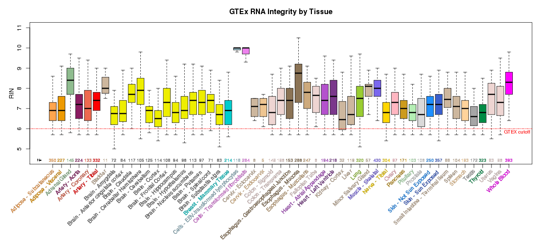
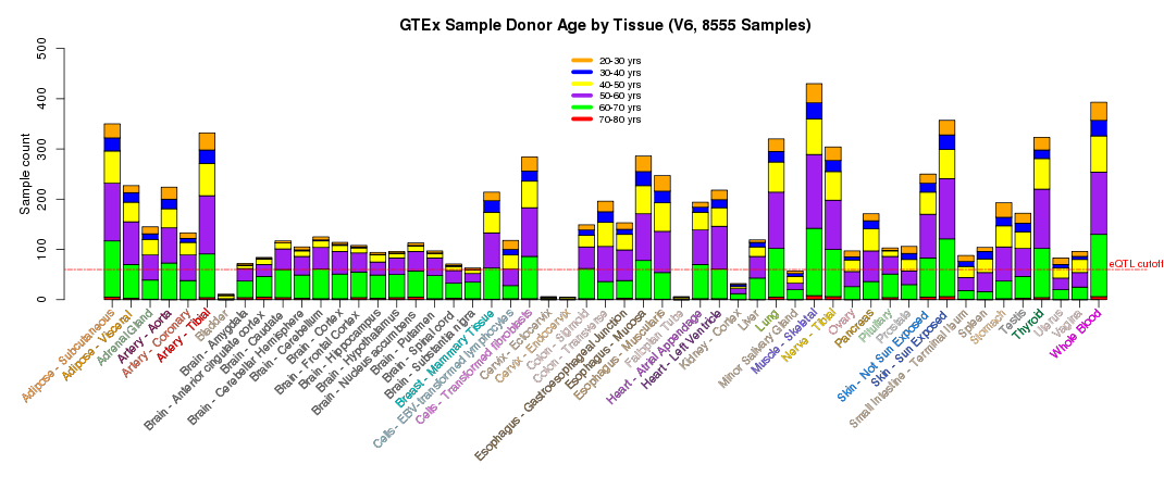
 \
\
 \
MacParland et al. Nat\
Commun. 2018. / CC BY 4.0\
\
\
\
\
MacParland et al. Nat\
Commun. 2018. / CC BY 4.0\
\
\
\
 \
MacParland et al. Nat\
Commun. 2018. / CC BY 4.0
\
MacParland et al. Nat\
Commun. 2018. / CC BY 4.0 \
MacParland et al. Nat\
Commun. 2018. / CC BY 4.0
\
MacParland et al. Nat\
Commun. 2018. / CC BY 4.0 \
\
 \
\
 \
\
